


ABSTRACT
The link between stellar host properties, be it chemical, physical, dynamical, or galactic in nature, with the presence of planetary companions, has been one that has been repeatedly tested in the literature. Several corroborated work has argued that the correlation between a stellar atmosphere’s chemistry and the presence of gas giant companions is primordial in nature, implying that the chemical budget in a protoplanetary disc, and by proxy the eventual stellar host, increases the likelihood of gas giant formation. In this work, we aim to use the power of computer vision to build and test a machine learning classifier capable of discriminating between gas giant host stars and a comparison sample, using spectral data of the host stars in the visible regime. High-resolution spectra are used to preserve any inherent information which may contribute to the classification, and are fed into a stacked ensemble design incorporating several convolutional neural networks. The spectral range is binned such that each is assigned to a first-level voter, with the meta-learner aggregating their votes into a final classification. We contextualize and elaborate on the model design and results presented in a prior proceedings publication, and present an amended architecture incorporating semisupervized learning. Both models achieve relatively strong performance metrics and generalize over the holdout sets well, yet still present signs of overfitting.
1 INTRODUCTION
The question of whether there lies a measurable correlation between planet occurrence and host star chemistry has been a pertinent one for the past few decades. It has been a coveted goal for the field to map out the distribution of planet occurrence with all manner of stellar and orbit parameters (e.g. Johnson et al. 2010; Perryman et al. 2014). How such an occurrence rate is affected by a system’s dynamical history (e.g. Dai et al. 2021), any stellar companion (e.g. Hirsch et al. 2021), or selection effects due to detection techniques (e.g. Clanton & Gaudi 2014, 2016) have also been considered. In any case, efforts to achieve this for all planetary classes, particularly those in the lower mass regime, so far remain inconclusive. Yet, for Jupiter-class exoplanets, there has been several corroborated work reinforcing the hypothesis that certain stellar properties of a planetary-host star yield a higher probability for gas-giant formation in its primordial protoplanetary disc (e.g. Johansen, Youdin & Mac Low 2009; Bai & Stone 2010; Ercolano & Clarke 2010; Schlaufman & Laughlin 2011; Johnson & Li 2012; Buchhave et al. 2014).
As outlined in Perryman (2018), notable work has been done using samples of stars with and without planets, in order to evaluate whether or not there lies an intrinsic, statistically significant difference in chemical abundances and stellar parameters between the two classes (e.g. Buchhave & Latham 2015; Jofré et al. 2015; Maldonado & Villaver 2016; Mishenina et al. 2016; Mulders et al. 2016). Additionally, comparative analysis like that of Thiabaud et al. (2015) aims to discern a consistency between elemental ratios between planets and their respective host stars. What has been made clear through decades of stellar abundance ratio measurements is that the reliability of said ratios relies on the quality of the spectra they are acquired from. High signal-to-noise (SNR) ratios as well as high resolving power are vital for accurate ratios, especially for lighter elements like Li, C, N, O, Na, Al, Mg, and S in solar-type stars, as their number of spectral lines is limited (Gonzalez 2006a; Perryman 2018).
The strongest correlation between planet occurrence and host-star chemistry lies in the corroborated conclusion that metallicity [Fe/H] is intrinsically linked with planet formation (Petigura et al. 2018). Early studies (e.g. Gonzalez 1997; Gonzalez & Laws 2000; Reid 2002) indicated that exoplanet host stars in the solar neighbourhood tend to be metal-rich. However, as it has remained a challenge to reliably measure and reproduce metallicities values, there has been a need for larger and more secure spectroscopic samples of hosts and comparison stars (Perryman 2018). Notable spectroscopic survey work of this type includes: Santos, Israelian & Mayor (2001), Santos et al. (2005), Takeda & Honda (2005), Valenti & Fischer (2005), Bond et al. (2006, 2008), Luck & Heiter (2006), Sousa et al. (2008), Ghezzi et al. (2010), Brugamyer et al. (2011), and Adibekyan et al. (2012b). Considerations have been posed on the origin of the metallicity correlation (as well as any proposed dependencies), and whether or not it is due to the relatively simplistic definition of the parameter itself. To name an example, work done by Haywood (2008, 2009) suggested Galactic location and thin/thick disc location as possible contributors to planet occurrence. In response, Gonzalez (2009, 2014) replaced metallicity in the analysis with a refractory index [Ref/H], to include refractory elements vital for planetary formation (Mg, Si, and Fe). This eliminated the dependencies found by Haywood. Several other sources of bias have been suggested. Paulson & Yelda (2006) discuss certain selection effects in radial velocity surveys (see also Gonzalez 2003, 2006a; Sozzetti 2004), while Fischer & Valenti (2005) argue the impact of the differences in surveys being magnitude-limited and volume-limited. Gonzalez (2014), to attempt to tackle these biases, suggested three corrections that should be applied to the observed relative incidence: ‘diffusion in the stellar atmosphere, use of the [Ref] index in place of [Fe/H] for metallicity, and correction for local sampling with the W-velocity’. Interestingly, with these three corrections applied, an enhanced dependency on metallicity was detected (Perryman 2018). Regardless, comparative analysis on host and non-host stars indicates that the giant planet occurrence rates rise as a function of metallicity (Santos et al. 2005). According to Fischer & Valenti’s (2005) results, at −0.5 < [Fe/H] < 0.0, less than 3 per cent of the stars had Doppler-detected giant planetary companions. For [Fe/H] > 0.3 dex, however, the occurrence rate stood at 25 per cent. Over 0.2–1.9 M⊙, Johnson et al. (2010) observed a weaker dependency, but agreed that giant companions are less likely to orbit around stars with sub-solar metallicity. Gonzalez (2014) detected a stronger dependency than both. Johnson et al. also concluded that at solar metallicity, occurrence rises with M⋆. However, Santos et al. (2017) showed that in the case of giant planets with mass >4MJ, their stellar hosts tend to be more massive and metal-poor, yet for smaller planets, the usual correlation seemed to take hold. In accordance with Santos et al.’s (2017) first point, however, the correlation seems to break down in the case of giant stars, M-dwarfs, stars with intermediate metallicity and the occurrence of lower mass planetary companions (Maldonado, Villaver & Eiroa 2013; Mann et al. 2013; Perryman 2018). In the case of Neptune-mass companions, Sousa et al. (2008) found no rise in occurrence around metal-rich stars. The strongest correlations thus remain in the Jovian planet regime. With regards to M-dwarfs, the drop in giant planet occurrence is plausibly likelier to be due to the star being on the lower end of the stellar mass spectrum. It should be noted, however, that Johnson & Apps (2009) deduced that M-dwarf host stars seem to be systematically metal-rich, with a sample average metallicity of [Fe/H] = +0.16, as opposed to FGK dwarfs with [Fe/H] = +0.15.
Two hypotheses have been proposed to detail the origin of such a difference in metallicity, if it is truly intrinsic. The first is that it is primordial in origin and that metallicity facilitates planetary formation. The second is self-enrichment, due to the accretion of metal-rich material. Whilst both are possible, the first seems far more likely to explain the frequency of the correlation (Perryman 2018). Modelling work based on the core accretion model (Ida & Lin 2004, 2005; Kornet et al. 2005; Wyatt, Clarke & Greaves 2007) successfully showed a dependence of Jovian occurrence on metallicity. Ida and Lin’s model in particular also demonstrates the innate rarity of close-in giant planetary companions around M-dwarfs.
Besides the investigated dependence on the metallicity and refractory indices, relative abundances of specific refractory and volatile elements have been studied, in hopes of exploring whether there lies a discrepancy (Perryman 2018). Thus far, there has been less than convincing evidence of such. While there have been samples in which certain elements have slightly changing abundances in the case of refractory and moderately refractory elements, none have shown a significant or notable trend to lead to talk of a present correlation (e.g. Gonzalez et al. 2001; Takeda et al. 2001; Bodaghee et al. 2003; Beirao et al. 2005; Gilli et al. 2006). As explained in Perryman (2018), the general assertion is that relative abundances of refractory elements in host stars are no different than from other Population I stars. For volatile elements, the results have been similar (e.g. Gonzalez 2006b; Da Silva, Milone & Reddy 2011). r- and s-process elements have also been considered (e.g. Huang et al. 2005; Gonzalez & Laws 2007; Bond et al. 2008), with results from Bond et al. showing a difference in host star abundance as opposed to comparison star and even solar abundances. Therefore, it seems likely that stars tend to be richer in metal mostly due to primordial factors, implying that stars formed in more metal-rich molecular clouds have more favourable odds for planet formation.
In the metal-poor regime, other elements have been presented to aid planetary formation. A number of surveys and results seem to indicate that metal-poor host stars are likely to have an abundance of α-elements (e.g. Haywood 2008, 2009; Adibekyan et al. 2012a, c). Conclusions that were reached are that for low metallicity stars this is evidence that they formed in the Galactic thick disc, and that for metal-poor stars, metals different than Fe might be necessary for planetary formation. Hence, primordial chemistry during stellar formation potentially plays a significant role in aiding planetary formation.
One particular element that may have interesting implications on planetary formation is lithium. Li depletion tends to be present in host stars, that is, compared to similar stars without planetary companions. Several surveys have found low abundances of Li in planet-hosting stars (e.g. Gonzalez, Carlson & Tobin 2010; Delgado Mena et al. 2014, 2015). Israelian et al. (2004) describe a significant difference in Li abundance between hosts and non-hosts with an effective temperature of 5600–5850 K, with any discrepancies dropping off at higher temperatures. If, as Perryman (2018) explains, ‘the presence of planets somehow enhances Li destruction in the star, it raises the possibility of identifying stars likely to host planets solely from a determination of their Li content’. One major issue, however, is that in solar-type stars, only one line Li i (at ∼670.8 nm) is available for spectroscopic detection. However, an isotope that might present direct evidence of planet accretion into a metal-rich solar-type host star is 6Li. As models conclude that it should be destroyed during the pre-main-sequence stage (Forestini 1994), its presence might indicate accretion of planetary material.
For a more complete and in-depth review of the advancements in the field, the reader should be directed towards that in chapter 8 of Perryman (2018), on which this introduction was based.
The challenge in identifying any subtle potential markers in high-quality spectra presents itself as one reminiscent of a data mining problem: vast data sets with dense instances needing to be analysed for any non-trivial patterns. Such patterns are then to be used to classify these instances into distinguishable groups. The advent of machine learning (ML) algorithms and neural networks (NN) in recent years has provided both the tools and the capability to investigate such fine margins hidden within the data.
The application of ML algorithms in classifying stellar spectra is not a novel idea, at least with respect to stellar spectral class. Several endeavours have been attempted in trying to move away from the traditionally manual method of inspecting each spectrum independently to assign a class. As outlined by Sharma et al. (2020), conventional NNs, as well as ML techniques like Principle Component Analysis (PCA), were applied to classify optical spectra in recent decades (e.g. Gulati et al. 1994; Singh, Gulati & Gupta 1998; Manteiga et al. 2009; Gray & Corbally 2014). Furthermore, certain classifiers have been developed which not only consider entire spectra as inputs, but also consider certain specific spectral indices (e.g. Kesseli et al. 2017). While the performance of ‘shallow’ NNs has had promising generalization results, the potential for deeper networks & especially convolutional neural networks (CNNs), for spectral classification, can be even higher. Not unlike their 2D counterparts’ strength in image classification, 1D CNNs do not observe each flux value independently of its neighbouring data points within the spectrum. By design, CNNs are adept in feature extraction through the use of kernels. Such filters comb through the spectral axis in search for class-discriminating features, while ensuring that each flux value is ‘seen’ within the context of the neighbouring values in the sequence (Sharma et al. 2020).
Besides the aforementioned use of NNs, and CNNs in particular, in stellar spectral classification and parameter regression tasks, in recent years the natural sciences have seen a rapid influx of work implementing CNNs to model classification regimes generalized from modestly sized training sets (e.g. Kamilaris & Prenafeta-Boldú 2018; Liu et al. 2019; Naranjo-Torres et al. 2020). Particularly relevant to our work, 1D CNNs have been applied to the spectral classification and spectral feature analysis in bioinformatics, geosciences, molecular analysis, and stellar spectral classification (e.g. DePaoli et al. 2019; Ghosh et al. 2019; Liu et al. 2019; Sharma et al. 2020). What is evident in the majority of previous applications is that the separation between classification labels and classes is clear and definitive, with the assumption that a generalized transformation function is there to be found within the data set. Therefore, as shall be discussed extensively in this paper, for a classifier that is not only attempting to model any potential function separating complex observational data, but additionally mining said data to ascertain if such a function is present, any results obtained need to be conservatively assessed. That being said, the power that CNNs have thus far displayed in spectral classification provides a worthwhile endeavour in the case of Jupiter-hosting stellar spectra.
The growing complexity and availability of powerful classification models and algorithms has been accompanied by a steady development of techniques on how to successfully incorporate several predictive models in one overarching classifier (Rokach 2010). One such ensemble method is stacking, which as proposed by Wolpert (1992), is meant to reduce the generalization error rate of singular classifiers by establishing a second layer of classification. At this layer, an instance’s features are simply each of the singular classifiers’ (henceforth referred to as the first level classifiers) prediction on the original data instance. This allows a potentially strong classifier, aptly termed as a blender or meta-learner, to model each of the individual classifier’s biases on the training data (Wolpert 1992). Thus, provided that the first level classifiers are diverse enough, either in data input and/or architecture, the stacked classifier develops the potential to be a stronger generalizer than any individual model (Seni & Elder 2010).
In this paper, we apply ML techniques to develop a classifier capable of discriminating between Jupiter hosts and comparison stars solely based on the spectral data collected from the planetary system’s host star. The focus was placed on gas giant exoplanets due to the higher overall confidence in the significance of stellar chemistry affecting gas-giant formation. Furthermore, with current technological capabilities, gas giant detection has lower margins of error and higher chances for detection. Thus, any labelling of such a data set of stellar hosts and non-hosts can be done with greater confidence.
It should be mentioned at this point that we present some results from this work in Zammit & Zarb Adami (2023), a refereed proceedings paper of a poster presentation given at the International Conference on Machine Learning for Astrophysics (ML4Astro), held in Catania, Italy in May 2022. The paper describes the labelled data set used here, summarizes the general design employed in our basic model architecture, and briefly goes over the main results of that iteration of the model. This paper builds upon this work by providing a far more extensive description of the data set and model presented in Zammit & Zarb Adami (2023), and continues in describing a second model incorporating unsupervized learning using a second unlabelled data set. We appreciate that this may be redundant, but in doing so, we aim to provide a deeper explanation of the curation and preparation of the data set, as well as describe the basic model architecture in greater detail. The results will be restated and cited from the original proceedings paper to further contextualize their significance within the scope of our work.
We decided to approach the problem through the use of raw high-resolution spectra as direct inputs and to implement a stacked CNN classification architecture to assign a classification probability on whether that spectrum’s star is a Jovian host. A data set was compiled using high-resolution optical spectra observed with either the HARPS (High Accuracy Radial velocity Planet Searcher; Mayor et al. 2003) or FEROS (Fibre-fed Extended Range Optical Spectrograph; Kaufer et al. 1999) spectrographs mounted on the European Southern Observatory (ESO) La Silla 3.6-m telescope and the ESO/MPI 2.2-m telescope, respectively. A particular draw to such a design comes from the fact that if it truly leads to a stable, accurate and precise classifier, such a system could hypothetically serve as a preliminary check for exoplanet detection. The major strength that such a system would provide is that it would aid in narrowing the search space for exoplanet detection, using no extra observation time or instrument dedication, other than the generic form of optical spectroscopy that would already be taking place for stellar parameter acquisition. Furthermore, the spectrum itself would need only be wavelength calibrated and normalized to serve as an input, removing the need for subsequent abundance line fitting and abundance retrieval. Naturally, however, since such a method would not be detecting direct physical evidence of the presence of an orbiting planetary system, it can optimistically only be used as a complementary method to aid in preliminary searches. This work essentially aims to use conventional approaches applied in computer vision in various domains, namely the use of CNN classifiers and autoencoders, to develop a system that facilitates target selection for upcoming surveys and follow-up observations.
As this work is partially motivated by that found in Hinkel et al. (2019) (in which a recommendation algorithm was implemented for Jovian host characterisation), the data set was compiled from entries in the Hypatia Catalogue1 (Hinkel et al. 2014). This catalogue was thus used for a preliminary exploration of the data set prior to training and evaluation.
In Section 2, we discuss our general methodology and structure of the work presented in this paper, outlining how the performance of both networks will be assessed and which major discussion points we will aim to explore. We also conduct some preliminary exploratory data analysis to assess any initial patterns within the data set. In Section 3, we discuss our entire methodology for preparing the data set, as well as a brief overview of the FEROS and HARPS spectra, the Hypatia Catalog and the format in which the observational data was acquired. Once the data set is defined, the following two sections describe the 2 model architectures incorporated for the first-level classifiers. Section 4, we present the model described in the proceedings paper, and cite the training and performance results presented at ML4Astro. Section 5 presents and justifies the overall network architecture, training and performance of the second iteration of the model, in which we incorporate unsupervised learning the train the lower levels of the convolutional base. Finally, we present our concluding discussion points in Section 6, ending with closing remarks and proposals for future work.
2 METHODOLOGY
As was outlined in Section 1, throughout this body of work we aim to utilize the proposed correlation between stellar host (and by extension, planetary disc) chemistry and giant planet formation based on the core accretion model, to design and train a classifier capable of discriminating between comparison stars and likely Jovian hosts. This section will aim to identify the major steps which will be involved, starting with the methodology for obtaining data instances adequate for CNN training, followed by an exploration of said data set to assess any preliminary correlation within the star sample. Since this involves the use of host labels, it should be noted that only the labelled data set is considered in this section. Finally, we discuss preliminary requirements and caveats for the model architecture during training, validation, and testing.
2.1 Data set curation
Defining the problem at hand is crucial during the data set preparation stage, so as to ensure that the data is optimally curated and pre-processed for the model to learn and generalize. As it is a quintessential supervised classification task, each data instance should not only be cleaned from any inherent, unrelated biases but also labelled as confidently as possible. The spectral data set requires that each instance has the same spectral range and resolution, such that each input feature corresponds to the same wavelength across every instance. Furthermore, each spectrum’s natural dependency on temperature will need to be alleviated by normalizing the curve, such that the data instance is set to demonstrate the relative peaks and dips from the spectrum’s continuum. As the number of input features in the spectral data set will be expected to be of the order of 103, the need for a large data set becomes more pressing. Therefore, we allow multiple spectra for each star in the sample, capping the maximum at 25 spectra per star. This choice will be explained further in Section 3.4.
2.2 Data set exploration
Prior to any training and testing, it is fruitful to highlight any preliminary correlations within the data set. To do so, the elemental abundance data of all host and comparison stars in the labelled data set were fetched from the Hypatia catalogue. Fig. 1 plots the frequency of abundance measurements of every element of every star in the sample, with the contribution from the Jovian hosts (23 per cent of the global sample) and comparison stars (77 per cent of the global sample) subsets highlighted to show its variance across the abundance features. If the number of elemental features is restricted to those linked by previous work to correlations with gas-giant formation in accordance with the core accretion model (see e.g. Israelian et al. 2004; Bond et al. 2008; Gonzalez 2008, 2014; Adibekyan et al. 2012b, c; Hinkel et al. 2019), the data set can be reduced to 26 features: Fe, Li, C, O, Na, Mg, Al, Si, Si ii, Ca, Ca ii, Sc, Sc ii, Ti, Ti ii, V, V ii, Cr, Cr ii, Mn, Co, Ni, Y, Y ii, Zr, and Zr ii. The variation in the contribution from Jovian hosts to the available number of abundance measurements can be represented by a whisker plot as shown in Fig. 2. The 4 outlier elements, namely Li, Ca ii, Si ii, and VII, were subsequently omitted from the final data set to avoid data frequency biases.
![Number of stars in the sample with abundance measurements (in [X/H]) for every listed element. Each set has been separated into Jovian hosts and comparison stars, with the global sample consisting of a 23/77 split between the two subsets.](https://oup.silverchair-cdn.com/oup/backfile/Content_public/Journal/mnras/527/4/10.1093_mnras_stad3668/1/m_stad3668fig1.jpeg?Expires=1750276831&Signature=EJdnWBE6vRkFizRGa8Wu4bG3Xxq798UermR~kRKG5u~ZbPytBqYK4heQ3m0rOvIqaiGcL7L6PCsfEp8EdzYIyKItRFSYuiYI8w0fkK~IKQZjNyvH4F-kd9atBk~asbeecPIgInodwT3eNBniRX6XIatNJISnOapTkSa-ki7tFT5x1yA2s0vHHfT9OzJSj-SBWwN7ex3vUzqxV-MKLZNEnsD52~3CKeXdbCuUqNz-bStUrT3~mDv~ZizGByLjFOUftVr2KitpOXTmyX-Eo5IfGuWgm6Lxnpyz8RYVz~~OeNe7k9n9on4RQKuiKBmnrK0C2NM7gzE73Q4kvZymkwhv6g__&Key-Pair-Id=APKAIE5G5CRDK6RD3PGA)
Number of stars in the sample with abundance measurements (in [X/H]) for every listed element. Each set has been separated into Jovian hosts and comparison stars, with the global sample consisting of a 23/77 split between the two subsets.
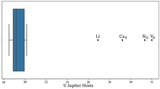
A whisker plot showing the distribution of the percentage of abundance measurements which belong to Jovian hosts. The outlier elements, namely Li, Ca ii, Si ii, and V ii, are labelled and subsequently omitted from the feature list.
With the abundance features selected, each element’s distributional statistics across the stellar sample can be addressed. In Fig. 3, the Jovian hosts tend to display greater abundance measurements for all 22 elements in our sample, and a two-sample Kolmogorov–Smirnov test shown in Table 1 suggests that the correlations between their presence in stellar atmospheres and gas giant occurrence suggested in previous work should be expected to be present in the data set. Hence, with an early indication that the Jupiter hosts in the sample are chemically distinct from the comparison star subset, the data set explored in this paper has early potential to allow us to approximate a transformation function capable of discriminating between the two classes.
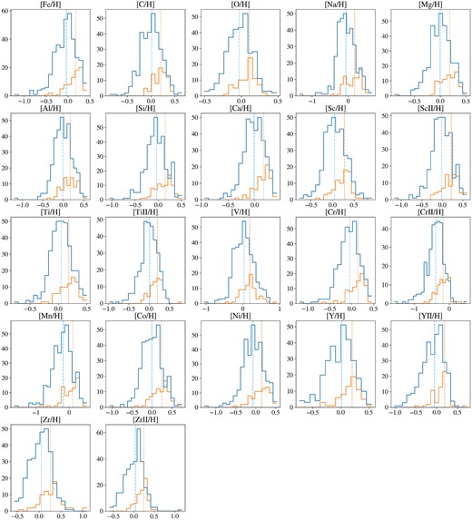
Distribution of abundance measurements in the stellar sample for each of the selected 22 elements. A two-sample Kolmogorov–Smirnov test was done to check the likelihood that both subsets belong to the same parent population, and the p-values are given in Table 1. All elements tend to show greater abundances in Jupiter hosts relative to the comparison stars in the sample, suggesting an intrinsic chemical disparity between the two classes.
A two-sample Kolmogorov–Smirnov test was done for every relative abundance in Fig. 3 to check the likelihood that both subsets belong to the same parent population. The p-values are listed here.
| Rel. abundance | p-value | Rel. abundance | p-value | Rel. abundance | p-value |
|---|---|---|---|---|---|
| Fe/H | 9.9 × 10⁻¹⁰ | C/H | 4.5 × 10⁻⁹ | O/H | 4.6 × 10⁻⁴ |
| Na/H | 5.4 × 10⁻⁷ | Mg/H | 1.4 × 10⁻⁷ | Al/H | 1.1 × 10⁻⁵ |
| Si/H | 1.9 × 10⁻⁷ | Ca/H | 3.9 × 10⁻⁹ | Sc/H | 2.1 × 10⁻⁷ |
| ScII/H | 3.3 × 10⁻⁹ | Ti/H | 9.9 × 10⁻⁷ | TiII/H | 5.8 × 10⁻¹⁰ |
| V/H | 5.8 × 10⁻⁵ | Cr/H | 1.8 × 10⁻⁸ | CrII/H | 3.9 × 10⁻⁹ |
| Mn/H | 4.8 × 10⁻⁹ | Co/H | 6.1 × 10⁻⁹ | Ni/H | 1.4 × 10⁻⁷ |
| Y/H | 4.6 × 10⁻⁶ | YII/H | 1.1 × 10⁻¹⁰ | Zr/H | 7.7 × 10⁻⁷ |
| ZrII/H | 2.5 × 10⁻⁸ |
Shifting our focus to the raw spectra in particular, it is of stressed importance (as stated in Gonzalez (2006a) & Perryman (2018)) for stellar abundance measurement retrieval that the SNR of the spectrum is high enough to allow for accurate estimation of the equivalent widths of specific spectral lines. This is especially true for several lighter elements (particularly Fe, Li, C, O, Na, and Mg) which have been shown to correlate with giant planet formation, as their number of spectral lines is limited.
An initial concern when selecting the instances to include in the data set was that the need to collate a large enough data set for training, mitigated by the use of CNNs and a stacked architecture, would naturally lead to the inclusion of observations with moderately lower SNR. It could be argued that the inclusion of the lower percentile SNR spectra could diversify the data set, leading to a certain invariability to SNR values during inference post-learning and generalization. However, it is vital that the instances are clean enough for the model to be able to discriminate between the two classes. We chose to use down to the 50th percentile of possible instances and cap the maximum number of observations to 25 for each target star, resulting in the SNR distribution of the selected instances shown in Fig. 4. The distribution shows a median SNR value of 165.6 and a positive skewness towards higher-SNR observations. With SNR = 100 being equal to the 12.25th percentile, it was deemed acceptable in favour of an adequately large data set and a relatively diverse set of host and comparison stars.
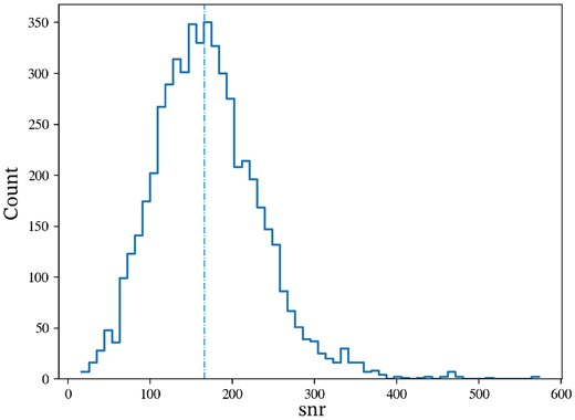
Observational SNR distribution for all instances in the labelled data set. With a median SNR of 165.6 and 87.75 per cent of the instances having an SNR greater than 100, it was a preliminary conclusion prior to training and testing that the extent of the trade-off between SNR variance and data set size was acceptable.
2.3 Model design, hyperparameter selection, and evaluation
After initial exploratory analysis, the selection of model design and methodology in training and evaluating performance could begin. In this section, we aim to explain our reasoning when selecting the general model architecture, the types of ML algorithms implemented and the performance measures used to assess the strength of both classifiers.
Using raw, high-resolution spectra as inputs into a neural network will immediately invoke the curse of dimensionality, even more so in the case when the data set size is not of the order of >105. Hence the model architecture needed to mitigate that to a degree and allow for stable learning and generalization. Hence, we spectrally bin each data instance and employ a stacked ensemble classifier, composed of individual CNN classifiers each responsible for assigning a class based solely on their respective spectral bin. Each of these first-level classifiers feeds a probability score to the upper-level meta-learner, which then aggregates the scores and assigns a final classification. This would further allow us to include a certain level of localization in the system. Observing which spectral bins lead to greater learning and generalization leads to the natural supposition of the location of any potential planetary markers hidden within the spectra.
Focusing on the problem of spectral classification conceptually, it can be treated similarly to image classification and viewed in terms of computer vision, for which CNNs have in particular shown to be quite adept at handling. Furthermore, CNNs tend to show strengths in their ability to identify the presence/absence of a marker within the context of the whole data instance. This led to the decision that a 1D-CNN-based architecture, provided that its depth is not unrealistic to learn and generalize over our data set, would be the optimal choice as the archetype first-level classifier.
In practice, the logistics of training a stacked generalizer is simple. A training set is split in two: one generic training set used to train each of the individual first-level classifiers, and a hold-out set, which is used to train the meta-learner (or blender). Once the first-level classifiers are trained, they are each individually fed the hold-out set to produce inferred predictions. Said predictions are then used as a training set for the blender (Rokach 2010).
To train the individual first-level classifiers, we employ two methods. The first was to simply use the first training subset of the labelled data set to train the entirety of the CNN architecture, as would traditionally be done in a typical ML classification problem. The second method was to incorporate a second, much larger unlabelled data set to train a convolutional autoencoder. The trained encoder network would then serve as the convolutional base of the CNN classifier, such that the labelled data set would then be used to train the dense network placed on top of the encoder. If necessary, deeper levels of the convolutional base can also be trained at this stage. Whilst this will be explained in more detail in Section 5, it would be fruitful to discuss the benefits and drawbacks of each technique. A simple campaign of total supervised learning requires far less computational load and data set curation. It also provides a baseline for the potential strength of generalization which can be expected from the classifier. Incorporating unsupervised learning in the form of an autoencoder does, however, allow the convolutional base to learn a stronger encoding representation from a far larger data set, without the need to label all instances. Allowing the optimizer to focus on only tuning the classifier block (and potentially a small number of deeper-level convolutional layers) when the training is supervised should be expected to lead to steadier and/or stronger performances, provided that the encoding representation learnt from the unlabelled data set optimally compresses the spectrum without losing too much pertinent information.
3 DATA SET PREPARATION
The heart of an ML task, as important as the choice of architecture and the training regime employed, is the data set curation, design, and preparation. This section will explain our methodology in preparing the training, validation, and test sets, both labelled and unlabelled, for training all architectures presented in this work.
A primary requirement for supervised learning is a large data set of labelled instances, so as to train, validate, and test the model and ensure that the transformation function’s weights reliably provide a generalisable fit. Particularly in the case of the CNN architecture, the need for a sizeable data set is a pressing one, as it avoids risks of the transformation function overfitting the training set and limiting generalization (Sharma et al. 2020). In order to make sure the data set is as clean and confidently labelled as possible, several selection rules were observed within our methodology in both collecting spectra and setting labels for each respective instance. This data set is described and originally presented in Zammit & Zarb Adami (2023), but as it is instrumental to the results presented here and the choice of network architectures described in Sections 4 and 5, a full description of the selection and pre-processing methodologies will be given here for context.
Whilst simpler in terms of curation, it is nevertheless crucial for unlabelled data sets to be clean and methodically prepared, following a strict methodology similar to that imposed on to the labelled data set bar the step of labelling the instance. Naturally, each instance has to be of the same form, with the same number of input features, implying that in the case of 1D-spectra, the spectral resolution, and flux representation have to be systematically equal.
Wherever necessary, the explanation will incorporate any deviations in methodology between the preparation of the labelled and unlabelled data sets. Otherwise, the step mentioned can be assumed to be identical for both. As will be explained in Section 3.4, the spectral data set was comprised of HARPS and FEROS spectra obtained through the ESO Science Archive Facility.2 The list of ESO programmes from which the data was taken can be found in the acknowledgements. All stars within the labelled sample have entries in the Hypatia catalogue, in order to allow for the exploratory analysis presented in Section 2.2.
3.1 ESO-HARPS spectra
The HARPS3 (Mayor et al. 2003) has been a significant contributor to radial velocity surveys since it saw first light in 2003. The ESO facility is fibre-fed by the Cassegrain focus of the 3.6-m telescope at the La Silla observatory. By design, HARPS is an échelle spectrograph capable of operating in two modes, a high accuracy mode (HAM) with R = 115 000, and a high-efficiency mode ‘EGGS’ with R = 80 000 (Poretti et al. 2013). As detailed in Perryman (2018), a spectral range of 0.378–0.691μm is covered by the N = 89–161 échelle orders. Thermal spectral drift, as well as that which would be caused by air pressure fluctuations, is eliminated with the vacuum vessel in which the spectrograph is placed. A Th–Ar or background sky reference spectrum is fed into the system in a separate fibre to that through which the target starlight spectrum is fed (Rupprecht et al. 2004). The resultant stability allows for long-term radial velocity accuracy of the order of 1 m s−3.
3.2 ESO-FEROS spectra
The FEROS4 (Kaufer et al. 1999) is a prism-cross-dispersed échelle spectrograph mounted to the MPG/ESO-2.2-m telescope at La Silla. Thermally controlled and bench-mounted, FEROS is capable of an R = 48 000 resolution with a high 20 per cent efficiency, allowing for radial velocity accuracies of ∼25 m s−1 or better. While this implies that it is not as well-suited for radial velocity work and high-resolution spectroscopy as HARPS, FEROS’ considerable spectral range from ∼350 to ∼920 nm over 39 échelle orders provides great potential for spectral analysis.
3.3 The Hypatia catalogue
The Hypatia catalogue1, curated and published by Hinkel et al. (2014), is an unbiased data set of spectroscopic abundance data from 233 different literature sources for a total of 9982 stars in the solar neighbourhood and 80 elements and species. The catalogue also includes stellar properties, and specifically lists which stars are exoplanet hosts. In their exploration of the initial iteration of the catalogue upon publication, Hinkel et al. (2014) determine that for stars within the solar neighbourhood, there could lay an asymmetric elemental abundance distribution, such that ‘a [Fe/H]-rich group near the mid-plane is deficient in Mg, Si, S, Ca, Sc ii, Cr II, and Ni as compared to stars farther from the plane.’
3.4 Data set selection
A strict methodology was put in place while selecting spectra, to ensure that the data set is clean and absent of any major sources that hinder the classifier’s accuracy and ability to generalize. However, as it was naturally vital to generate a large enough data set to train, validate, and test the model such that it could be confidently assessed, our selection rules had to be lenient without damaging the reliability of the data set. Since different observation settings and conditions inevitably cause each imaging campaign to produce slightly different spectra for each observation, a maximum of 25 spectra of each target star which satisfy our selection rules were considered as separate instances in our data set. As this work is partly focused on generalizing a model capable of detecting Jupiters from spectroscopic observations, the use of several spectra of one source can be deemed acceptable in favour of collating a trainable data set.
Since the number of star samples was limited, to accumulate substantially sized training and holdout sets the star sample present in each subset of the data is not disjoint from the rest. This inherently means that at some level there is information bleeding across the data sets, which needs to be kept in consideration when assessing the results. It should also be acknowledged, however, that each spectra within the observational sample of one star will be unique in its level of noise (and by extension its SNR value). This, added to the fact that out the maximum 25 spectra, not all are necessarily from the same facility, would introduce a level of sample diversity which would differentiate between spectral observations of the same star. If the classifier performs well and is stable in its overall generalization, and since the number of maximum spectra per star is more than two orders of magnitude smaller than the data set size (three orders for the pre-trained model), then it would still indicate that the model is inherently decoding the spectral information and learning to differentiate between the two classes. For this iteration of the data set, if we separate by star sample in the training and holdout set, such that no star is an instance in both, the number of target stars in the test set would be significantly limited. This is expected to introduce stellar astrophysical biases which will mask any inherent behaviour that our performance metrics aim to analyse. While it would alleviate the problem regarding the bleeding of information, dividing the data set this way will risk overestimating or underestimating the generalization over the test set, without it being necessarily clear which is occurring. Hence the choice of an instance-independent stratified sampling strategy was deemed to be less susceptible to stellar biases, and the data set was only stratified based on label and facility. We appreciate that this is a major caveat in our work and results; however, the data curation at this stage requires this compromise in favour of accumulating a data set of a substantial size.
3.4.1 Labelled data set
During our first phase of selection for the labelled data set, a query was created to filter all FEROS and HARPS spectra available on the ESO Data Archive2 for target stars which are listed on the Hypatia catalogue. A cross-reference between our spectral data set and the abundance values of all targets within the sample ensured that any inherent biases within the star sample are accounted for. The resultant query was filtered such that each target star was capped to 25 spectra, selecting those with an SNR within the highest 50th percentile for that particular target star.
Once the selection process was completed, a data set of 5417 instances of 434 stars was compiled and ready to be prepared for use. The modest size of the first-layer training set meant that limitations had to be placed on the architecture of the individual CNNs, an issue which will be further discussed in Section 4.1. Spectra were fetched and downloaded from the ESO servers as wavelength-calibrated 2D-spectra stored in Flexible Image Transport System (FITS) files.5
3.4.2 Unlabelled data set
The selection process for the unlabelled data set was by design less strict. The principle aim of the unsupervised training on this data set was for the model to learn how to use a spectral input and encode a compressed representation which optimally preserves as much information from the original spectrum. Therefore, we compiled a data set of FEROS and HARPS spectra from the ESO Data Archive, applying a similar rule to the data set in that the maximum number of spectra per target was set to 25, selecting only those spectra with an SNR within the highest 50th percentile. Targets were selected on the basis that they are not present within the labelled sample, to ensure that at the supervised learning stage, the training, and more importantly validation and testing, would not be biased and unreliable.
A final unlabelled data set of 25 168 instances of 3343 stars was curated, allowing us the freedom of exploring relatively deep convolutional autoencoder architectures without the pressing worry of not having a large enough training set5.
3.5 Training labels
As vital as in the data selection process, it was made sure that labels to the training data are confidently assigned. As the class distinction selection for this work is whether or not the host star in question has a Jovian-class companion, it was important that prior observations and analysis were taken into account. Planetary class designations in the ExoKyoto6 database and NASA Exoplanet Archive7 were taken into account so as to conservatively assign classes to well-studied exoplanets harboured by stars which already passed our set of selection rules. It should be noted of course that it is perfectly possible for any of these stars to have Jovian planets that are yet undetected and, by extension, unaccounted for in our labelling. We discuss the implications this poses in Section 6.
3.6 Pre-processing
The final step in preparing the data set for training was to normalize the data and process it into a model-readable format. Starting off with every instance comprised of the data format as mentioned in Section 3.4, the first important step was to ensure that the spectra are calibrated such that the spectral range and resolution of each bin is invariant to the facility used to collect them. Thus, both FEROS and HARPS spectra were truncated and spectrally binned such that all spectra comprised 104 350 datapoints across the same spectral range (∼3781–6912 Å). Using the specutils8python library, we then generate a fit for the spectrum’s continuum to then use for normalization by
as shown in Fig. 5. Once the flux was normalized, the spectrum was binned into 25 spectral ranges of 4174 datapoints each.
The number of bins was selected through a back-of-the-envelope calculation upon reviewing the plot shown in Fig. 6, in which the number of datapoints allocated to each spectral bin is plotted against the selected number of bins. The dashed horizontal line represents the minimum number of data samples to which both model designs will be exposed to prior to final testing on the test set. It was judged to be a substantial pre-requisite to ensure that the number of input features falls below this value, whilst also keeping practicality and computational load (in terms of the training schedule) in mind. A bin number of 25 was selected arbitrarily, rather than say 24 or 26. Within the immediate range below the threshold, it is not expected that model performance will be significantly sensitive to small changes in the number of bins, mainly due to the relatively high resolution of the spectra.
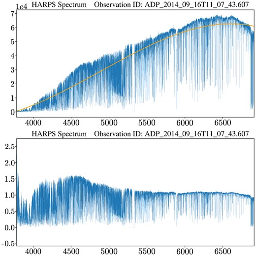
The spectrum, in this case of observation ID ADP 2014:09:16T11:07:43.607, is normalized relative to its continuum, obtained using the specutils library. The upper plot shows the original wavelength-calibrated raw spectrum in blue and the spectrum continuum in orange. The lower plot shows the resultant normalised spectrum ready to be spectrally binned.
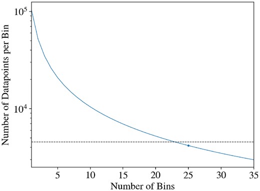
The number of datapoints allocated to each spectral bin against the selected number of bins, with the chosen configuration marked on the solid curve. The dashed horizontal line represents the total minimum number of data samples to which both model designs will be exposed prior to final testing on the test set. The selected number of bins was chosen such that it falls below this value, whilst also considering the trade-off with practicality and computational load.
With the procedure done for every instance, each data set bin was ready to serve as an input for its respective CNN classifier.
3.6.1 Labelled data set
We implement a stratified shuffle split to first divide our data set into a training and test set using a 75/25 split, then again to divide the training set into two subsets with a 75/25 split, the larger of which was used to train the first-level classifier, and second training set for training the meta-learner. The test set was also split in two using a 65/35 split, with the smaller subset being used throughout the training process as a validation set to ensure our hyperparameters maximise learning and generalization without the risk of severe overfitting. The stratification was done by training label and by facility to ensure each data set has the same proportion of HARPS and FEROS spectra, as well as the same ratio of hosts to comparisons. Table 2 shows the resultant sizes of all 4 data subsets.
The number of instances within both training sets for the first-level classifiers and meta-learner used for supervised learning, and the validation and testing sets used to check for maximised and stable generalization.
| Labelled data set | Number of instances |
|---|---|
| 1st level training set | 3046 |
| Meta-learner training set | 1016 |
| Validation set | 475 |
| Test set | 880 |
| Labelled data set | Number of instances |
|---|---|
| 1st level training set | 3046 |
| Meta-learner training set | 1016 |
| Validation set | 475 |
| Test set | 880 |
3.6.2 Unlabelled data set
As the purpose of the convolutional autoencoder was to train the encoding layers for subsequent supervised learning of the final classification architecture, the unlabelled data set was solely split into a training set and validation set. A 90/10 stratified shuffled split was used, stratified solely by the facility from which the instance was observed. The resultant size of the two subsets is shown in Table 3.
The number of instances within the training and validation set of the unlabelled data set, to be used to train the convolutional autoencoder.
| Unlabelled data set | Number of instances |
|---|---|
| Training set | 22651 |
| Validation set | 2517 |
| Unlabelled data set | Number of instances |
|---|---|
| Training set | 22651 |
| Validation set | 2517 |
4 BASIC MODEL: DESIGN AND RESULTS
With the data processed and prepared for training, the basic classifier model was selected and implemented. This section aims to describe the network architecture and algorithms, the ways in which their performance during training was assessed, and the final training plots and performance metrics of both the first-level classifiers and the meta-learner.
As described in Section 2.3, the general architecture follows a stacked ensemble design, with the first level classifiers each designated a spectral bin, as shown in Fig. 7. These voters then output a probability score on whether the spectrum belongs to a Jupiter host, which will collectively be fed as input features to the meta-learner to aggregate to a final classification.
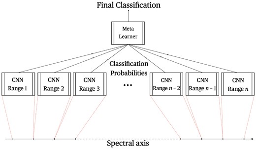
General network architecture of the stacked CNN spectral classifier. Each spectral bin is fed to the respective first-level CNN classifier, which in turn then assigns a classification probability score to be used as an input feature by the meta-learner. The meta-learner then aggregates these probability scores (from all first-level classifiers which demonstrate any form of generalization) to predict a final classification for the data instance.
4.1 System architecture
The aim at this stage of the project is to use a simple architecture which has a certain level of malleability, in the sense that its hyperparameters would allow for the model to be versatile enough for it to adequately suit the classification of each spectral bin during the cross-validation hyperparameter tuning stage of training.
4.1.1 First-level classifier design
The implemented model design follows the structure of an input layer, followed by 2 packs of 1D-convolutional layers separated by a maximum pooling layer. A second pooling layer is placed after the second pack, the output of which is flattened and fed into a fully dense network. The neurons in the dense layers monotonically decrease to a single neuron layer with a sigmoid activation function to output a classification score.
The architecture, as shown in Fig. 8, is designed to have 8 hyperparameters in total, each describing a particular design or functional component of the architecture. The convolutional network component of the model is defined by 5 hyperparameters: n_conv1d_packs describes the number of convolutional layers incorporated into each of the 2 aforementioned packs. Each convolutional layer implements a relu activation function and the kernel size is determined by the hyperparameter kernel. The number of filters for each pack is defined by n_filters_pack1 & n_filters_pack2 respectively. The pooling size of both maxpool layers is then defined by maxpool. Finally, the dense network component is defined by two hyperparameters. n_dense_hl sets the number of dense hidden layers incorporated into the classifier, with each layer again using relu activation function. n_neurons_first sets the number of neurons of the first hidden layer. The subsequent layers then progressively half the number of neurons, ultimately converging to the single neuron dense layer with sigmoid activation function.
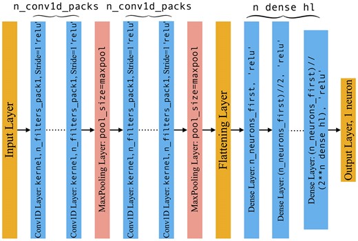
Model architecture for the spectral first-level CNN classifiers.
Batch normalization layers are implemented throughout the architecture, and to introduce model regularisation and avoid overfitting, dropout layers are also included in between the convolutional packs before pooling. The final hyperparameter dropout defines the dropout rate of this layer. The model is finally compiled, implementing a binary_crossentropy loss function defined as
and the Adam optimiser as described in Kingma & Ba (2014), ‘an algorithm for first-order gradient-based optimization of stochastic objective functions, based on adaptive estimates of lower-order moments’. For Adam, we employ the default hyperparameter settings incorporated into the Keras API as suggested by Kingma and Ba and displayed in Table 4 for completeness.
Default hyperparameter values used for the Adam optimizer.
| Hyperparameter | Value |
|---|---|
| lr | 0.001 |
| beta_1 | 0.9 |
| beta_2 | 0.999 |
| epsilon | 1 × 10⁻⁸ |
| decay | 0.0 |
| Hyperparameter | Value |
|---|---|
| lr | 0.001 |
| beta_1 | 0.9 |
| beta_2 | 0.999 |
| epsilon | 1 × 10⁻⁸ |
| decay | 0.0 |
The hyperparameter values for each spectral bin were selected through a randomised 3-fold cross-validation search with the hyperparameter grid as shown in Table 5.
Explored values for all model hyperparameters of the first-level classifiers.
| Hyperparameter | Explored values |
|---|---|
| n_conv1d_packs | 3, 5 |
| n_filters_pack1 | 16, 32, 64, 128 |
| n_filters_pack2 | 16, 32, 64, 128 |
| kernel | 0, 0.1, 0.2, 0.25, 0.35 |
| maxpool | 2, 4, 8 |
| n_dense_hl | 1, 3 |
| n_neurons_first | np.arange(100, 275) |
| dropout | 0, 0.1, 0.2, 0.25, 0.35 |
It is important to stress that at this stage of our work, loss function optimization is not the priority, but rather to test the working hypothesis of an intrinsic chemical discrepancy between the classes and not an instrumental artefact hidden in the data. We discuss the potential for different designs in Section 6. For training, a batch size of 32 and early stopping of 50 epochs were implemented.
4.1.2 Meta-learner design
Once all the first-level classifiers were trained, the next step was to design the meta-learner of the overarching architecture. As it was expected that not all spectral bins should necessarily host class-discriminating features, the number of input features per sample greatly depended on each first-level classifier’s ability to learn and generalize over their spectral region of the labelled data set.
If the number of input features is assumed to be equal to the number of first-level voters,then the required model affords to be relatively shallow with a conventional design. We incorporate a simple neural network architecture, composed of a number of dense layers in between the input layer and a final single-neuron dense layer with a sigmoid activation function to output a final probability score to determine which class the instance is expected to belong to. The dimensions and specifics of the architecture are determined through 4 custom hyperparameters set when building the network: n_dense_hl sets the number of hidden layers in the network, n_neurons_first sets the number of neurons in the first hidden layer, a number which is halved with each progressive layer, activation_fn dictates the type of activation function used for every dense hidden layer, and optimizer_type sets the optimiser implemented during training. We employed 3-fold cross-validation in a random search to explore the hyperparameter space and tune our model. Table 6 presents all the explored values.
Explored values for all model hyperparameters of the meta-learner for the basic model design.
| Hyperparameter | Explored values |
|---|---|
| n_dense_hl | 1, 3, 5 |
| n_neurons_first | np.arange(100, 750) |
| activation_fn | ‘selu’, ‘elu’, ‘relu’, ‘tanh’, ‘softsign’ |
| optimizer_type | ‘adam’, ‘adagrad’, ‘nadam’, ‘sgd’ |
| Hyperparameter | Explored values |
|---|---|
| n_dense_hl | 1, 3, 5 |
| n_neurons_first | np.arange(100, 750) |
| activation_fn | ‘selu’, ‘elu’, ‘relu’, ‘tanh’, ‘softsign’ |
| optimizer_type | ‘adam’, ‘adagrad’, ‘nadam’, ‘sgd’ |
4.1.3 Control test with common classification methods
To comparatively assess the performance seen by the basic model design and validate the choice in a CNN design for the first-level classifiers and ANN design for the meta-learner, we replace all individual classifiers within the stacked architecture with one of two common classification methods. This should provide a baseline on whether the choice of architecture contributes to stronger and more consistent generalization. This method, rather than simply replacing the entire stacked classifier with one single model, maintains the compromise taken in the design to alleviate the impact of the curse of dimensionality whilst allowing for direct testing of the architectures chosen within the ensemble.
The chosen classification methods are a Support Vector Machine (SVM) classifier, which is characteristically well-suited for tasks in which the data set size can be somewhat limited, and a Random Forest (RF) classification model, which provides another ensemble method within the framework. The hyperparameters are tuned using a randomized search cross-validation, as is the case with our model. Since the number of responsive classifiers differs between the basic and autoencoder base models, this is reflected in the selection of first-level voters to be fed into the meta-learner. The performance metrics in each case will be presented in tables alongside our results of both proposed designs, namely Tables 7 and 8.
Comparative performance metrics (for the basic model design) of the meta-learner in the stacked SVM and RF models, set with a labelling threshold of 0.5 and 0.65. Results suggest clear overfitting, and generalization scores are weaker and more erratic than those of our basic model presented in Table 10.
| Data set | Accuracy | Precision | Recall | F1 score | |
|---|---|---|---|---|---|
| Threshold set to 0.5 | |||||
| 1st Level training set (%) | SVM | 97.54 | 98.46 | 90.75 | 94.45 |
| RF | 100.0 | 100.0 | 100.0 | 100.0 | |
| Meta-learner training set (%) | SVM | 89.07 | 79.15 | 71.37 | 75.06 |
| RF | 96.75 | 98.09 | 87.61 | 92.55 | |
| Validation set (%) | SVM | 88.24 | 78.72 | 67.27 | 72.55 |
| RF | 89.71 | 81.44 | 71.82 | 76.33 | |
| Test set (%) | SVM | 88.85 | 81.71 | 66.34 | 73.22 |
| RF | 89.08 | 86.81 | 61.88 | 72.25 | |
| Threshold set to 0.65 | |||||
| 1st level training set (%) | SVM | 97.54 | 98.46 | 90.75 | 94.45 |
| RF | 100.0 | 100.0 | 100.0 | 100.0 | |
| Meta-learner training set (%) | SVM | 89.07 | 79.15 | 71.37 | 75.06 |
| RF | 94.69 | 100.0 | 76.92 | 86.96 | |
| Validation set (%) | SVM | 88.24 | 78.72 | 67.27 | 72.55 |
| RF | 90.34 | 91.03 | 64.55 | 75.53 | |
| Test set (%) | SVM | 88.85 | 81.71 | 66.34 | 73.22 |
| RF | 88.85 | 95.61 | 53.96 | 68.99 | |
Comparative performance metrics (for the autoencoder base model design) of the meta-learner in the stacked SVM and RF models, set with a labelling threshold of 0.5 and 0.45. Results suggest clear overfitting, and generalization scores are weaker and more erratic than those of our autoencoder base model presented in Table 15. For an explanation on how these differ from the metrics in Table 7, refer to Section 4.1.3.
| Data set | Accuracy | Precision | Recall | F1 score | |
|---|---|---|---|---|---|
| Threshold set to 0.5 | |||||
| 1st level training set (%) | SVM | 91.17 | 92.55 | 67.14 | 77.82 |
| RF | 100.0 | 100.0 | 100.0 | 100.0 | |
| Meta-learner training set (%) | SVM | 86.22 | 77.98 | 55.98 | 65.17 |
| RF | 95.28 | 98.44 | 80.77 | 88.73 | |
| Validation set (%) | SVM | 84.03 | 72.97 | 49.09 | 58.70 |
| RF | 89.92 | 85.23 | 68.18 | 75.76 | |
| Test set (%) | SVM | 84.64 | 76.38 | 48.02 | 58.97 |
| RF | 88.85 | 82.91 | 64.85 | 72.78 | |
| Threshold set to 0.4 | |||||
| 1st level training set (%) | SVM | 91.17 | 92.55 | 67.14 | 77.82 |
| RF | 100.0 | 100.0 | 100.0 | 100.0 | |
| Meta-learner training set (%) | SVM | 86.22 | 77.98 | 55.98 | 65.17 |
| RF | 96.36 | 93.39 | 90.60 | 91.97 | |
| Validation set (%) | SVM | 84.03 | 72.97 | 49.09 | 58.70 |
| RF | 88.87 | 78.79 | 70.91 | 74.64 | |
| Test set (%) | SVM | 84.64 | 76.38 | 48.02 | 58.97 |
| RF | 88.85 | 80.23 | 68.32 | 73.80 | |
4.2 Training performance and results
A full assessment of the performance during training should be segregated into two parts. First, the performance of the individual first-level classifiers should be independently assessed, so as to discern which bin ranges show a greater propensity for learning and generalization, whilst simultaneously gauging which hyperparameter settings and regularisation techniques yield the most effective results. Then, the performance of the meta-learner can be judged in the context of the first-level classifier it is fed from. At this point, the final classification results and performance on the test set can be assessed.
4.2.1 Performance of first level classifiers
As we stress in Zammit & Zarb Adami (2023), the first-level classifiers in the basic model significantly overfit the first training set, with several showing no clear signs of generalization. Three ranges however show clear minimization of the validation loss, albeit whilst still overfitting, as shown in Figs 9 and 10.
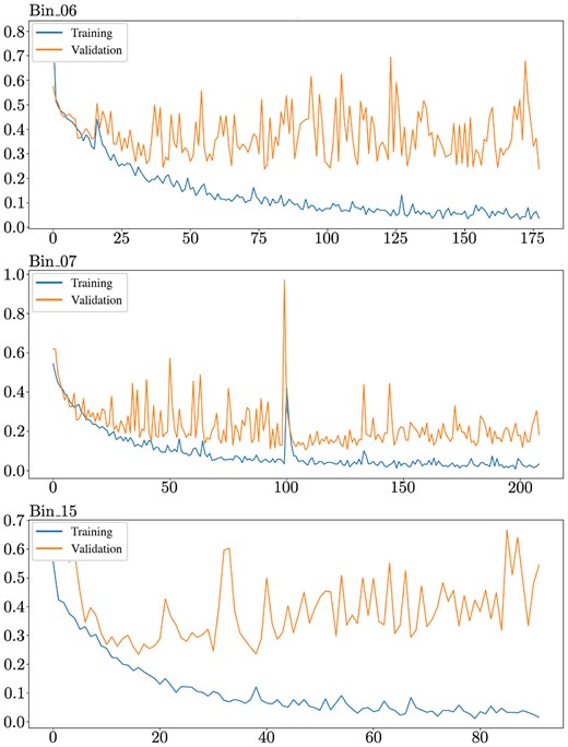
The training and validation loss of the 3 responsive first-level classifiers.
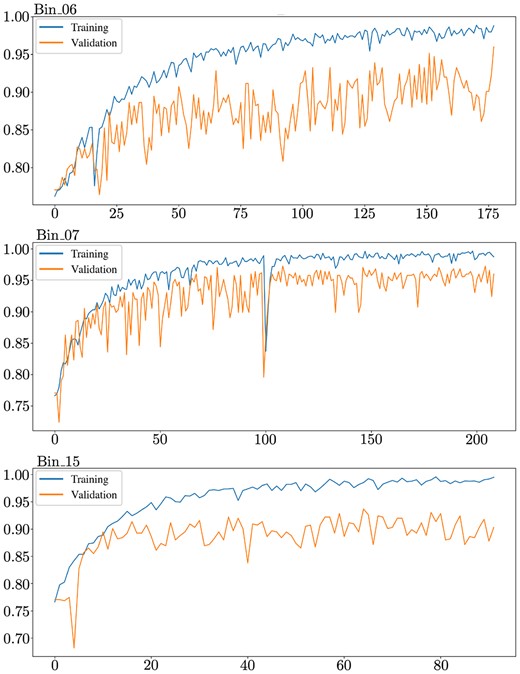
The training and validation accuracy of the 3 responsive first-level classifiers.
As is clear in the performance on all three bins, the validation curves are all far more erratic than their training curve counterparts, suggesting that while generalization is still occurring, even if to a minimal extent, it is clearly not stable enough and warrants further modifications. This reinforces the suggestion that the generalization of the models is unstable and that the optimal transformation function has not been approached. Prior to any meta-learner training, this can imply some preliminary implications on what should be expected. As we state in Zammit & Zarb Adami (2023), this lack of a stable convergence should be expected to manifest itself in reduced performance on the second training set. The output predictions from these first-level classifiers are fed as input features to the meta-learner, and should thus affect the latter’s ability to approximate its ideal transformation function if their generalization is currently not fully reliable.
This all being said, it should still be acknowledged at this stage that at least in these three bins, there is some form of convergence with the basic model. This suggests that with a large enough data set or properly tuned model, convergences could be expected to be more stable and consistent, at the very least for these three bins, and potentially for the other bins as well. Table 9 describes the responsive bins, including their respective spectral range and the performance of their best-performing model on the training and validation sets. The model weight magnitudes assigned by the meta-learner in the first layer to the features corresponding to these three bins are also listed, along with the ranking of each. The weight magnitude can give a general indication of the importance given by the model to each input feature after it is fit to the training set, and can hence allow us to probe which first-level voters it favours.
The three responsive first-level classifiers for the basic model architecture. To quantify the influence of each of these first-level voters in the aggregated score provided by the meta-learner, the final column presents the model weight magnitudes of the first layer in the meta-learner. Higher weight magnitudes tend to give a general indication of which input features (i.e. first-level classifier scores) the meta-learner tends to favour.
| Best model accuracy (%) | |||||
|---|---|---|---|---|---|
| Bin name | Wl range (Å) | 1st Training Set | Val. Set | Meta-learner first layer weight mag. (Rank) | |
| Bin_06 | |$4408.05^{+0.85}_{-0.69}$| | |$4533.24^{+0.85}_{-0.69}$| | 98.82 | 96.00 | 0.99258 (3rd) |
| Bin_07 | |$4533.27^{+0.85}_{-0.69}$| | |$4658.46^{+0.85}_{-0.69}$| | 98.80 | 97.26 | 1.09135 (1st) |
| Bin_15 | |$5535.03^{+0.85}_{-0.69}$| | |$5660.22^{+0.85}_{-0.69}$| | 98.52 | 93.68 | 1.03921 (2nd) |
4.2.2 Performance of meta-learner
The meta-learner could finally be trained and tested once all first-level classifiers were trained using the first training set. To do so, the second training set was fed into the first-level voters to obtain an array of predicted scores for each data instance. This array of scores would then serve as the instance’s input features over which the meta-learner will train on, to approximate a generalisable transformation function capable of aggregating the scores into one final prediction. For completeness and further contextualisation of its performance, once the meta-learner was fitted to its allocated training set, prediction metrics were obtained for the first-level training set in addition to the validation and final test set. This should allow for a complementary comparative outlook on the performance of the meta-learner and first-level classifiers.
The performance scores for when the labelling threshold is set to 0.5 can be seen in Table 10, reproduced from Zammit & Zarb Adami (2023). The concern about the performance on the second training set suffering from the lack of stable generalization manifests itself in the metrics, showing a dip across all four and culminating in a 10 per cent drop in the F1 score. It should be noted however that the performance on the two holdout sets demonstrates clear generalization, which proves to be somewhat stable across the data sets. The slightly greater overall performance on the validation set is to be expected, as it was continually used to tune all hyperparameters present within the model. All of this can be visually demonstrated in the confusion matrices of the validation set,
Performance metrics of the meta-learner in the basic model architecture set with a labelling threshold of 0.5 and 0.65. The 0.5 threshold metrics are reproduced from Zammit & Zarb Adami (2023).
| Data set | Accuracy | Precision | Recall | F1 score |
|---|---|---|---|---|
| Threshold set to 0.5 | ||||
| 1st level training set (%) | 99.31 | 98.71 | 98.29 | 98.50 |
| Meta-learner training set (%) | 94.98 | 90.67 | 87.18 | 88.89 |
| Validation set (%) | 97.05 | 92.79 | 94.50 | 93.64 |
| Test set (%) | 96.14 | 89.67 | 94.09 | 91.83 |
| Threshold set to 0.65 | ||||
| 1st level training set (%) | 99.24 | 99.13 | 97.58 | 98.35 |
| Meta-learner training set (%) | 95.08 | 92.59 | 85.47 | 88.88 |
| Validation set (%) | 97.47 | 94.50 | 94.50 | 94.50 |
| Test set (%) | 96.02 | 90.78 | 92.12 | 91.44 |
and test set,
Whilst the overall accuracy and F1 scores will not necessarily be drastically improved, modifying the threshold at which the prediction scores are segregated into the binary labels can allow the model the use the precision-recall trade-off to maximize the performance in one over the other. Fig. 11 shows the precision and recall curves of the meta-learner on the validation set at different threshold values. As can be seen, if the threshold is set to ∼0.65, then equal precision and recall could be achieved. We present the performance metrics at this threshold value in Table 10.
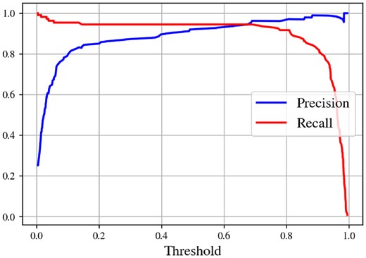
The precision and recall curves of the meta-learner on the validation set at different threshold values. Modifying the threshold value used for labelling the instances allows for improving performance in either precision or recall at the expense of the other, depending on which is prioritised.
When compared to the SVM and RF performance metrics in Table 7, it is clear that the basic model design substantially outperforms both when it comes to generalization over the holdout sets. Both the SVM and RF tend to overfit the first training set to a far greater degree, with metrics, especially the models’ recall (and by extension their F1 score), experiencing a sharp dropoff with the second training set and both holdout sets.
A final statistic we use to assess performance is the area under curve (AUC) score of the receiver operating characteristic (ROC) curves generated for the model on the different data sets. Table 11 lists the ROC–AUC scores for all four data sets, and Fig. 12 shows the ROC curve for the test set. The ROC curve is a graphical representation of the predictive strength of a binary classifier as the threshold value is varied. The straight diagonal line represents the ROC curve of a purely random classifier. As the elbow approaches the top left corner, the more ideal and predictive the binary classifier is, culminating in an AUC score of 100 per cent. With a score of 98.29 per cent on the test set, the model shows strong and clear signs of generalization, implying that although the first-level voters are themselves not ideal, the ensemble model still achieves relatively strong scores.
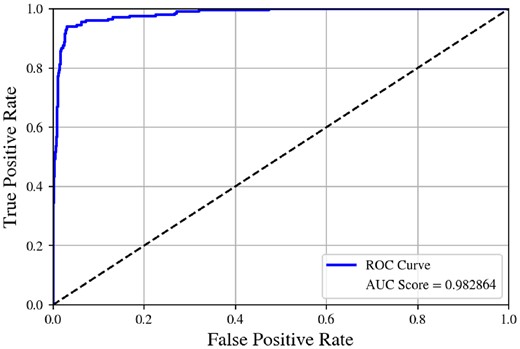
The ROC curve for the basic model on the test set.
ROC Area Under Curve (ROC-AUC) scores of the meta-learner in the basic model architecture set with a label threshold of 0.5.
| Data set | ROC-AUC |
|---|---|
| 1st level training set (%) | 99.82 |
| Meta-learner training set (%) | 97.92 |
| Validation set (%) | 98.01 |
| Test set (%) | 98.29 |
| Data set | ROC-AUC |
|---|---|
| 1st level training set (%) | 99.82 |
| Meta-learner training set (%) | 97.92 |
| Validation set (%) | 98.01 |
| Test set (%) | 98.29 |
5 AUTOENCODER BASE MODEL: DESIGN AND RESULTS
A relatively common technique used in ML applications (see Sharma et al. (2020) for a similar application to this work) is the application of semi-supervised learning to maximise performance during training and generalization.
The procedure is to first train the convolutional base of a deep network on an ideally sizeable unlabelled data set as part of an autoencoder. As described in Rumelhart, Hinton & Williams (1985) and shown in Fig. 13, autoencoders learn internal representations by applying error-propagation using the input features as the desired output. The architecture encodes the input to a compressed representation referred to as the latent space representation, then decodes this back to the original number of features. Hence, a perfect autoencoder essentially replicates an identity function on the data. In terms of convolutional autoencoders, the conventional approach is to compress the size of the feature maps gradually in the encoder either using pooling layers or non-unitary strides in the convolutional layers, while simultaneously increasing the depth of the instance. Therefore, at the latent representation, the spectrum would be in its most compressed and deepest form. This means that if this representation optimally preserves enough information from the original spectrum such that it can successfully reconstruct it, then it can provide means to reduce the dimensionality of the data (Hinton & Salakhutdinov 2006).
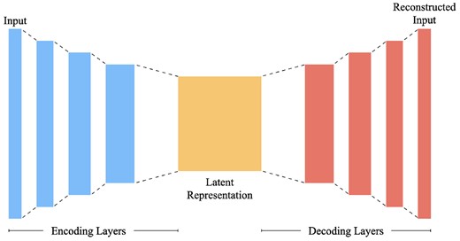
The autoencoder architecture.
Once the autoencoder is trained, the encoding layer is used as a convolutional base for the classifier as shown in Fig. 14. To do so, a dense network is appended to the trained convolutional base, and the weights of the latter are fixed. The labelled data set is now used to train the weights of the classifier, using the latent representation learned by the convolutional base to optimise and stabilise learning. With such a technique, the classifier will essentially need only learn the transformation function which separates the two classes, rather than needing to simultaneously learn the latent representation of the spectral input.

Semi-supervised transfer learning using convolutional autoencoders.
5.1 Preliminary motivations for design
Prior to any decisions regarding any specifics within the autoencoder and final classifier design of the first-level voters, an evaluation of the performance during training of the basic model provides worthwhile insight. As was concluded in Section 4.2, whilst the final ensemble collectively scores relatively high in most of the classification metrics considered, the model tends to be prone to overfit the training set on which the first-level voters were trained on. Furthermore, in the case of the first-level classifiers’ individual performance on the validation set, only 3 voters achieve substantial generalization whilst still overfitting to the first training set. Their minimization of the validation set was also prone to be quite unstable.
Hence, any improvements will ideally aim to stabilise learning and generalization, as well as allow for more voters to generalize more convincingly. It is important to note at this stage that the priority is not necessarily to solely achieve higher classification metrics. Whilst it is naturally a positive, care needs to be taken that during training and inference, the model is stable and reliable such that it is generalizable to instances beyond the training and holdout sets. This is especially true in this case due to the compromise of using multiple observations of the same target. Therefore, aiming to stabilise the model and achieve more consistent generalization should be given similar importance to strong metrics. To improve generalization and minimize overfitting for ML models, there are typically a number of changes that can be explored. The first is to incorporate stronger regularisation. The training techniques used and the model architecture should then be re-evaluated. In the case of CNNs, as the information becomes encoded in the deeper layers, a decrease in learning and generalization could imply a loss of information with further compression of the spectrum. Hence training the convolutional base in such a way as to optimise the transformation of the data as it becomes deeper and more compressed should allow for greater stability in its learning and generalization. If however none of the above prove to be definitively effective, then it may highlight the need for more training instances shown to the model, that is, increasing the size of the data set.
The apparent need for a different training regime, model architecture and larger data set could be met by incorporating the semisupervised learning techniques described previously. Primarily, the introduction of a new large unlabelled data set immediately enables the model to fit a greater diversity of training instances and approximate a more generalisable transformation function, whilst alleviating the need to label all samples as would be the case for fully supervised learning. Secondly, it is useful to train the convolutional autoencoder separately as a regression task with the unlabelled data set, rather than immediately using the labelled data set to train it in terms of binary classification. This allows for the opportunity for the convolutional layers to be trained to maximally preserve the spectral information during compression and increase in depth, enough for the spectrum to be substantially reconstructed by the decoder. Therefore, if the base is adequately tuned for this reduction in dimensionality prior to being exposed to the labelled data set, then the latent representation fed to the classifier from the convolutional base should be expected to be more stable, more representative, and less deteriorated in terms of the underlying information. Since during the supervised training of the classifier most of the convolutional base will not be trainable and have its weights fixed, then this also acts as a form of regularization by drastically reducing the number of trainable parameters. In conclusion, several of the issues present in the basic model’s performance can be minimised or alleviated entirely by incorporating semi-supervised learning with the convolutional base trained as part of an autoencoder beforehand.
5.2 System architecture
This section will describe the architecture employed for the convolutional autoencoder in which the convolutional base is trained, the final classifier design employed for the first-level voters and the meta-learner in the overarching ensemble classifier. Prior to that, we first introduce a further level of regularization incorporated into the model, namely kernel regularisers. Then, as the subsequent sections will explain, the task shifts from that of a regression task at the autoencoder stage, to a binary classification task once the classifier is complete. This means that different metrics and methods for performance evaluation are needed so that training can be reliably assessed.
5.2.1 Implementation of kernel regularization
After it was apparent that the first-level classifiers in the basic model design were overfitting to the training set, we revisited the model architecture to incorporate more methods of regularisation. Whilst Batch normalization is also present in the model, testing whether or not including kernel regularization helps the model to not overfit will clarify if a larger data set is necessary to dampen the fluctuating training curves.
Least Absolute and Selection Operator Regression (Lasso), originally proposed by Tibshirani (1996) is a form of regularized regression in which an additional term, containing the ℓ1 norm of the weight vector, is added to the cost function. Hence, for a weight vector θ, the cost function for an MSE regression problem becomes,
where λ1 acts as a regularisation factor. A particular strength of Lasso regression is to promote sparsity in the model by diminishing the weights of the least important features. In the case of spectral classification, it therefore warrants an exploration of whether this helps stabilize the fluctuating generalization in the model.
Ridge Regression (also known as Tikhonov or Tikhonov–Phillips regularization) applies a penalty term to the cost function incorporating the square of the ℓ2 norm of the weight vector. For a weight vector θ, the cost function for an MSE regression problem is hence given by,
where λ2 acts as a regularization factor. Ridge regression tends to minimize all weights in the model without entirely driving them to 0, essentially favouring bias in place of maximal variance. It is also known to alleviate multicollinearity effects for large-dimension problems. As the spectra themselves have a large number of features, introducing ridge regression could help in alleviating some degree of overfitting to the training set.
As both regularization methods tend to provide their own particular merits, both were implemented into the model during training. The explored values for the λ1 and λ2 hyperparameters are given in Table 12.
Explored values for the L1 and L2 regularization implemented into the autoencoder model and final first-level classifier design.
| Hyperparameter | Explored values |
|---|---|
| λ1 | 10−1, 10−2, 10−3, 10−4, 10−5, 0 |
| λ2 | 10−1, 10−2, 10−3, 10−4, 10−5, 0 |
| Hyperparameter | Explored values |
|---|---|
| λ1 | 10−1, 10−2, 10−3, 10−4, 10−5, 0 |
| λ2 | 10−1, 10−2, 10−3, 10−4, 10−5, 0 |
5.2.2 Autoencoder design
Partially motivated by the architecture presented in Sharma et al. (2020), we employ a similar convolutional autoencoder design, whilst following the traditional conventions used in the rest of the ML literature.
The encoder receives a 1D spectrum of shape (4174,1) and passes it through several convolutional blocks of kernel size 5, each progressively compressing the data while simultaneously increasing the depth. Compression was done directly through the convolutional layer itself, rather than with a pooling layer, simply by setting the stride to be equal to 2. In cases such as this where a certain level of spatial (or spectral) information could be expected to contribute to providing the optimal latent representation of the data, Chollet (2021) states that incorporating the compression into the convolutional layer and not implementing pooling layers helps reduce the spatial invariance introduced into the model. The depth (number of filters) is doubled with each convolutional block, culminating in a shape of (261, 256) at the encoded representation at the centre of the architecture. The stride of this block was set to 1, in order to attain a level of symmetry in the architecture before flowing into the decoder. The decoding layers subsequently deconvolve and decompress the spectrum back to its original input shape, through the use of 1D transpose convolutional blocks set with a stride of 2. We incorporate a number of cropping layers at certain points across the decoder to ensure that the final output of the architecture matches the shape of the input.
In order to allow for an arbitrarily deep autoencoder, we employ residual connections to each convolutional block as recommended in He et al. (2016). As neural networks get deeper and deeper, the vanishing/exploding gradient problem becomes more pertinent. Reformulating layers to be residual functions which take their input into account allows for easier optimisation and reduced occurrence of the aforementioned problem. With convolutional layers, this is implemented by passing the input not only through the typical convolutional & ReLU activation layers, but additionally through a separate parallel path with a convolutional layer of kernel size 1 and same number of filters as the alternate path. This allows the addition of the tensor output from the activation layer to the input of the block, both of which would be of the same shape.
Once built, the model was compiled & trained using an SGD optimizer, a learning rate of 0.0001, a mean square logarithmic error loss function and a batch size of 512 samples.
As was the case in previous designs, we incorporate regularisation techniques into our model. Firstly, every convolutional block includes a batch normalization layer before the activation layer, as recommended in Ioffe & Szegedy (2015). Furthermore, kernel regularizers are included for each convolutional layer, incorporating both ridge and lasso regression techniques as described in Section 5.2.1. The final design is shown in Fig. 15, and the explored values for the hyperparameters are given in Table 12.
5.2.3 Final classifier design
Once all autoencoder models were trained, the next immediate step was to use the trained encoder layers as part of the convolutional base of the first-level classifiers. We describe the process of transfer learning in Section 5 in its simplest terms, yet as was immediately evident in our application of the technique, certain modifications and additions in the architecture were needed to allow for minimization of the loss function, and by extension, learning & generalization.
Fig. 16 displays the final architecture employed for the classifier, where rather than the pre-trained encoder constituting the convolutional base, the deepest two convolutional layers of the encoder were replaced with two trainable convolutional blocks, one with two convolutional layers and the deeper block with one. As will be evident throughout this section, most of the design choices came directly from either the basic model results or from initial training runs using Bin_06 as a ‘test’ voter (the implications and ramifications of this will be discussed in Section 5.3.2 and Section 6). The modification choices were not based on the accuracy metrics of the classifier during training, but rather on the minimization of the training loss and stability of generalization.
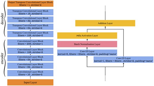
The autoencoder architecture employed in this work. The left diagram shows the general design, typical to conventional autoencoders found in the literature. A stride of 2 was used to compress (and subsequently decompress) the spectrum rather than a pooling layer, in order to avoid any unnecessary loss in spatial information. As the spectrum is encoded through compression, its depth is doubled with each convolutional block. The design of each convolutional block is presented in the image on the right-hand side. To allow the architecture to be arbitrarily deep and to mitigate the vanishing/exploding gradient problem, we employ residual connections. Batch normalisation is incorporated before the activation layer, and the output is then subsequently added to the residual connection. In the case of the transpose blocks, the convolutional layers are simply replaced with a transpose 1D convolutional layer.
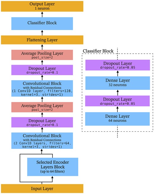
The pre-trained classifier architecture used for the first-level voters. The left diagram shows the general design, including the non-trainable encoder layers block connected to the input layer (with a residual connection), followed by two sets of trainable convolutional blocks. Each block feeds into a dropout layer and average pooling layer to handle regularisation and spectral compression, respectively. Finally, a flattening layer is used to prepare the intermediary input to be fed into a dense classifier architecture, which is described in the diagram on the right-hand side. The output layer finally outputs 1 neuron with a sigmoid activation function, such that the final output results in a probability score used to assign a label to the data instance.
Prior to discussing the reasons for the additions, it would be prudent to first justify the removal of the deepest two layers of the encoder. In the initial runs attempting to train the classifier, we observed a crucial issue: the model was not converging, and no minimization of the loss function was occurring. The depth of the encoder, particularly the two deepest layers, appeared to be a significant factor contributing to this problem. The majority of the pertinent information hidden within the spectra, which was crucial for distinguishing between the two classes, was being lost at the informational bottleneck created by these deep layers. This resulted in the model’s inability to learn and minimize the loss effectively. Therefore, we chose to omit the final two layers and instead use the shallower encoding, allowing the rest of the trainable convolutional block to work with a less compressed representation of the data.
An immediate issue that came up during initial training runs highlighted that with a simple serial connection of the selected pre-trained encoder layers, the training performance, in terms of the loss, was suggestive of the gradients ‘vanishing’ as the training epochs progressed. To alleviate this, we introduced a residual connection across the pre-trained block of layers. Similarly, within the proceeding blocks, it should be noted that all convolutional layers have the same residual connections as employed in the autoencoder design and the same choice of activation function. However, the number of strides is set to 1, since the compression will be handled using pooling layers. It should be noted that L1 & L2 regularisation was implemented for every convolutional layer, set to 0.01 and 0.001, respectively. Each convolutional block is followed by a dropout layer (with 10 per cent dropout) and an average pooling layer with a pool size of 2. The choice of an average pool, rather than a max pool, was done in order to minimize the loss of spatial (spectral) information during compression, a factor we considered upon reflecting on the performance of the basic model.
All the aforementioned layers collectively constitute the convolutional base of the model and are therefore followed by a flattening layer, to prepare the encoded representation of the spectrum to be fed through the dense classifier culminating in a prediction score. The classifier is composed of two hidden layers, with 64 and 32 neurons, respectively, and a softsign activation function. L1 and L2 regularization is also employed, with each of their alpha hyperparameters set as tunable values during the cross-validation stage. The explored values are the same as in the autoencoder stage, given in Table 12. Each dense layer is followed by a dropout layer with 5 per cent dropout. Finally, typical of any binary classification task, the final dense layer of the classifier has 1 neuron and a sigmoid activation function.
For reasons more to do with practicality and feasibility in terms of training time and computational load, the number of tunable hyperparameters beyond the initial training runs on Bin_06 was reduced compared to the basic model. The hyperparameter choices based on these initial runs include the alpha values of the L1 and L2 regularization of the trainable convolutional layers, and the choice of activation function of these dense hidden layers (The list of explored values for both hyperparameters is common to the meta-learner as shown in Table 13). This however implies that the first-level voters are more rigid across the different bins, and might therefore lead to a reduction in their adaptability to the bins they are being trained on.
Explored values for all model hyperparameters of the meta-learner for the autoencoder base model design.
| Hyperparameter | Explored values |
|---|---|
| n_dense_hl | 1, 3, 5 |
| n_neurons_first | np.arange(100, 750) |
| dropout_rate | 0, 0.1, 0.2, 0.25, 0.35 |
| l1_alpha | 10−1, 10−2, 10−3, 10−4, 10−5, 0 |
| l2_alpha | 10−1, 10−2, 10−3, 10−4, 10−5, 0 |
| activation_fn | ‘selu’, ‘elu’, ‘relu’, ‘tanh’, ‘softsign’ |
| optimizer_type | ‘adam’, ‘adagrad’, ‘nadam’, ‘sgd’ |
Once the entire first-level voter model was built it was then compiled, again implementing a binary_crossentropy loss function. The Adam optimizer was also used, this time with its starting learning rate set at 0.001. To expedite training and allow for the optimizer to minimise the loss function in a more stable fashion, an exponential learning rate scheduler is employed during training, such that the learning rate l at epoch n, is given by
where l0 is the initial learning rate and s is a hyperparameter signifying the number of epochs after which the learning should drop by an order of magnitude. For this model, l0 was set to 0.001 as previously mentioned, and s was set to 300 epochs.
Training then finally commenced with a batch size of 256 instances. The number of epochs was set to a maximum of 1000, incorporating early stopping with a patience value of 150 epochs.
5.2.4 Meta-learner design
The design of the meta-learner is mostly kept similar to that in the basic model design described in Section 4.1.2. However, some additional regularisation was included once it became apparent that the model was overfitting the second training set.
The first inclusion of regularisation attempts to force the classifier to learn representations which do not strongly depend on the strongest and most reliable voter, such that the final weights are then skewed heavily on that voter’s input. To do so, a dropout layer was introduced right after the input layer, such that during training certain input neurons were switched off to allow the model to optimize its representation based solely on the activated neurons at that point. The dropout rate was set with a tunable hyperparameter. Then, to incorporate regularisation into the dense layers, L1 and L2 regularisers were added for each of the hidden layers and subsequently tuned by their alpha hyperparameters. This meant that a total of 3 hyperparameters were added to the list pre-existing from the basic model design.
To tune the hyperparameters, we again used a randomised cross-validation search as was the case in Section 4. A 3-fold CV search was conducted over 50 permutations of the explored values listed in Table 13.
5.2.5 Control test with common classification methods
Since bar the selection of first-level voters the procedure for the generation of comparative metrics was the same for both models, the reader is referred to Section 4.1.3 for an explanation of how the results in Table 8 were obtained.
5.3 Training performance and results
As was the case with the basic model, evaluating the ensemble classifier’s performance should be split two-fold, an individual assessment of training performance and validation tests on the first-level voters, and a final analysis of the meta-learner performance on all the training and holdout sets. However, as the first-level classifiers are trained in a semi-supervised learning regime, this requires additional evaluation of the performance of the autoencoder model on the unlabelled training & validation sets.
5.3.1 Performance of autoencoder
As mentioned in Section 5.2, the unsupervised learning task of training the autoencoder model to the unlabelled data set is treated as a regression task. An important point to repeat prior to commenting on any of the performances is that the purpose of the autoencoder architecture is to achieve a compressed, latent representation which preserves most of the underlying signal within the data. Essentially, this amounts to attaining an optimal dimensionally reducing transformation function at the encoder stage of the model. Hence, as the decoder is then attempting to reconstruct the spectrum as closely to the original input, the classification task, for which it will later have some of its convolutional layers used, is irrelevant at this stage. Here it is not important whether or not there are any ‘planetary formation markers’ within the range of bin for each particular model. Each model is attempting to optimise the best latent representation for their assigned spectral range, which means that all 25 bins should be expected to learn and generalize well.
Fig. 17 shows the training performance of all 25 autoencoder models in terms of the mean square logarithmic error on the training and validation set at every training epoch. The regularisation hyperparameters, namely the L1 and L2alpha values, are listed for each model.
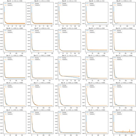
The mean square logarithmic error of the autoencoder models on the training and validation set at every training epoch. All 25 models are shown and labelled accordingly, and the alpha hyperparameter settings for the L1 and L2 regularization are given.
As expected, all training curves demonstrate strong and stable minimization of the loss function, with most models only requiring ∼50 epochs for both the training and validation curves to start to plateau. The validation loss tends to be convergent with the training loss in most cases, albeit with varying degrees of regularisation. However, there are some notable cases in which training was slightly less successful than the best performers.
Bin_09’s best-performing model displays some overfitting, to a relatively small, but none the less significant, degree. Whilst L1 = 0.01 and L2 = 0.01 was the best-performing set of hyperparameters, introducing stronger regularisation resulted in significant deterioration of training and generalization, to the point where the model failed to minimize the training loss at all.
Bin_13 proved to be the worst performer out of the 25, with the validation curve plateauing at a loss almost double that of the other models. The training curve was also not fully minimized by the time early stopping halted training, clearly showing a divergence between the two curves and exhibiting signs of overfitting even with strong regularisation. It may be possible that the latent representation, in this case for this spectral range, is not representative of one which is truly generalisable, but heavily biased to the training set. We suggest that in future work, the model architecture choices specifically for this spectral range should be revisited and amended, such that a simpler model design would make it more regularisable. This could be a way in which a more generalized latent representation is achieved.
Bin_25, whiles overall not drastically overfitting the training set (similar in scale to that in the case of Bin_09) provides a validation curve that is significantly noisier and less stable than the rest. A plausible cause for this is instrumental noise at the extremities of the observed spectrum, which is to a lesser degree present in noticeable fluctuations in the validation curve of the Bin_01 autoencoder. As the majority of instances in the data set are ESO-HARPS spectra, whose range starts and ends with Bin_01 and Bin_25, respectively, this should tend to introduce a significant source of noise within both ranges. A future improvement could be to introduce a larger proportion of ESO-FEROS spectrum into the unlabelled data set, so as to allow for the models to more substantially learn to represent the spectral ranges’ latent representations effectively with less pronounced effects from the introduced noise.
5.3.2 Performance of classifiers
With the autoencoders trained on the unlabelled data set, the lower layers of the encoder were used in the architecture of the new first-level voter design, as described in Section 5.2.3.
An immediate improvement over the basic model design was the drastic increase in responsive voters, rising from 3 to 20. Table 14 displays each of their wavelength ranges, the best-performing model’s accuracies on the first training set and validation set and the model weights and rank assigned by the first layer in the meta-learner. Whilst several amendments were made from the basic model, it is likely that this increase in response comes from the pre-trained layers at the shallow end of the classifiers. As the unsupervised training attempted to converge to a latent representation which maximises the preservation of the signal in the spectrum, the inclusion of some of the encoding layers allows the classifier to learn a generalisable transformation function without needing to train and tune the shallow layers. It should be noted that when simply looking at the accuracy metrics for the 3 common responsive bins, there is a substantial drop in performance compared to the basic model design. However, the pre-trained model has far stronger regularisation applied to it, which was not the case for the basic model. Furthermore, as demonstrated in the training curves, the best-performing model does not manifest itself through a sharp and erratic fluctuation but instead follows a more stable minimization of the loss function.
The twenty responsive first-level classifiers for the pre-trained base model architecture. The bins marked with an * are those which were responsive for the basic model design described in Section 4. To quantify the influence of each of these first-level voters in the aggregated score provided by the meta-learner, the final column presents the model weight magnitudes of the first layer in the meta-learner. Higher weight magnitudes tend to give a general indication of which input features (i.e. first-level classifier scores) the meta-learner tends to favour.
| Best model accuracy (%) | |||||
|---|---|---|---|---|---|
| Bin name | Wl range (Å) | 1st training set | Val. set | Meta-learner first layer weight mag. (Rank) | |
| Bin_02 | |$3907.17^{+0.85}_{-0.69}$| | |$4032.36^{+0.85}_{-0.69}$| | 89.36 | 85.92 | 1.03418 (17th) |
| Bin_03 | |$4032.39^{+0.85}_{-0.69}$| | |$4157.58^{+0.85}_{-0.69}$| | 93.66 | 89.92 | 1.37128 (5th) |
| Bin_04 | |$4157.61^{+0.85}_{-0.69}$| | |$4282.80^{+0.85}_{-0.69}$| | 92.15 | 90.34 | 1.28191 (9th) |
| Bin_05 | |$4282.83^{+0.85}_{-0.69}$| | |$4408.05^{+0.85}_{-0.69}$| | 90.94 | 89.29 | 1.00672 (19th) |
| Bin_06* | |$4408.05^{+0.85}_{-0.69}$| | |$4533.24^{+0.85}_{-0.69}$| | 91.50 | 88.45 | 1.00704 (18th) |
| Bin_07* | |$4533.27^{+0.85}_{-0.69}$| | |$4658.46^{+0.85}_{-0.69}$| | 93.17 | 90.13 | 1.25590 (11th) |
| Bin_09 | |$4783.71^{+0.85}_{-0.69}$| | |$4908.90^{+0.85}_{-0.69}$| | 92.58 | 90.76 | 1.54970 (4th) |
| Bin_13 | |$5284.59^{+0.85}_{-0.69}$| | |$5409.78^{+0.85}_{-0.69}$| | 87.69 | 86.34 | 1.14412 (13th) |
| Bin_14 | |$5409.78^{+0.85}_{-0.69}$| | |$5535.00^{+0.85}_{-0.69}$| | 85.13 | 84.46 | 1.22386 (12th) |
| Bin_15* | |$5535.03^{+0.85}_{-0.69}$| | |$5660.22^{+0.85}_{-0.69}$| | 93.07 | 90.13 | 1.68282 (2nd) |
| Bin_16 | |$5660.25^{+0.85}_{-0.69}$| | |$5785.44^{+0.85}_{-0.69}$| | 84.01 | 82.36 | 1.36227 (6th) |
| Bin_17 | |$5785.47^{+0.85}_{-0.69}$| | |$5910.66^{+0.85}_{-0.69}$| | 95.44 | 92.65 | 1.76358 (1st) |
| Bin_18 | |$5910.69^{+0.85}_{-0.69}$| | |$6035.91^{+0.85}_{-0.69}$| | 93.20 | 88.66 | 1.30675 (8th) |
| Bin_19 | |$6035.91^{+0.85}_{-0.69}$| | |$6161.10^{+0.85}_{-0.69}$| | 87.66 | 85.71 | 1.12453 (14th) |
| Bin_20 | |$6161.13^{+0.85}_{-0.69}$| | |$6286.32^{+0.85}_{-0.69}$| | 92.06 | 90.13 | 1.25642 (10th) |
| Bin_21 | |$6286.35^{+0.85}_{-0.69}$| | |$6411.54^{+0.85}_{-0.69}$| | 91.46 | 89.50 | 1.04212 (16th) |
| Bin_22 | |$6411.57^{+0.85}_{-0.69}$| | |$6536.76^{+0.85}_{-0.69}$| | 89.69 | 89.29 | 1.31345 (7th) |
| Bin_23 | |$6536.79^{+0.85}_{-0.69}$| | |$6661.98^{+0.85}_{-0.69}$| | 89.40 | 87.40 | 1.06683 (15th) |
| Bin_24 | |$6662.01^{+0.85}_{-0.69}$| | |$6787.20^{+0.85}_{-0.69}$| | 95.01 | 89.50 | 1.66936 (3rd) |
| Bin_25 | |$6787.23^{+0.85}_{-0.69}$| | |$6912.415^{+0.85}_{-0.69}$| | 87.20 | 86.34 | 0.99848 (20th) |
In the training plots shown in Figs 18 and 19, it is immediately evident that there is an increase in stability in the validation loss. Even in the accuracy curves, the validation accuracy tends to demonstrate less erratic behaviour, albeit still exhibiting a level of milder fluctuation for most bins. A contrast that is important to point out is the number of epochs for which training was allowed to be carried out. For the basic model design, training struggled to go beyond 200 epochs, as the validation loss quickly plateaued and diverged from the training loss. This meant that early stopping was invoked at relatively early stages of training because the model showed no further signs of minimization and was starting to overfit to the training set. In the pre-trained model training runs, however, early stopping was invoked at far higher epochs because the model continued to minimize the validation loss. Now, this can be attributed to a number of choices in the model design and training regime. Firstly, the pre-trained layers offer a form of regularisation in that they are not trainable. This means that the lower encoding of the spectrum is already learned, and allows the parameter tuning to focus on the higher-level abstraction in which we expect the class-determining features to be manifested. Secondly, adding residual connections not only within the convolutional blocks but across the pre-trained layers allows for less information within the model to be lost during back-propagation, regardless of the depth. The implementation of a scheduler also provides a more stable training regime, ensuring that in later epochs the model does not erratically escape a region of the parameter space in which it demonstrates minimal loss.
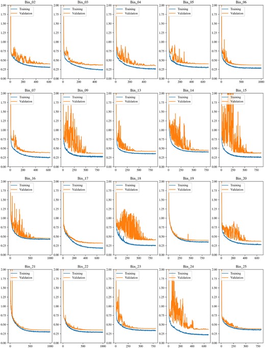
The training and validation loss of the 20 responsive first-level classifiers.
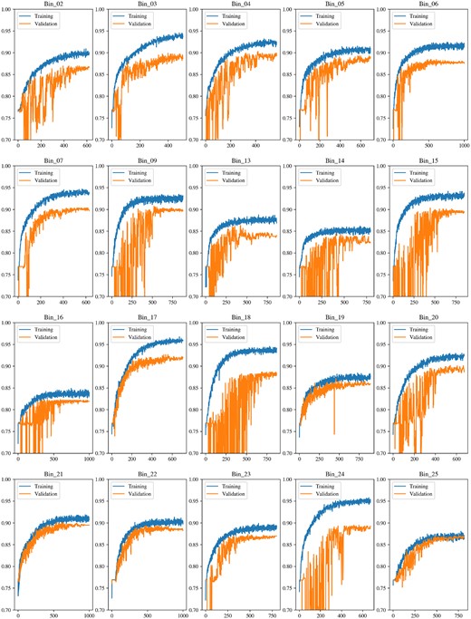
The training and validation accuracy of the 20 responsive first-level classifiers.
That being said, it is clear that for most bins, the models still are prone to overfit the data, with varying degrees of severity. Early to mid-stage epochs for several models tend to show a certain level of fluctuation in the validation curves, even though the validation loss still tends to minimise when observing its trend in a general sense. Furthermore, models for certain bins, notably Bin_15, Bin_18 and Bin_24, have training and validation accuracy curves which tend to immediately diverge and demonstrate clear signs of overfitting. This is likely in part to be an artefact from tuning the regularisation parameter to the initial training runs for the Bin_06 model, and even though this hyperparameter tuning was done with care in terms of the extent of it, there is still an element of rigidity introduced which hinders generalisability. It brings further concern when taking into account that Bin_15 and Bin_24 have weight magnitudes which rank 2nd and 3rd, respectively. We, therefore, suggest that in future work, more time is spent tuning the model hyperparameters for each bin separately, such that these instances of overfitting can be reduced. It should be highlighted again however that relative to the basic model, the responsive classifiers all show far more stable signs of generalisability in their learning. Before, the erratic nature of the training plots and lack of response from several bins suggested that the model architecture requires modification. The level of overfitting now, rather than requiring more immediate model regularisation, can also be indicative of the inherent noise within the spectral input. This could be tested by restricting the data set to one of higher SNR, or by introducing more intensive noise reduction techniques during the pre-processing stage. Thus, the suggestion for future improvement can be viewed to have shifted more toward the data set rather than the model architecture.
5.3.3 Performance of meta-learner
Mirroring the process of the basic model, with all first-level voters fully prepared, the focus was switched to training the meta-learner on the second training set. This section aims to assess its performance on the training and holdout sets independently, in what the performance metrics seem to suggest about its learning and generalization, and then within the context of the basic model’s performance. The performance metrics are presented in Table 15, set for the default threshold of 0.5 and a custom threshold of 0.4 based on the precision and recall curves.
Performance metrics of the meta-learner in the pre-trained base model architecture set with a labelling threshold of 0.5 and 0.4.
| Data set | Accuracy | Precision | Recall | F1 score |
|---|---|---|---|---|
| Threshold set to 0.5 | ||||
| 1st level training set (%) | 98.69 | 99.11 | 95.16 | 97.10 |
| Meta-learner training set (%) | 94.78 | 92.89 | 83.76 | 88.09 |
| Validation set (%) | 92.65 | 85.05 | 82.72 | 83.87 |
| Test set (%) | 94.19 | 92.17 | 81.68 | 86.61 |
| Threshold set to 0.4 | ||||
| 1st level training set (%) | 98.78 | 98.54 | 96.15 | 97.33 |
| Meta-learner training set (%) | 94.38 | 90.04 | 85.04 | 87.47 |
| Validation set (%) | 92.23 | 83.48 | 82.72 | 83.11 |
| Test set (%) | 93.85 | 88.94 | 83.66 | 86.22 |
Focusing on the 0.5 threshold results, it can be seen that when looking at the metrics for the first training set, meaning the data set used to train the first-level voters individually, the combined model through the aggregated score of the meta-learner, manages to outperform the accuracy score achieved by every responsive first-level voter in Table 14 by at least 3 per cent. This was also the case for the basic model. It suggests that the vote aggregation occurring through the meta-learner allows for a collectively stronger performance when considering the whole spectrum rather than individual bin ranges. Consider that for one instance, a usually well-performing voter lacks clarity in the spectral features/patterns within its bin which have been deemed class-defining, and hence results in a more tentative prediction score. The meta-learner is showing preliminary evidence for being able to put this less resolute score in context with the other voters looking at different spectral ranges, such that the final aggregated score ends up being more reliable.
Shifting to the metrics for the second training set, i.e. the data used to train the meta-learner, there is a drop in performance from those of the first training set. However, this is to be expected to a degree, as the second training set is not being seen by the model in its true input representation, but rather through the interpretation of the first-level voters. Hence, as these are all tuned and trained with respect to the first-level classifiers, then it should be expected that the meta-learner’s interpretation will be influenced by that. The accuracy and F1 scores drop off slightly from that in the basic model, and the precision increases whilst recall significantly dips. This can be adjusted in terms of the trade-off when customising the labelling threshold, but care needs to be taken when doing so.
The validation scores easily see the biggest drop-off, especially when compared to those seen in the basic model metrics. The resultant confusion matrix,
shows 16 false positives and 19 false negatives. Whilst initially these can all be viewed as a negative when compared to the previous model, it does suggest that during this run of training, the hyperparameters were not overfitting the validation set during model design and cross-validation. This concern can be retrospectively levelled on the basic model, considering that the validation set significantly over-performs the second training set in Table 10. As described in Section 5.2, the validation set was not used for hyperparameter tuning to the same extent during the pre-trained base model training. It was used to test the initial architecture choices for the Bin_06 model and beyond that only sparingly to tune the alpha hyperparameters for the L1 and L2 regularisation for the other voters. For the basic model design, the validation set was used more extensively during the hyperparameter tuning stage.
Finally, performance on the test set, whilst worse than the basic model score, maintains a similar performance to that seen by the second training set, with a 94.19 per cent accuracy. The recall is noticeably lower, resulting in an F1 score. The confusion matrix is
Again, these can be marginally improved by manipulating the labelling threshold value and instigating a trade-off with the model’s precision. However, the scores here seem to show fewer signs of overfitting to the second training set, and whilst the generalization is scoring less, the evidence from the performance during training and evaluation of the first-level voters suggests that it is more stable than that of the basic model.
As was discussed above when commenting on the degradation in the model’s recall, the threshold value used for assigning labels to the final prediction scores can be manipulated with care, especially when handling imbalanced data sets such as in this case. Precision and recall curves against the threshold value can be generated for the validation set to help inform this choice, as was done previously and as is shown for this iteration of the model in Fig. 20. The trade-off between precision and recall can be seen as the curves intersect close to a threshold of 0.4. To illustrate the change in performance, we present the metrics for the model with a threshold set at 0.4 in Table 15. As can be seen, the recall score for all data sets sees an increase, at the expense of precision. The first training set is the only one, however, to see this result in a very slight increase in its accuracy and F1, as the rest see a sharper decline in precision. Hence, care is suggested whenever customising the threshold value.
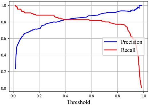
The precision and recall curves of the meta-learner on the validation set at different threshold values. Modifying the threshold value used for labelling the instances allows for improving performance in either precision or recall at the expense of the other, depending on which is prioritised.
When consulting the SVM and RF performance metrics in Table 8, as was done for the basic model, similar conclusions can be drawn for the autoencoder base model. The generalization displayed by our model significantly improves on the performances of both methods. To the point, the RF system of voters tends to overfit the two training sets and exhibits a sharp drop in recall over the holdout sets, whilst the SVM iteration suffers from low recall even on the training sets. Comparatively speaking, our model shows greater stability over its performance on the holdout sets, albeit the tendency to overfit the first training set is not alleviated.
Finally, the ROC curves and their AUC scores presented in Table 16 can allow for an alternative measure of performance. Taking a look at the ROC curve in Fig. 21 for the test set, the model scores an AUC of 96.51 per cent. Whilst still lower than the basic model, as is the case for every data set other than for the first training set, the model still achieves what appears to be strong generalization.
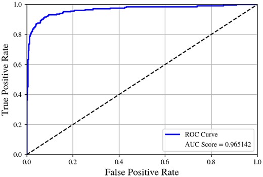
The ROC curve for the pre-trained base model on the test set.
ROC area under curve scores of the meta-learner in the pre-trained base model architecture.
| Data set | ROC-AUC |
|---|---|
| 1st level training set (%) | 99.86 |
| Meta-learner training set (%) | 97.02 |
| Validation set (%) | 96.01 |
| Test set (%) | 96.51 |
| Data set | ROC-AUC |
|---|---|
| 1st level training set (%) | 99.86 |
| Meta-learner training set (%) | 97.02 |
| Validation set (%) | 96.01 |
| Test set (%) | 96.51 |
To conclude, it seems evident that for the model to boost its generalisability, further information needs to be shown to not only the first-level voters but also directly to the meta-learner. We suggest possible additions in the following section.
6 DISCUSSION AND FUTURE WORK
In this work, we attempt to develop and test a binary classifier capable of discriminating between the stellar spectra of gas-giant hosts and comparison stars, motivated by several bodies of work demonstrating observational and theoretical evidence for chemical differences between the two populations. To do so, we curate two data sets of ESO spectra from the HARPS and FEROS instruments at the La Silla facility, culminating in a labelled data set of 5417 samples and an unlabelled data set of 25 168 samples. These were used to train, tune and test two different ensemble models in which the full spectrum was split into 25 disjoint bins. The first-level voters in the first model had a simple, conventional CNN design, and were fully trained on the labelled data set. In the second model, the shallow layers were first trained in a convolutional autoencoder design using the unlabelled data set. These layers were then incorporated into the final design and the rest of the layers were tuned using the labelled data set as was the case with the first model. The meta-learner in both cases was trained using the prediction scores from all responsive first-level voters as input.
Prior to any discussion regarding results, it is important to revisit a caveat and limitation in the data curation stage. Since the decision was taken to have multiple spectral observations of the same target star serve as separate data samples across different subsets in the data set, all results need to be assessed conservatively. As explained in Section 3.4, for the limited number of stars represented in the global data set, even more so for the number which would be present in the test set if the star samples were disjoint across the data sets, interpretation of the generalization scores of the model would be less dependent on the model performance, as stellar astrophysical biases would be more severe. Hence persisting with an instance-independent stratified sampling strategy was favoured for this iteration of the data set. Whilst this will lead to inherent bleeding of information across the data subsets, and hence reduce the stability of expected generalization on other samples external to those in the curated data set, it should also be noted that there is significant augmentation of each observation due to the inherent spectral noise (the strength of which varies) and artefacts of instrumental noise. The latter is particularly the case since data from two separate facilities was included. Hence, strong results should still indicate a level of generalization and applicability, even though the results should be conservatively assessed.
As the results for both models show, the meta-learner achieves relatively strong learning and generalization in both approaches, significantly outperforming the SVM and RF control tests. The basic model, whilst there are several concerns that will be reiterated below, manages to score relatively high in all performance metrics. Its generalization over the test set tends to be relatively stable, maintaining a high ROC-AUC score as well as a high recall and F1 score. The pre-trained model attempts to fix many of the issues within the performance of the basic model, especially in the first-level voter stage. Whilst the meta-learner performs worse than the basic model in the final metrics, the overfitting which was heavily present in the first-level voters was reduced with the introduced regularisation techniques. The minimization of the validation loss was also shown to be more stable, allowing for the introduction of stronger L1 and L2 regularization without learning degrading entirely. The new design resulted in a large increase in responsive classifiers, rising from 3 to 20. We aim to investigate the responsive spectral regions in future work. Shifting back to the meta-learner results, they still display relatively strong scores, even though recall suffers significantly from the basic model performance. Also, the performance suggests less overfitting to the validation set, which is explained by the reduced dependence on validation scores during the hyperparameter tuning stage. Hence, considering that the increase in stability and reduced overfitting when training the first-level voters, added to the fact that the overall meta-learner performance in terms of learning and generalization does not degrade tremendously, it can be argued that the pre-trained design has greater reliability in its ability to generalize over other samples beyond the test set.
When cross-examining the meta-learner model weights in both cases, it should be noted that out of the 3 common bins, Bin_06 is assigned a smaller magnitude in both cases. However, while Bin_07 is marginally prioritized in the basic model over Bin_15, the latter becomes substantially more important for the autoencoder base model, ranking second below Bin_17. The reason for this we suggest could be two-fold: either the meta learner in the second model, due to there being more responsive first-level voters present, is exposed to a fuller picture of the spectrum, and can therefore prioritise the scoring on Bin_15 based on the combined contribution of other voters not considered in the basic model. The second reason could be simply due to more stable learning thanks to the pre-trained layers and regularisation, which would lead to greater stability in the bin’s input feature during the meta learner’s training. This would lead to the model weights inherently adjusting to place greater priority on Bin_15’s scoring when aggregating the final score. Further work is required to fully understand whether this boost in preference is physical in nature or rather simply a byproduct of the training procedure.
There are, however, some caveats and significant concerns that arise out of both models’ performances. The basic model seems to show signs of overfitting the validation set, which might suggest that for future work, the training methodology should be improved with this in mind. Whilst it is valuable to use validation sets to tune model hyperparameters during training, care needs to be taken so that the model doesn’t end up overfitting to the validation set. Using the same validation set for the cross-validation hyperparameter tuning of all first-level voters, as well as for the meta-learner, can be a major source of the apparent overfitting of the basic model. For future work, it would be more prudent to either limit the extent of hyperparameter tuning with the same validation set (as was done for the pre-trained model) or split it into two disjoint subsets to be used for the first-level classifier training and meta-learner training separately. Beyond this, it should be reiterated that the first-level voters were very unstable in their minimization of the validation loss, and only 3 led to a clearly generalisable transformation function. Therefore the strong performance metrics should be conservatively assessed in their strength in generalization beyond this data set. The pre-trained model does fix several issues present in the basic model, however, there is still a degree of overfitting present, especially in the first training set. The main limitation in its ability to maximally learn from the second training set, at the stage where the meta-learner is implemented, is that at this level it is no longer directly viewing the spectral information, but rather the prediction scores administered by each responsive first-level voter. Hence, any future iterations of the model should include some form of direct spectral information fed to the meta-learner to maximize its ability to learn and generalize the distinction between the two classes.
The issues which persisted through the pre-trained model are not necessarily solely indicative of issues with the network architecture, but rather can highlight improvements to the input design and the data set itself. The overfitting present throughout the performance, even with strong regularization, could be an issue stemming from the inherent high presence of noise within the spectral input. Ground-based spectra are notoriously noisy due to atmospheric and thermodynamic effects, which should be expected to have an effect on limiting the strength of the generalization of any ML model. Solving this can be two-fold. The selection rules when curating the data set could be more restrictive in the allowed SNR values for the chosen spectra. Care needs to be taken when doing so, due to the trade-off between restricting the SNR distribution and ensuring that the final size of the data set is sufficient. Another solution could be to introduce denoising techniques in the pre-processing stage. However, the nature and strength of this need to keep in mind that the majority of spectral information important to discriminate between the two classes should be expected to be subtle. Hence, it is important that any denoizing procedure does not result in removing the ‘planetary markers’ from the spectrum entirely.
To alleviate the bleeding of information that is occurring due our stratified sampling strategy, future iterations of the data set will need to maximize the number of target stars present in the sample, such that the stellar diversity is high enough to allow for disjoint training and holdout sets without incorporating biases which may mask model performance.
Another issue that is important to acknowledge is that the training labels themselves are not definitive. Labels were assigned by reviewing several exoplanet archives for confirmed discoveries, and were compiled methodically and empirically. However, it is possible, and expected to be likely, that a number of comparison stars labelled to not host gas giant companions actually have an as-of-yet undiscovered gas giant companion. This implies the labelled data set is not entirely clean, and will need re-evaluating in the future to assess whether any comparison stars are in fact hosts.
Summarizing the planned future work we mention throughout this section:
We plan to analyse the responsive spectral regions of the pre-trained model, to suggest which spectral lines, and their presence/absence in the spectra, might be the source of the class-discriminating features.
Fixing the overfitting issue should be the main concern for the next iteration of the model. This will require amendments to the model architecture, input design, and the data set itself.
7 CONCLUSION
In conclusion, this work attempts to develop a binary classification model capable of discriminating between gas giant host and comparison star, and whilst there are still some persisting issues with overfitting, the model achieves stable and relatively strong generalization to suggest that future improved versions can lead to a reliable recommendation engine which can be deployed to suggest candidate stars for follow-up observation for gas giant detection.
Acknowledgement
The authors would like to thank the Institute of Space Sciences and Astronomy and the Faculty of Science at the University of Malta for providing access to computational facilities at the Ultrawideband Laboratory.
This work is based on observations collected at the European Organisation for Astronomical Research in the Southern Hemisphere under several ESO programmes.10 This research has also made use of the National Aeronautics and Space Administration (NASA) Exoplanet Archive, which is operated by the California Institute of Technology, under contract with the National Aeronautics and Space Administration under the Exoplanet Exploration Program. We would further like to acknowledge the use of the ExoKyoto Exoplanet Archive, developed & maintained by Kyoto University. The research shown here acknowledges the use of the Hypatia Catalog Database, an online compilation of stellar abundance data as described in Hinkel et al. (2014), which was supported by NASA’s Nexus for Exoplanet System Science (NExSS) research coordination network and the Vanderbilt Initiative in Data-Intensive Astrophysics (VIDA).
DATA AVAILABILITY
The data underlying this article were accessed and compiled from observations collected at the European Organisation for Astronomical Research in the Southern Hemisphere, accessed through the ESO Science Archive Facility.9 The unique identifiers of all observation files incorporated into both data sets can be found in https://github.com/miguel-zammit-uom/Jupiter-host-classification. The derived data generated in this research will be shared upon reasonable request to the corresponding author.
Footnotes
The observation IDs of all samples in the labelled and unlabelled data sets can be found in https://github.com/miguel-zammit-uom/Jupiter-host-classification
The list of all ESO programme IDs can be found in https://github.com/miguel-zammit-uom/Jupiter-host-classification
