


ABSTRACT
The growth of active galactic nuclei (AGNs) occurs under some form of obscuration in a large fraction of the population. The difficulty in constraining this population leads to high uncertainties in cosmic X-ray background and galaxy evolution models. Using an SDSS–WISE cross-match, we target infrared luminous AGN (W1 − W2 > 0.8, and monochromatic rest-frame luminosity above λLλ(12 μm) ≈ 3 × 1044 erg s−1), but with passive galaxy-like optical spectra (Optically Quiescent Quasars; OQQs). We find 47 objects that show no significant [O iii]λ5007 emission, a typically strong AGN optical emission line. As a comparison sample, we examine SDSS-selected Type 2 quasars (QSO2s), which show a significant [O iii]λ5007 line by definition. We find a 1:16 ratio of OQQs compared to QSO2s, suggesting that the OQQ duty cycle is likely much shorter than that of QSO2s (though selection biases are not fully quantified). We consider observed properties in comparison with other galaxy types, and examine them for consistency with theories on their intrinsic nature: chiefly (a) a high covering factor for surrounding obscuring matter, preventing the detection of high-ionisation emission lines – ‘cocooned AGN’; or (b) ionized gas being absent on the kpc scales of the Narrow Line Region (NLR), perhaps due to a ‘switching on’ or ‘young’ AGN. OQQs do not obviously fit the standard paradigm for merger-driven AGN and host galaxy evolution, implying we may be missing part of the flow of AGN evolution.
1 INTRODUCTION
The census of active galactic nuclei (AGNs) is, at present, highly incomplete. Dusty gas that feeds supermassive black hole growth can obscure the nucleus, resulting in an attenuation of AGN signatures along the line-of-sight (l.o.s.). This is not a minor effect: the majority of AGN are affected by obscuration. There are many lines of evidence pointing to this. Studies of the cosmic X-ray background radiation require obscuration by neutral gas with column densities (NH) exceeding 1022 cm−2 with between 2–5 as many times obscured AGN as unobscured ones (e.g. Setti & Woltjer 1989; Fabian & Iwasawa 1999; Gandhi & Fabian 2003; Gilli, Comastri & Hasinger 2007; Treister, Urry & Virani 2009; Ueda et al. 2014; Ananna et al. 2019). In the optical, obscuration can successfully explain the variety of observed AGN classes. Optical Type 1 AGN show broad emission lines with widths of several thousand km s−1 arising on scales of ∼ 30 |$L_{5100}^{0.7}$| light-days, where L5100 is the continuum rest-frame luminosity at 5100 Å in units of 1044 erg s−1 (e.g. Kaspi et al. 2000). Observing these close nuclear scales requires an extinction-free l.o.s.. Type 1 and Type 2 AGN show narrower emission lines with widths of a few hundred km s−1, which arise on scales of tens to thousands of pc. This difference in appearance can naturally be explained by an anisotropic distribution of dust which obscures the close-in broad lines, but not the larger scale narrower ones. In this way, the zoo of AGN classes can be unified. This model can also explain observed polarization fractions of broad emission lines (e.g. Antonucci & Miller 1985; Peterson 1997). In the radio, the radio-loud.1 subset of obscured quasars (‘radio galaxies’) was the first significant population of powerful and heavily absorbed AGN to be followed up in detail (e.g. McCarthy 1993; Miley & De Breuck 2008; Toba et al. 2019); many X-ray studies have now shown them to be strongly obscured, on average (e.g. Gandhi, Fabian & Crawford 2006; Tozzi et al. 2009; Wilkes et al. 2013).
The column density and geometry of obscuring matter are expected to naturally evolve as AGN and their host galaxies grow, and many models posit that the bulk of supermassive black hole growth occurs in highly obscured phases (e.g. Fabian 1999; Di Matteo, Springel & Hernquist 2005; Hopkins et al. 2006). AGN are also known to appear to change classification over time, from Type 1 to 2 and vice versa (Yang et al. 2018). These objects, referred to as ‘Changing Look’ AGN, show changes in emission line and continuum flux over timescales up to a few years. The physical mechanisms behind these changes are not well understood: the two main theories are variation in the line-of-sight obscuration (e.g. a clumpy torus; Elitzur 2012), a change in the accretion rate (e.g. Sheng et al. 2017), or thermal changes in the inner accretion disc (e.g. Stern et al. 2018). Any unusual AGN appearance must be considered in this context – lack of emission lines could be a transitional state of changing obscuration, or a change in intrinsic line production. Objects in the process of ‘switching on’ are a rare, brief chapter in the growth of AGN, an important but not well understood period. Sources with extreme covering factors approaching unity could also probe a unique phase in AGN evolution, indicating either strong growth rates with plenty of available circumnuclear matter for accretion or perhaps sky covering as a result of merger-driven turbulence. Several studies have linked galaxy mergers with higher rates of obscured AGN in MIR selected samples (e.g. Glikman et al. 2012; Satyapal et al. 2017; Weston et al. 2017). Although Seyfert galaxies with high covering factors approaching unity have been inferred in detailed individual studies (Ramos Almeida et al. 2009), the fraction of highly covered AGN at high power is expected to be small (e.g. Toba et al. 2014; Stalevski et al. 2016, although the dependence on luminosity is weak and not without counter-evidence – e.g. Netzer et al. 2016). Theoretically, accretion from large scales is not expected to be isotropic and is likely to be mediated via discs, warps, and other instabilities (e.g. Hönig 2019).
The infrared regime is particularly effective for studies of AGN dust covering factors, and for studies of AGN with absorbed optical signatures. This is because dust serves as a bolometer, absorbing and reprocessing the AGN power to the mid-infrared (MIR), providing a probe of the obscuring material in emission, as opposed to the absorption pathway provided in optical and X-ray studies. High angular resolution multiwavelength studies suggest that the MIR emission is effectively (to within a factor of a few) isotropic (Gandhi et al. 2009; Levenson et al. 2009; Asmus et al. 2015; Stalevski et al. 2016). Covering fractions derived from MIR AGN number counts and modelling of individual spectral energy distributions may also be a function of luminosity (Maiolino et al. 2007; Alonso-Herrero et al. 2011; Assef et al. 2013; Toba et al. 2013, 2014; Toba et al. 2021), though this remains controversial (Lawrence & Elvis 2010; Roseboom et al. 2013; Assef et al. 2015).
One limitation of most works on covering fraction to-date is the requirement for the presence of AGN emission lines (typically forbidden lines from the Narrow Line Region; NLR) in the optical or near-infrared, used to confirm the presence of an AGN and/or redshift identification. If AGN emission lines are observed, this implies that some intrinsic power must be escaping the AGN environment and the source cannot be fully covered. The presence of dust in AGN NLRs has been known for some time (e.g. Netzer & Laor 1993; Haas et al. 2005; Netzer et al. 2006) and can attenuate forbidden line fluxes, but selecting fully covered AGN is difficult, given the obvious observational biases against identifying such a population. Thus, there have only been a limited number of studies of AGN in the high covering factor regime (e.g. Gandhi, Crawford & Fabian 2002; Imanishi et al. 2007). The [O iii]λ5007 line is one of the strongest optical AGN emission lines and can be used as a proxy for bolometric luminosity (e.g. Heckman et al. 2004). It arises in the NLR, likely as a result of photoionization by AGN radiation. This places the line origin beyond the putative classical torus of unification models, so it should not be affected by l.o.s. nuclear reddening (although there is some effect, e.g. on the bolometric correction; Lamastra et al. 2009). Narrow line emission, and in particular [O iii], is assumed to be present in the majority of AGN and is often used for selection; e.g. BPT diagrams (Kewley et al. 2006) and Type 2 quasars (Zakamska et al. 2003). Sources lacking this line are unusual among AGN catalogues, and by selecting based on this absence we can target objects either (a) with unstable large scale obscuration preventing transmission of [O iii], or (b) in which the physical conditions result in no line formation in the first place; for example if the AGN is recently switched on, and the ionizing radiation has not yet reached NLR scales.
Recent large surveys now enable studies searching for elusive AGN subtypes to be carried out. Here, we go beyond previous works in selecting candidate mid-infrared (MIR) quasars that show no optical signatures. For this, we use the latest all-sky MIR survey by the Wide-field Infrared Survey Explorer (WISE; Wright et al. 2010) mission, combined with optical spectroscopy from the Sloan Digital Sky Survey (SDSS) to select MIR-luminous sources with AGN-like MIR colours but with early-type galaxy optical spectra. In this way, we avoid star-forming galaxies and associated degeneracies in separating such systems from AGN (e.g. Trouille & Barger 2010). At lower luminosity, spectral dilution of AGN emission by the host galaxy cannot be neglected (e.g. Comastri et al. 2002; Moran, Filippenko & Chornock 2002; Caccianiga et al. 2007; Civano et al. 2007; Cocchia et al. 2007). At high luminosity, it becomes increasingly difficult for the host galaxy to dilute the AGN, so MIR quasar studies offer a clean probe of nuclear activity.
The structure of this paper is as follows. We describe the data used and our sample selection in Sections 2 and 3. Results follow in Section 4. A detailed discussion of implications, caveats, and comparisons with other source classes can be found in Section 6. An Appendix includes information on individual sources, the optical spectra and broad-band SEDs. We assume a flat cosmology with H0 = 67.4 km s−1 Mpc−1 and |$\Omega _\Lambda$| = 0.685 (Planck Collaboration VI 2018).
2 DATA
2.1 WISE
The WISE satellite has carried out a highly sensitive all-sky survey in four bands (W1, W2, W3, and W4, centred on wavelengths of 3.4, 4.6, 12, and 22 μm, respectively). The effective angular resolution corresponds to a Gaussian with full-width-at-half-maximum 6 arcsec in W1 − W3, and 12 arcsec in W4. The SDSS fifteenth Data Release (Aguado 2019) includes pre-calculated astrometric cross-matches with the earlier WISE data release (WISE-AllSky2). The AllWISE release3 includes data from both the cryogenic and post-cryogenic phases of the mission, and therefore contains better quality data, with better photometric sensivitity, particularly in the W1 and W2 bands. The cross-matching with SDSS and WISE-AllSky was used, and the WISE magnitudes updated with AllWISE values.
We choose to use the AllWISE data rather than the more recent CatWISE (Marocco et al. 2021) because the W3 and W4 measurements are vital to the selection process, and these two bands were only in operation in the earlier cryogenic years of WISE. Although CatWISE may have provided more accurate photometry, (a) we are only looking at bright sources, which should be present in the earlier catalogues, and (b) in case of variation in source output it is best to use measurements from all four bands taken in the same time period.
2.2 SDSS
Data from the SDSS data release 15 (DR15; Aguado 2019), including Baryon Oscillation Spectroscopic Survey (BOSS) spectra (Dawson et al. 2013), were used for cross-matching with the WISE catalogue.
The relevant tables are:
SpecObjAll: the base SDSS table for spectroscopic observations, containing all measured spectra, including potentially bad or duplicate data. Contains 4,851,200 sources.
SpecObj: the sub table of SpecObjAll, containing only the clean data, filtered for duplicates. Contains 4,311,571 sources.
PhotoObjAll: the base SDSS table for all photometric observations. Contains 1,231,051,050 measurements.
PhotoObj: the subset of PhotoObjAll containing only primary and secondary objects (i.e. not a family object, outside the chunk boundary, or within a hole4). Contains 794,328,715 measurements.
wise_allsky: the WISE catalogue from the WISE-AllSky data release. Contains 563,921,584 sources.
wise_xmatch: a joined table that contains pointers to SDSS and WISE-AllSky measurements, from astrometric cross-matches between the two. Contains 495,003,196 cross-matches.
3 SAMPLE SELECTION
The initial SDSS to WISE crossmatch (table wise_xmatch) uses a 4 arcsec distance threshold. The nominal WISE positional accuracy is actually significantly better than this5 This is also seen in the distribution of associated counterpart distances shown in Fig. 1, which peaks at <0.2 arcsec. A few selection tests showed that an increasing fraction of ambiguous counterpart identification (e.g. two potential SDSS sources for a single WISE source) for distances of more than 1 arcsec. In fact, the vast majority (86.4 per cent) of closest associations lie at distances of less than 1 arcsec, so this is the threshold we selected to build our catalogue. We have chosen to do cross-matching based on positional separation only rather than using a more statistical method (e.g. Nway, Salvato et al. 2018) due to the low incidence of multiple potential counterparts. The probability of each match being correct is high, based on low-WISE positional uncertainties.
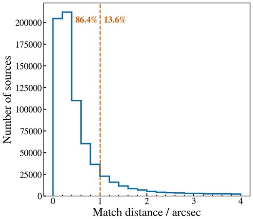
SDSS–WISE nearest counterpart cross-matching distance distribution. Numbers in orange indicate the fraction of sources in the accepted (left) and rejected (right) sections.
The initial set was based on the wise_xmatch catalogue, with every spectral and photometric match joined (where one existed). The total number of objects in this table is 495,003,196.6 From these, we selected sources using the following criteria:
W1 − W2 ≥ 0.8: This colour threshold has been shown by Stern et al. (2012) to be an efficient AGN selection criterion, yielding AGN samples with very high (∼95 per cent) reliability and good (∼80 per cent) completeness at high X-ray luminosities. AGNs are expected to heat dust to temperatures of several hundred degrees K, approaching sublimation, resulting in an SED peaking at a few microns and producing a red W1 − W2 colour. Whereas the colour cut alone can be contaminated by cool brown dwarfs, dust-reddened stars and star-forming galaxies (e.g. Stern et al. 2012; Yan et al. 2013; Hainline et al. 2014; Assef et al. 2018), our additional luminosity selection of only the most powerful sources is expected to weed out most such contaminants, preferentially selecting AGN alone (see step vi). We will return to this point in Section 6.
WISE–SDSS cross-match distance – required to be <1 arcsec as discussed above.
Reliable redshift:
z_ERR/z ≤ 0.01 – a fractional error of 1 per cent or less on the redshift, indicating an accurate value. This criterion was introduced because a good zWarning flag does not necessarily imply a robust redshift measurement. Note that, the median fractional z uncertainty in our final sample is 0.000 16, i.e. much smaller than the adopted threshold of 1 per cent which is designed to weed out the most obvious unreliable sources.
zWarning flag (SDSS) = 0, indicating high confidence in the redshift. Possible causes for a warning flag include poor or inconclusive fits, insufficient wavelength coverage, or problems with the instrumentation.
Redshift limit: 0 < z ≤ 0.83 (for SDSS spectroscopy) or 0 < z ≤ 1.065 (for BOSS spectroscopy) – this ensures that all spectra cover the redshifted [O iii]λ5007 line. For SDSS, this is identical to the redshift cut adopted by Reyes et al. (2008) for selecting [O iii]–luminous Type 2 quasars, thus allowing us to contrast this class of objects with our targets. We additionally include spectra from newer survey programmes, and as these use a wider wavelength range spectrometer, we can include some further objects.
ReliableWISEdata:
WISEcc_flags = ‘0000’. The four zeroes refer to the four WISE bands and indicate that the WISE data are not affected by any known artefacts that can cause confusion or contamination in any of the bands.
WISEW?ph_qual ≠ ‘U’ AND W?ph_qual ≠ ‘X’ AND W?ph_qual ≠ ‘Z’. This ensures a detection, reliable photometry, and measurable uncertainty in all WISE bands (with a signal:noise always above 2 and in the majority of sources above 3), allowing a robust measurement of the MIR source monochromatic fluxes (see the next point) as well as MIR SEDs.
IR luminosity:L12|$\, \ge 3\, \times \, 10^{44}$| erg s−1, where L12 is the k-corrected monochromatic 12 μm luminosity (λLλ), computed by simple linear interpolation between log(λLλ(W3)) and log(λLλ(W4)) to rest-frame. For the MIR versus X-ray relation of Gandhi et al. (2009), this L12 corresponds to an intrinsic 2–10 keV X-ray luminosity of ≥1044 erg s−1, widely adopted as the threshold for selection of sources with quasar X-ray luminosities (e.g. Gandhi et al. 2004; Brusa et al. 2009; Mainieri et al. 2011). Furthermore, the WISE extragalactic source population above this 12 μm luminosity threshold (corresponding to ≈ 1011 L⊙) comprises AGN almost exclusively (Donoso et al. 2012).
SDSS classification:CLASS = ‘GALAXY’ and SUBCLASS = ‘’–the CLASS selection removes sources with detected emission lines characteristic of QSOs (stars already having been culled by the redshift criteria). The SUBCLASS selection further removes sources with emission lines characteristic of Seyfert and LINERs, as well as star-forming and starburst systems.7
Best available spectrum:SciencePrimary=1. This indicates that the spectra are considered by SDSS to be the best available for each object.
No significant detection of [O iii]λ5007. The emissionLinesPort table contains detailed flux fitting of a large number of SDSS spectra, but has the disadvantage of not having been applied to many newer spectra. In order to include the maximum number of possible spectra, we measured the significance of the [O iii]λ5007 line flux directly, similarly to the method used to fit [O iii] lines when selecting for QSO2s (Reyes et al. 2008): Gaussian curves were fit to rest-frame positions of [O iii]λ5007 in the spectral data from SDSS. The outcome of this trial was that a subset of the objects had no apparent [O iii] emission line, and therefore these will comprise the final sample. A more detailed explanation of this trial is presented in Appendix B1.
Continuum SNR limit: Estimate of SNR in the direct region around where an [O iii] line would be detected. This is to remove any objects where the noise in the region of interest is overwhelming the measurement, leading to artificially high upper limits for the line flux. A more detailed explanation of this trial is presented in Appendix B3.
Visual inspection of sources: Automatic classification is not perfect, and a number of sources with e.g. obviously wrong redshift, classification, or visible emission lines were rejected in this final step.
An overview of the selection steps can be seen in Table 2.
Basic information about the 47 OQQs that passed the selection tests. A machine readable table can be found online. Column details: (1) short object name; (2),(3) sky position; (4) redshift; (5) rest frame 12 μm luminosity interpolated from W3 and W4 luminosities; (6) rest frame 5100 Å luminosity; (7) 4000 Å break; (8), (9) [O iii], H |$\alpha$| luminosity upper limits in units of L⊙; (10), (11) Minimum AV derived from different emission line luminosities; (12), (13) NH, derived from AV.
| Name (1) | RA (J2000) (2) | Dec. (J2000) (3) | z (4) | log L12 erg s−1 (5) | log L5100 erg s−1 (6) | D4000 (7) | [O iii]λ5007 L⊙ (8) | H |$\alpha$| λ6562 L⊙ (9) | AV ([O iii] derived) (10) | AV (H |$\alpha$| derived) (11) | log NH (cm−2) ([O iii] derived) (12) | log NH (cm−2) (H |$\alpha$| derived) (13) |
|---|---|---|---|---|---|---|---|---|---|---|---|---|
| OQQ J0002−0025 | 0.592 | −0.432 | 0.371 | 44.81 ± 0.02 | 44.00 ± 0.04 | 1.32 ± 0.21 | <6.69 | 8.15 | 5.87 | – | 22.91 | – |
| OQQ J0008+3144 | 2.226 | 31.749 | 0.600 | 44.71 ± 0.10 | 44.03 ± 0.08 | 1.71 ± 0.41 | – | – | – | – | – | – |
| OQQ J0021+3515 | 5.362 | 35.264 | 0.618 | 45.27 ± 0.03 | 44.00 ± 0.08 | 1.51 ± 0.27 | <6.26 | – | 8.15 | – | 23.05 | – |
| OQQ J0059+2502 | 14.757 | 25.049 | 0.802 | 45.02 ± 0.17 | 44.21 ± 0.11 | 1.22 ± 0.21 | <6.00 | – | 8.14 | – | 23.05 | – |
| OQQ J0101+0731 | 15.309 | 7.518 | 0.563 | 44.68 ± 0.14 | 44.40 ± 0.09 | 1.36 ± 0.14 | <7.20 | 7.98 | 4.24 | – | 22.77 | – |
| OQQ J0103−0349 | 15.792 | −3.830 | 0.507 | 44.52 ± 0.11 | 43.69 ± 0.11 | 1.28 ± 0.28 | <6.67 | 8.06 | 5.17 | – | 22.85 | – |
| OQQ J0109+0103 | 17.379 | 1.063 | 0.784 | 45.24 ± 0.13 | 44.47 ± 0.05 | 1.36 ± 0.08 | <6.26 | – | 8.06 | – | 23.05 | – |
| OQQ J0114+2002 | 18.622 | 20.047 | 0.589 | 44.61 ± 0.14 | 44.13 ± 0.08 | 1.59 ± 0.25 | <4.74 | – | 10.22 | – | 23.15 | – |
| OQQ J0141+1050 | 25.294 | 10.835 | 0.580 | 44.65 ± 0.11 | 44.01 ± 0.09 | 1.52 ± 0.29 | <6.78 | – | 5.21 | – | 22.86 | – |
| OQQ J0143+0151 | 25.844 | 1.859 | 0.334 | 44.72 ± 0.02 | 43.54 ± 0.05 | 1.42 ± 0.13 | <6.08 | <6.61 | 7.16 | 5.32 | 22.99 | 23.01 |
| OQQ J0149+3232 | 27.464 | 32.547 | 0.543 | 45.15 ± 0.02 | 44.10 ± 0.09 | 1.53 ± 0.97 | <6.78 | <7.80 | 6.53 | 3.63 | 22.95 | 22.84 |
| OQQ J0151+2540 | 27.929 | 25.671 | 0.661 | 45.07 ± 0.07 | 44.13 ± 0.17 | 1.25 ± 0.13 | <5.95 | – | 8.39 | – | 23.06 | – |
| OQQ J0231−0351 | 37.944 | −3.859 | 0.450 | 44.51 ± 0.05 | 43.74 ± 0.09 | 1.41 ± 0.26 | – | <7.18 | – | 3.28 | – | 22.80 |
| OQQ J0231+0038 | 37.990 | 0.648 | 0.488 | 45.06 ± 0.03 | 44.14 ± 0.03 | 1.51 ± 0.11 | <6.62 | 7.61 | 6.69 | – | 22.96 | – |
| OQQ J0237+0448 | 39.323 | 4.812 | 0.647 | 44.94 ± 0.08 | 44.07 ± 0.26 | 1.49 ± 0.18 | <6.81 | – | 5.90 | – | 22.91 | – |
| OQQ J0745+4301 | 116.493 | 43.021 | 0.517 | 44.74 ± 0.08 | 43.83 ± 0.08 | 1.82 ± 0.52 | <6.25 | 7.16 | 6.77 | – | 22.97 | – |
| OQQ J0751+4028 | 117.913 | 40.470 | 0.587 | 45.12 ± 0.05 | 44.09 ± 0.06 | 1.71 ± 0.22 | <6.85 | – | 6.28 | – | 22.94 | – |
| OQQ J0853+4533 | 133.324 | 45.554 | 0.776 | 45.89 ± 0.03 | 44.30 ± 0.09 | 1.21 ± 0.16 | <7.66 | – | 6.27 | – | 22.94 | – |
| OQQ J0911+2949 | 137.964 | 29.825 | 0.446 | 44.58 ± 0.06 | 44.36 ± 0.06 | 1.12 | <7.07 | 7.71 | 4.32 | – | 22.78 | – |
| OQQ J0926+6347 | 141.639 | 63.795 | 0.556 | 45.41 ± 0.02 | 44.32 ± 0.04 | 1.26 ± 0.09 | <6.77 | 7.58 | 7.24 | – | 23.00 | – |
| OQQ J0929+3253 | 142.306 | 32.896 | 0.781 | 45.05 ± 0.15 | 44.33 ± 0.06 | 1.58 ± 0.21 | <7.47 | – | 4.55 | – | 22.80 | – |
| OQQ J1015+2638 | 153.802 | 26.643 | 0.478 | 44.52 ± 0.10 | 43.88 ± 0.08 | 1.49 ± 0.25 | <6.74 | 7.49 | 4.99 | – | 22.84 | – |
| OQQ J1024+0210 | 156.191 | 2.170 | 0.549 | 44.59 ± 0.13 | 43.85 ± 0.09 | 1.77 ± 0.45 | <6.91 | <7.72 | 4.75 | 2.17 | 22.82 | 22.62 |
| OQQ J1051+1857 | 162.751 | 18.963 | 0.617 | 45.66 ± 0.02 | 44.06 ± 0.09 | 1.18 ± 0.23 | <7.17 | – | 6.90 | – | 22.98 | – |
| OQQ J1051+3241 | 162.794 | 32.699 | 0.932 | 45.94 ± 0.03 | 44.54 ± 0.17 | 1.11 ± 0.08 | <7.77 | – | 6.12 | – | 22.93 | – |
| OQQ J1116+4938 | 169.074 | 49.637 | 0.561 | 44.83 ± 0.06 | 44.12 ± 0.14 | 1.85 ± 0.42 | <6.95 | <7.60 | 5.28 | 3.19 | 22.86 | 22.79 |
| OQQ J1130+1353 | 172.614 | 13.894 | 0.635 | 44.93 ± 0.07 | 44.41 ± 0.05 | 1.04 ± 0.06 | <6.60 | – | 6.41 | – | 22.95 | – |
| OQQ J1156+3913 | 179.031 | 39.232 | 0.501 | 44.54 ± 0.09 | 43.81 ± 0.10 | 1.56 ± 0.39 | <6.09 | <7.09 | 6.66 | 3.60 | 22.96 | 22.84 |
| OQQ J1208+1159 | 182.155 | 11.994 | 0.369 | 44.77 ± 0.03 | 44.54 ± 0.03 | 1.08 ± 0.04 | <6.98 | <7.06 | 5.03 | 4.35 | 22.84 | 22.92 |
| OQQ J1242+5124 | 190.621 | 51.400 | 0.524 | 44.59 ± 0.10 | 43.99 ± 0.07 | 1.39 ± 0.19 | <6.86 | 7.26 | 4.86 | – | 22.83 | – |
| OQQ J1306+4028 | 196.613 | 40.472 | 0.582 | 45.38 ± 0.02 | 44.07 ± 0.13 | 1.44 ± 0.27 | <7.18 | – | 6.14 | – | 22.93 | – |
| OQQ J1320+5816 | 200.131 | 58.278 | 0.714 | 44.99 ± 0.08 | 44.17 ± 0.09 | 1.46 ± 0.18 | <6.90 | – | 5.79 | – | 22.90 | – |
| OQQ J1346+4639 | 206.582 | 46.654 | 0.522 | 44.59 ± 0.06 | 43.78 ± 0.15 | 1.73 ± 0.60 | <7.01 | 7.58 | 4.50 | – | 22.79 | – |
| OQQ J1412+1750 | 213.181 | 17.849 | 0.444 | 44.64 ± 0.04 | 43.88 ± 0.08 | 1.85 | <4.42 | – | 11.09 | – | 23.18 | – |
| OQQ J1417+1247 | 214.286 | 12.794 | 0.608 | 44.88 ± 0.07 | 44.15 ± 0.11 | 1.30 ± 0.18 | <7.02 | – | 5.24 | – | 22.86 | – |
| OQQ J1443+3955 | 220.869 | 39.929 | 0.817 | 44.90 ± 0.16 | 44.30 ± 0.09 | 1.11 ± 0.11 | <7.20 | – | 4.83 | – | 22.82 | – |
| OQQ J1454+1440 | 223.732 | 14.673 | 0.577 | 45.63 ± 0.02 | 44.15 ± 0.05 | 1.31 ± 0.14 | <6.93 | – | 7.42 | – | 23.01 | – |
| OQQ J1507+5932 | 226.885 | 59.550 | 0.620 | 44.90 ± 0.06 | 43.99 ± 0.09 | 1.34 ± 0.52 | <6.88 | – | 5.65 | – | 22.89 | – |
| OQQ J1526+5603 | 231.723 | 56.066 | 0.495 | 44.52 ± 0.06 | 43.98 ± 0.09 | 1.42 ± 0.22 | <5.01 | – | 9.30 | – | 23.11 | – |
| OQQ J1538+2911 | 234.691 | 29.193 | 0.477 | 44.58 ± 0.05 | 43.84 ± 0.12 | 1.66 ± 0.37 | – | <7.03 | – | 3.86 | – | 22.87 |
| OQQ J1540+4640 | 235.193 | 46.667 | 0.573 | 44.98 ± 0.03 | 43.99 ± 0.09 | 1.33 ± 0.22 | <6.97 | <8.16 | 5.61 | 2.22 | 22.89 | 22.63 |
| OQQ J1611+2247 | 242.864 | 22.787 | 0.809 | 44.98 ± 0.20 | 44.38 ± 0.11 | 1.18 ± 0.14 | <7.33 | – | 4.71 | – | 22.81 | – |
| OQQ J1611+2115 | 242.985 | 21.266 | 0.654 | 45.16 ± 0.05 | 44.07 ± 0.97 | 1.19 ± 0.10 | <7.32 | – | 5.22 | – | 22.86 | – |
| OQQ J1626+5049 | 246.532 | 50.817 | 0.522 | 44.57 ± 0.05 | 43.48 ± 0.25 | 1.35 ± 0.37 | <5.77 | <6.87 | 7.55 | 4.24 | 23.02 | 22.91 |
| OQQ J1629+4303 | 247.271 | 43.058 | 0.644 | 44.99 ± 0.07 | 44.31 ± 0.09 | 1.22 ± 0.08 | – | – | – | – | – | – |
| OQQ J2209+3044 | 332.427 | 30.734 | 0.482 | 44.68 ± 0.06 | 43.87 ± 0.06 | 1.58 ± 0.26 | <6.51 | 7.46 | 5.99 | – | 22.92 | – |
| OQQ J2229+2351 | 337.440 | 23.853 | 0.427 | 44.64 ± 0.04 | 44.00 ± 0.10 | 1.57 | <6.49 | 7.72 | 5.93 | – | 22.91 | – |
Process of cutting down objects. A full description of the steps is available in Section 3.
| Criteria | Number | Percentage | |
|---|---|---|---|
| Step 0 | Full xmatch table | 495,003,196 | |
| Step 1 | W1 − W2 ≥ 0.8 | 391,049 | 100.0 % |
| Step 2 | xmatch < 1 arcsec | 356,665 | 91.21 % |
| Step 3 | Redshift error < 1 % | 352,522 | 90.15 % |
| Step 4 | No redshift warning | 335,256 | 85.73 % |
| Step 5 | z in range | 89,425 | 22.87 % |
| Step 6 | Reliable WISE data | 50,207 | 12.84 % |
| Step 7 | L12 ≥ 3 × 1044 erg s−1 | 36,642 | 9.37 % |
| Step 8 | Class = GALAXY | 2,033 | 0.520 % |
| Step 9 | Subclass = null | 1,175 | 0.300 % |
| Step 10 | Primary science spectra | 1,025 | 0.262 % |
| Step 11 | No [O iii] by fitting check | 125 | 0.032 % |
| Step 12 | Estimated SNR ≥ 2 | 86 | 0.022 % |
| Step 13 | Visual check | 47 | 0.012 % |
3.1 Sample contaminants
Although the selection steps are designed conservatively to produce a clean sample, we must consider the possibility of contaminant objects; i.e. sources that pass all the same criteria but are not predominantly AGN powered.
Blazars (as discussed further in Section 6.3.7) are highly luminous and are generally lacking strong emission lines. However, the shape of their optical spectrum is often very distinct, and any clear blazars were removed in step (xi).
Luminous dusty star-forming galaxies may reach luminosities comparable to the OQQ threshold in rare cases. To assess this probability, we compare with the catalogue produced by Chang et al. (2015), selecting non-quiescent galaxies (using the threshold from Carnall et al. 2023) and processing them through the OQQ MIR selection. We find that only ∼0.01 per cent would pass the colour and luminosity criteria. If we also include the SDSS spectroscopic requirement for a null classification based on emission lines, no sources remain. This is logical, as any star formation intense enough to produce MIR emission on this level is likely to show strong emission lines on a galactic scale. The amount and distribution of dust that would be required to reduce the fluxes of these lines to the low levels detected (or upper limits of non-detections) would be highly unrealistic.
Compact Obscured Nuclei (CONs) (as discussed further in Section 6.3.1) may represent a more likely class of contaminants, although still low probability overall. These sources contain a dense, IR-bright core that may be powered by compact star formation or an AGN, but are usually found in LIRGs, ULIRGs, and disturbed systems which typically show strong optical emission lines. CONs are currently thought to be rare, but both their intrinsic power source and true number counts are unknown. We should note that they would only be considered contaminants if they are powered by star-formation – if they contain a strong AGN and reside in quiescent galaxies they would be correctly included as OQQs.
3.2 Comparison population
As a comparative and complementary sample, we use a combination of
The SDSS-selected sample of Type 2 quasars from Reyes et al. (2008). These are sources that are high luminosity (Lbol > 1045 erg s−1), show a significant [O iii]λ5007 line, and are optically obscured (Reyes et al. 2008).
A later, but similar, sample from Yuan, Strauss & Zakamska (2016) selecting QSO2s from both SDSS and BOSS spectroscopy.
These objects provide a valuable counterpoint to our selection, which is also based on high luminosity, but with no detectable [O iii]λ5007 flux. We combine the two tables, removing any duplicates. A small minority of sources were selected by Yuan, Strauss & Zakamska (2016) as having the wrong redshift fit by SDSS, and their corrected redshift is used in the processing. These are flagged in the table. The same procedure as used for the OQQs is used to match these QSO2s with WISE and the same luminosity cuts as outlined in Section 3 are applied to the combined catalogue to produce the final comparison set. The sample includes only objects at z<1.06, the range where [O iii] can be detected in BOSS.
4 RESULTS
4.1 General sample properties
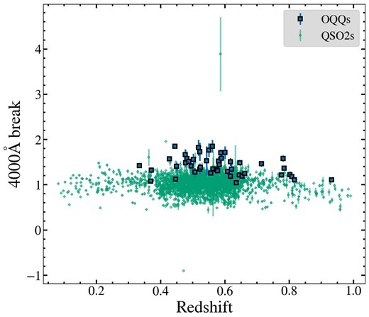
The number of sources that cumulatively pass all selections is 47. We refer to this sample as ‘Optically Quiescent Quasars’ or OQQs.8 Information on the final list is in Table 1. A sample of their spectra are in Fig. A1. The sources span a range in redshift of 0.33 ≤ z ≤ 0.94 (see Fig. 2). No sources show significant [O iii]λ5007 lines, by selection, but other low-level emission lines are present in several cases.
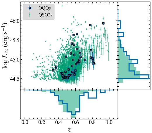
The 12 μm luminosity and redshift distribution of the OQQ sample and the QSO2s.
Fig.2 (main panel) shows the distribution across 12 μm luminosity and redshift for the OQQ sample and the QSO2 comparison set. Fig. 2 (bottom) shows the redshift distribution of both the OQQ sample and the QSO2 comparison sample, and Fig. 2 (right) shows the distribution with L12. The K–S statistic comparing the OQQ and QSO2 distributions is 0.073 for L12 and 0.209 for redshift, with p-values 0.874 for L12 and 0.007 for redshift. These results indicate that the samples are likely to come from populations with the same distribution in terms of luminosity, but with a different distribution in redshift. This is partly due to the combined selection of QSO2s from different studies, and the upgrade of the SDSS spectrometer – the original SDSS spectrometer would only allow measurements of [O iii] up to z ∼ 0.83, hence the jump in distribution at this point. This does not invalidate their use as counterpart objects, but may have implications for any detailed analysis of evolution over time.
4.2 Continuum properties
With regard to the infrared properties of the sources, the WISE colours are plotted in Fig. 3 on the canonical WISE colour–colour plane. The colours of all sources are consistent with being AGN-dominated in the MIR according to the Stern et al. (2012) colour cut, by selection. In addition, most of the sources also lie within the WISE AGN wedge proposed by Mateos et al. (2012).

Fig. 4 compares the WISE and SDSS luminosities of the sources. For each source, we plot the monochromatic 12 μm and |$5100 \,{{\mathring{\rm A}}}$| observed (i.e. not absorption-corrected) rest-frame luminosities (in λLλ).

Comparison of WISE, SDSS, and bolometric luminosities. OQQs are represented by outlined blue squares, and QSO2s by small green diamonds. Our luminosity threshold is shown by a horizontal dashed line. The dotted line represents where we would expect the points to lie if the IR and optical luminosities were equal.
The same figure also includes QSO2s: as already mentioned, QSO2s are likely to be a complementary sample to OQQs. All QSO2s with a WISE counterpart and MIR luminosity L12 > 3 × 1044 erg s−1 are included (as described in Section 3.2), mimicking our selection strategy, and resulting in a sample of 1990 QSO2s. The OQQ sample is reasonably well matched to the sample of QSO2s: at 5100 Å the average luminosity of the QSO2s is slightly dimmer, and the same (to a lesser extent) at 12 μm.
4.3 Emission line properties
Fig. 5 compares the 3σ limits on the [O iii] line luminosity with the observed MIR power. The dashed line denotes the relation |$L_{\rm [O\, {\scriptscriptstyle III}]}$|= 4 × 10⁻⁵ L12, which is the median ratio of the [O iii] limits to the 12 μm detections for the OQQs. The plot shows that our sources have a similar MIR luminosity distribution as QSO2s above the selection threshold of L12 > 3 × 1044 erg s−1. On the other hand, the |$L_{\rm [O\, {\scriptscriptstyle III}]}$| limits of OQQs clearly lie much below the corresponding typical line detections for QSO2s.
![A comparison of the 3σ upper limits on the [O iii]λ5007 luminosity of the OQQ (large outlined blue square markers) and of the QSO2 sample (small green diamond markers), and their respective 12 μm luminosities. The dashed line shows the slope of the relationship between QSO2 L12 and measured [O iii], scaled down by the average deficit.](https://oup.silverchair-cdn.com/oup/backfile/Content_public/Journal/mnras/527/4/10.1093_mnras_stad3964/1/m_stad3964fig5.jpeg?Expires=1749806887&Signature=CWYir9beQXNcKrTCcxcX3xPSvPqLij9YZuOAfYSRDn2D33w6JjfakIA1Y6~8PvTE5ksvx1VYzgBxrXvZIUZQqHw4UewOMgbL64kPzeQ4WIKf3EyNvk0IPbsNSG1Z3U0vfpRx9IytsslzNIeJuOXoUwjRNJiYRb5YqTBi~SDx38DPMXSZYg5DDBbDnA7CMPHMyQSxlmOKQ-FznuqI25o2nNj3xU15Mh85cMTnl--8y~0vkFoccZvduZ7hNoW9GTJTX~CLel23Xex4NQ14rwMwFV~wwLBzQ4m0epqm1E3Ts~rlKsQWnHQfcBZ894d3DBaYe52oqLVJewrPe~Q5n-skPA__&Key-Pair-Id=APKAIE5G5CRDK6RD3PGA)
A comparison of the 3σ upper limits on the [O iii]λ5007 luminosity of the OQQ (large outlined blue square markers) and of the QSO2 sample (small green diamond markers), and their respective 12 μm luminosities. The dashed line shows the slope of the relationship between QSO2 L12 and measured [O iii], scaled down by the average deficit.
In the following steps, we fit lines to the OQQ and QSO2 populations in order to estimate the reddening effect of the obscuring material on an average rather than individual source level. This line should not be taken as an indication of a relationship between the two properties – as we are only fitting upper limits it will be heavily effected by e.g. level of obscuration and/or intrinsic luminosity of the source. For this reason, we have not made any special considerations in the fitting method for the fact that these are upper limits.
A simple linear fit to the relation between |$L_{\rm [O\, {\scriptscriptstyle III}]}$| and L12 (in log space) for QSO2s gives us the equation
This fit is based upon the ordinary least squares bisector method of Isobe et al. (1990). There is significant scatter of 0.11 dex and a Spearman rank correlation coefficient of 0.40 indicates that the relation is not very strong. Nevertheless, this serves as a guide for comparison to OQQs.
The dotted line denotes an [O iii] deficit of ∼253 × from the above fit. This is the mean deficit of our OQQs relative to the expected intrinsic [O iii] luminosity if they are typical quasars similar to QSO2s. Since these are upper limits, this should not be considered a true fit to the data, but merely allows us to estimate the scale of obscuration present. The actual deficits could be much larger, and potentially show a different relationship to 12 μm luminosity. One can perform a similar comparison using the H |$\alpha$| emission line, as it is less affected by reddening. The result is shown in Fig. 6.
The corresponding relation for QSO2s is
QSO2 [O iii]λ5007 fluxes from the source papers (Reyes et al. 2008; Yuan, Strauss & Zakamska 2016) were used, but H |$\alpha$| λ6562 were drawn from the emissionLinesPort table. Since we are only using the QSO2 sample for comparison, we did not perform our own H |$\alpha$| line flux measurements. Above z ≈ 0.35, when redshifted H |$\alpha$| is shifted to |$\gtrsim$|9000 Å, the sky noise can often render lines difficult for the pipeline to measure correctly. Therefore, we restricted the QSO2 sample to below this redshift for extracting robust automated H |$\alpha$| fluxes. This results in few QSO2s for the above fit, all of which have a significant H |$\alpha$| detection without having been specifically selected on this line, as one would expect for a standard quasar spectrum. The scatter in this case is 0.10 dex with a Spearman rank correlation coefficient of 0.48.
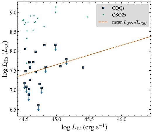
A comparison of the H |$\alpha$| λ6562 luminosity (or its upper limit – out of the sample of 62 OQQs, 17 have detected H |$\alpha$| emission lines), with OQQs (large blue square markers) and QSO2s (small green diamond markers), and their respective 12 μm luminosities (for those objects where Hαλ6562 is not redshifted out of the SDSS range). The dashed line shows the slope of the relationship between QSO2 L12 and measured Hα, reduced by the average deficit.
The OQQs have a median distribution (either a detection or a limit) consistent with an H |$\alpha$| deficit of ≈27. This is less than the deficit found from [O iii] partly because of the lower reddening affecting H |$\alpha$|, and partly because redshifted H |$\alpha$| typically lies in the reddest portions of the spectra with strong noise from sky emission lines resulting in less sensitive non-detection flux limits. Another possibility is that H |$\alpha$| has a larger fraction of its flux coming from star formation, while [O iii] is likely primarily from the AGN.
4.4 Spectral Energy Distribution (SED) fitting
We use agnfitter (Calistro Rivera et al. 2016) to fit the SEDs of a selection of OQQs and determine contributions to the observed emission from different components of the AGN/galaxy system. This method uses the multiwavelength data available to find the most likely weighted contributions to the overall SED, using Markov Chain Monte Carlo (MCMC) to fit from a large library of models. The most important parameter for our analysis is the contribution to the SED from the AGN obscuring material. We select the candidates with available long wavelength data (2MASS9, Herschel, in addition to all four WISE bands, present in all OQQs by selection), as this is key to constraining some components; this totals only 9 sources10. Fig. 7 presents the results from four OQQs that have reasonably well-constrained results. After experimenting with different MCMC lengths, we selected one sufficient to achieve an autocorrelation time indicating convergence for the OQQ AGN-heated dust component (see Foreman-Mackey et al. 2013 and Calistro Rivera et al. 2016 for details). Settings used were: 100 walkers; two burn in sets (10,000 steps each); set length 200,000.
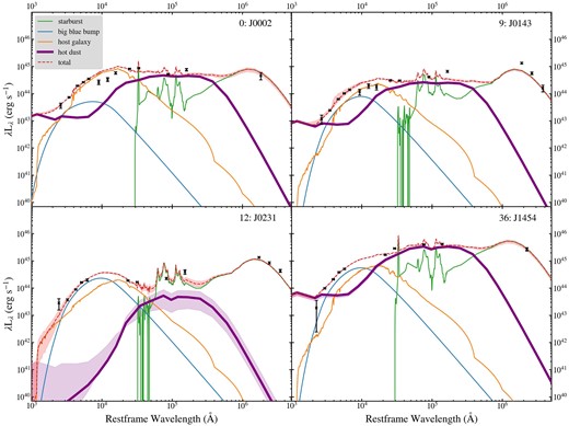
agnfitter results for four candidate OQQs with long wavelength IR data. The hot dust component – that most indicative of an AGN – is highlighted (thick purple line). Errors are shown for this component and the total only. Photometric bands used in this plot (in addition to SDSS ugriz and WISE W1-4) were as follows: OQQ J0002-0025 all 2MASS and 250 μm; OQQ J0143+0151 all 2MASS and the three Herschel bands stated in footnote 10; OQQ J0231-0351 three Herschel bands; OQQ J1454+1440 350 μm only.
In some cases, the hot dust component (e.g. the top two plots in Fig. 7) rises towards the blue end. This would not occur in a purely physical model component, but it is an empirical template based on combinations of AGN SEDs from Silva, Maiolino & Granato (2004), and the range of values these can take can be seen in Fig. 1 of Calistro Rivera et al. (2016) and Fig. 1 of Silva, Maiolino & Granato (2004); they are based on NH and assumed AGN type. As can be seen in these figures, the peak remains unchanged, varying only with normalization. With further data into the blue and near-UV, we may be able to take this as some indication that the OQQ in question is lightly obscured, or at least has some accretion disc emission visible, but currently degeneracy with ‘host galaxy’ emission (solid orange line) makes this conclusion premature. Nevertheless, while the general results should be used with caution, the key outcome is that a high normalization of the ‘hot dust’ component (see Fig. 7, thick purple line) is required to reproduce the MIR part of the OQQ SEDs regardless of the tail shape (i.e. the peak of the hot dust component at ∼6–20 μm in the rest frame). We conclude it is very likely each of these objects contains an AGN bright enough to heat its obscuring dust to produce this component. agnfitter makes two separate estimates of star formation rate (SFR) – one in the optical, and one in the FIR. The FIR SFR provides an estimate of potential obscured star formation, but we note that very few candidates have reliable data in that region, so we cannot make any conclusions about the whole OQQ population. This estimate (and that of stellar mass) is obtained from host galaxy template parameters (for more detail, see Calistro Rivera et al. 2016).
4.5 4000 Å break
The 4000 Å break (D4000 from this point on), an indicator of a significant population of old stars, was calculated as described in Balogh et al. (1999), as the ratio between red (4000–4100 Å) and blue (3850–3950 Å) continuum fluxes. These ranges are slightly more restrictive than in previous works (e.g. Hamilton 1985), as this was found to improve on the repeatability of D4000 between separate measurements, and shows less sensitivity to reddening. A large 4000 Å break could be indicative of significant host galaxy light dilution. The values are found in Table 1 and shown in Fig. 8: 44 out of 47 (94 per cent) objects have a significant D4000. The median value is 1.41 (including only the significant breaks, defined as >3 standard deviations above unity). The QSO2 sample found only 811/1988 (41 per cent) had a significant D4000.
|$4000 \,{{\mathring{\rm A}}}$| break data. Blue squares are the OQQs, with error bars shown for those with D4000 significantly greater than 1. Green diamond markers are the QSO2 comparison sample. The average D4000 is clearly higher for OQQs than QSOs, implying a difference in the host galaxy population. However, this may be a selection rather than intrinsic effect.
5 X-RAY OBSERVATIONS
In the absence of AGN spectroscopic signatures in the optical, X-ray observations arguably provide the best evidence for the presence of an AGN independent of the MIR signatures. We checked the heasarc archive.11 for pointed or serendipitous observations by X-ray satellites, and discovered several OQQs observed during targeted observations of other nearby objects. We also obtained joint XMM–Newton and NuSTAR (Harrison et al. 2013) data for our prototypical OQQ (see Section 6), and these results are discussed in Section 5.1. Details of a serendipitous observation with sufficient counts for fitting are presented in Section 5.2.
The XMM–Newton mission has one of the best combinations of effective area and angular resolution of current X-ray missions, and is therefore an ideal tool to help us analyse the X-ray properties of OQQs. Chandra, which has very low-background noise, can also be valuable in detecting dim sources. We also examine Swift– XRT data – this is generally less sensitive, but in cases where no XMM–Newton or Chandra data are available Swift-XRT can still be useful to place limits on the X-ray emission. For detected sources, we extracted source and background spectra using standard ftools tasks and recommended reduction steps for each instrument, and analysed the data using the xspec package (Arnaud 1996). We then assessed the false detection probability based on counts in the source region relative to counts in a background region, and this derived either estimated fluxes or upper limits for each target (see e.g. Lansbury et al. 2017). Figs 11 and 12 show the results of analysis of data from XMM–Newton, Chandra, and Swift -XRT for OQQ candidates with serendipitous observations – in total 11 separate OQQs (See Table D2). These are discussed further in Section 5.3.
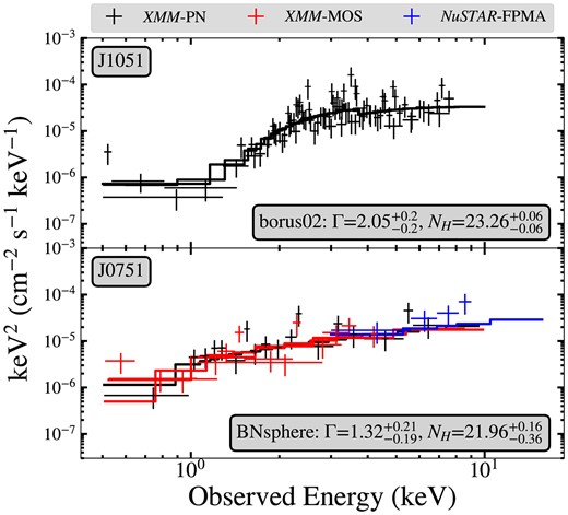
X-ray spectra of two OQQs. Top panel: OQQ J1051+3241, fitted with borus02; bottom panel OQQ J0751+4028, fitted with BNsphere. The sources have several differing properties (e.g. NH, intrinsic spectral shape) but have underluminous intrinsic luminosities (see Fig. 11).
The SDSS spectrum of OQQ J0751+4028 is shown in Fig. 10 (bottom spectrum), and (by selection) shows typical properties for an OQQ (compared to examples from the general sample in Fig. A1 and online). For more detail, see Greenwell et al. (2021).
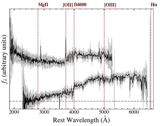
SDSS spectra of OQQ J1051+3241 and OQQ J0751+4028. J1051 shows a slight blue rise which may indicate that there is either some view of the accretion disc or recent star formation (see Appendix B2), whereas J0751 shows the continuum shape and lack of emission lines of typical OQQs.
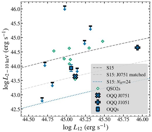
Observed 2–10 keV luminosities of the OQQs (blue markers), plotted against their 12 μm luminosities. OQQ J0751+4028 is shown as a large cross marker. For comparison, available QSO2 luminosities are shown as diamonds (see Table D1). We also show MIR predicted values for intrinsic luminosities (dark grey dashed line; Stern 2015). If this relationship is scaled to the luminosity of J0751 (pale grey dashed line; Greenwell et al. 2022), the other detected OQQs are more consistent with this expectation. Upper limits may be better explained by a Compton thick scenario: dotted blue line shows the obscuration of the S15 relation by Compton thick material.
![2–10 keV luminosities of the OQQs (blue markers), plotted against their [O iii] upper limit luminosities. OQQ J0751+4028 is shown as a large cross marker. For comparison, available QSO2 luminosities are shown as diamonds (see Table D1). We also show [O iii] predicted values for intrinsic luminosities (solid line; Lamastra et al. 2009).](https://oup.silverchair-cdn.com/oup/backfile/Content_public/Journal/mnras/527/4/10.1093_mnras_stad3964/1/m_stad3964fig12.jpeg?Expires=1749806887&Signature=aereVE2lx2h3sO7-l~jw-cS8MhCjE2CEt9vNjeXYtE6Sjvu5Xfrw24NTI7SmkevGR04Zj6t4UX504c5Yy9~-tf9Y-bO5vbEb2gd3D2nKZ-R51wrgxd0YzDe~OxZsNcGzWoJy26CXWl6mvwvvDLf3lpxuaGJrhBUd7uS3Xh33cHVkP1UqQHnL8Ed8WpEmb6c6WrSiwJsKy2o-YcJurl-Be1xdALSiv9eN3IUK2oomRCx1YsbjxhpkOWJ~Zx-BEW95ct~hOHP-Dex6hO-7V-eJAvkF2CNfDdgp0QSZEdxU0mJTxCu~6R3U9aeIEn6y5ESGzZtQJzgmjcVYQF362ln1LA__&Key-Pair-Id=APKAIE5G5CRDK6RD3PGA)
2–10 keV luminosities of the OQQs (blue markers), plotted against their [O iii] upper limit luminosities. OQQ J0751+4028 is shown as a large cross marker. For comparison, available QSO2 luminosities are shown as diamonds (see Table D1). We also show [O iii] predicted values for intrinsic luminosities (solid line; Lamastra et al. 2009).
5.1 X-ray observations of OQQ J0751+4028
We obtained targeted observations of our prototypical candidate with the aim of confirming its AGN nature and constraining its properties. Following standard procedures with xspec, we modelled the source, finding that it is under-luminous at 2–10 keV (compared to the IR-predicted intrinsic luminosity), and appears to be lightly obscured (NH∼1022 cm−2). This work is summarized here: for details of the observations and procedures, see Greenwell et al. (2022).
We fit several models, starting with an absorbed power law (cabs*zwabs*pow), moving on to more physically realistic models (mytorus; Murphy & Yaqoob 2009; BNsphere; Brightman & Nandra 2011) and finally a more complex model involving a lightly obscured leak in an otherwise Compton thick sphere of obscuration. Using Bayesian X-ray Analysis (BXA; Buchner et al. 2014), we can compare the results and determine the model most likely to have produced the data. We find that BNsphere is favoured – a spherical obscuration model that implies a ‘cocooned’ obscuring structure may be a plausible explanation for the X-ray appearance of OQQ J0751+4028. This result is shown in Fig. 9 (bottom panel).
Fig.11 shows OQQ J0751+4028 in context with the serendipitous observations and the empirical relationship between 12 μm and intrinsic 2–10 keV luminosity. The unobscured rest frame 2–10 keV luminosity is 4.39 × 1043 erg s−1, approximately a factor of 6 lower than expected given the 12 μm luminosity, but sufficient to categorically demonstrate the presence of an AGN. The photon index is harder than usual for an AGN (Γ = 1.32|$^{+0.21}_{-0.19}$|), and obscuration is approximately Compton-thin but present (log (NHcm−2) = 21.96|$^{+0.16}_{-0.36}$|). If Γ is fixed to a more usual AGN-like value of 1.9, the obscuration increased only slightly to log (NH/cm−2) = 22.3.
5.2 Serendipitous X-ray observations of OQQ J1051+3241
One serendipitous OQQ had sufficient XMM–Newton counts across two observations (0781410101 and 0781410201; both only observed the source with the PN detector) to be analysed further with xspec. We fit this source (OQQ J1051+3241) with several models, as was done with the targeted observations of OQQ J0751+4028 (see Section 5.1 and Greenwell et al. 2022). We find the best-fitting model to be borus02 (Baloković et al. 2018), at fixed angle of inclination assuming viewing through the torus (cos θ = 0.05). We do not find a significant Fe K α emission line, and allowing the angle of inclination to vary does not favour any angle strongly. This object is more obscured and has a higher Γ than J0751: log (NHcm−2) = 23.26 ± 0.06, Γ=2.05 ± 0.2 (see Fig. 9, top panel). For all sources (with the exception of our targeted observation; Section 5.1), we have assumed the same photon index as for this source, and used WebPIMMS12 to estimate the luminosity of each source, given the net counts (or upper limit) observed. We find that the detected OQQs are underluminous compared with expectations. If the non-detected OQQs are equally underluminous, they may still be detectable with sufficiently long observations.
The SDSS spectrum of OQQ J1051+3241 is shown in Fig. 10 (top spectrum). In this case it shows a slight rise towards the blue end, implying that this is not as strictly ‘typical’ of an OQQ as OQQ J0751+4028.
5.3 Discussion of X-ray results
Fig.11 shows the comparison between X-ray and 12 μm luminosity, including the predicted relationship between intrinsic X-ray and nuclear 12 μm luminosity from Asmus et al. (2015) and between X-ray and 6 μm luminosity (Stern 2015); for the latter, 6 μm luminosities were converted to 12 μm luminosities using a relationship derived from the QSO template of Hao et al. (2007). The OQQ X-ray luminosities are slightly lower than the relations would predict, but this may be due to the difference between observed and intrinsic IR luminosities – if the OQQs are heavily obscured (whether from the circum-nuclear material or larger scale obscuration), their intrinsic luminosities will be higher. OQQ IR luminosities refer to the total galaxy emission, not the nuclear emission alone, as with current data there is no reliable way to extract or convert this for individual objects. Fig. 11 shows where obscuration-reduced MIR-predicted X-ray luminosities (Asmus et al. 2015; Stern 2015) would fall. This would imply that most OQQs lie somewhere between Compton thick and unobscured. However, if they are intrinsically similar to OQQ J0751+4028 (Greenwell et al. 2022), the obscuration depth is low for an obscured AGN (NH∼1022 cm−2), and thus the intrinsic values for the OQQs may be only slightly higher. Fig. 12 shows the relationship between [O iii] and X-ray luminosity found by Lamastra et al. (2009), with the QSO2s falling where expected. Upper limits on [O iii] luminosity place the OQQs significantly below expectations, reinforcing the disconnect between observed [O iii] and intrinsic properties.
6 DISCUSSION
The combination of WISE all-sky MIR photometry and SDSS optical spectroscopy have enabled us to identify an interesting class of sources showing all the characteristics of luminous AGN in the MIR (based upon their colours and luminosities) but no obvious signatures of the corresponding AGN activity in the optical.
Multiple physical scenarios can explain these observations, principally based on whether the optical AGN signatures are obscured, or intrinsically absent. In the former, we can consider the OQQ in terms of the spatial scale of its obscuration. As opposed to the putative donut shape envisaged by the zeroth order AGN unified torus scheme, full or near full sky covering by dusty ‘cocoons’ could easily explain the optical absence of emission signatures by not allowing an extended NLR to form or be ionized in the first place. Such cocoons would still reprocess the intrinsic AGN emission to the MIR, and the high WISE luminosities (along with bright hot dust component, where SED fitting is available) of these sources strongly suggest that the underlying power sources are luminous quasars, as does the MIR comparison with SDSS-selected QSO2s. For the latter scenario, AGN emission lines are not currently produced by the OQQ. We can envisage this as a ‘young’ AGN – recently switched on, with the AGN radiation not yet ionizing the NLR, and consequently no narrow emission lines. It is still likely that this is an obscured AGN, i.e. that it is being viewed through a dusty torus, which would hide any broad emission lines (produced closer to the supermassive black hole (SMBH), and therefore earlier in the switching on process). As in the ‘cocooned’ picture, reprocessed intrinsic emission can still produce the observed IR properties.
We previously identified a prototypical example of this class, described in Greenwell et al. (2021) and Greenwell et al. (2022). We found that it indicated a new subclass of AGN that does not easily fit into current models:
The spectral shape of the optical continuum is that of a typical galaxy, including showing a strong 4000 Å break.
Strong upper limits on emission lines that may indicate the presence of an AGN – there is no [O iii] by selection. Others may be present at a very low level.
The WISE IR colours are firmly within the AGN wedge (Mateos et al. 2012), a stricter criterion than that required for the main sample selection.
The 12 μm luminosity is very high, consistent with the quasar regime: there is a high chance of a hidden AGN being present, and it is not likely that this comes from a different mechanism.
X-ray luminosity is luminous enough to clearly indicate the presence of an AGN, but underluminous compared to expectations from 12 μm luminosity (see 5.1).
An upper limit on radio flux is available from FIRST (Becker, White & Helfand 1995): <0.695 mJy beam−1.
6.1 Optical reddening
(Non)-detection of emission lines can be used to place constraints on the optical depth of the theoretical cocoons, if present (see Section 6.2.2). We assume that the QSO2s have low extinction to their NLRs (an approximation), and that therefore the relationship between 12 μm and [O iii] luminosity (H |$\alpha$| luminosity) (equations 1 and 2 above) can be used to predict the approximate intrinsic flux of a cocooned source at the same 12 μm luminosity (assuming that all OQQs had [O iii] signals at the upper limit of detection. The extinction AV can be calculated using this predicted flux, the actual measured flux, and the standard Milky Way extinction law of Cardelli, Clayton & Mathis (1989) with an RV = 3.1. The resultant values of the extinction AV as derived from the two lines are listed in Table 1. Since QSO2s are also likely to suffer mild NLR extinction (Reyes et al. 2008), these should be regarded as lower limits on the true AV. The AV limits measured from the [O iii] non-detections range over 3.4–10.5 mag, with a median value of 4.69.
What would be the corresponding column density of gas for this extinction? A factor of 100 deficit in [O iii] does not need extreme columns. Our median extinction AV = 4.69 mag is equivalent to a neutral gas column of |$N_{\rm H}^{\perp }$| ∼ 7 × 1022 cm−2 along the galaxy axis, assuming the gas–to–dust ratios found in AGN environments by Maiolino et al. (2001). The parameter |$N_{\rm H}^{\perp }$| is used to denote the fact that these gas columns are relevant for the NLR, which is likely to probe angles out of the direct l.o.s., thus making the distinction from the |$N_{\rm H}^{\rm los}$| measured from X-rays in the previous section. Further speculations on the gas columns or spatial distributions with only two detected objects would be premature. The |$N_{\rm H}^{\perp }$| values are lower limits inferred from the limits on the optical extinction, so it is unexpected that the |$N_{\rm H}^{\rm los}$| would be lower.
Fig. 13 shows the |$N_{\rm H}^{\perp }$| values inferred from [O iii] extinction. In a small number of cases, this can also be calculated using H |$\alpha$| (see Table 1). Where a H |$\alpha$|-inferred value is available, the predicted NH is consistently lower, and as some of these emission lines are measured rather than upper limits, are likely to be closer to the true value.
![Inferred $N_{\rm H}^{\perp }$ values from [O iii] (i.e. obscuring the NLR, distinct from the $N_{\rm H}^{\rm los}$ related to X-ray obscuration).](https://oup.silverchair-cdn.com/oup/backfile/Content_public/Journal/mnras/527/4/10.1093_mnras_stad3964/1/m_stad3964fig13.jpeg?Expires=1749806887&Signature=s0KQGkPUVICQfYqtvp5kJwqJjFxV4EDEh23~kGiOZ2vVPPgfMTNQ6Kwv0cCqUf3RCCk2Eh~CeJbq~WP1t1E5sXC3XzJ514thPjcvSx9Skvvo9Oxo3qonBreb~4MNKWZUNyWel7wW~lc9GJGlnUtfjXGMQrd3sOJP1HT1HLaTQzNJqxen2YWaS9V-2ZtBXHEsF0AdGKN6Mjir8tG66QUvZoEEgTsImEH6vHVzSNntzXixzl~T0LXkgm263D1gfQAa57bmcaVlRZy4eLgC3fk1VqaNKP2Ma0EB06L4UKqWjcBXAi5IZesEuruFZoZn~Ew86zo8bk03iPxIu3zsLuyj7g__&Key-Pair-Id=APKAIE5G5CRDK6RD3PGA)
Inferred |$N_{\rm H}^{\perp }$| values from [O iii] (i.e. obscuring the NLR, distinct from the |$N_{\rm H}^{\rm los}$| related to X-ray obscuration).
6.2 Intrinsic nature
It is difficult at this stage to make definitive statements about the true intrinsic nature of OQQs, but we can speculate on some likely possibilities. A schematic comparison between QSO2s and theories on OQQs can be found in Fig. 14. In Section 6.3, we discuss how these theories might relate OQQs to various other object classes.
![Schematic showing (left) a typical QSO2, producing a spectrum with strong [O iii], (middle) an OQQ that is intrinsically ‘young’, with no [O iii] produced, and (right) a ‘cocooned’ OQQ, producing typical [O iii] emission that is obscured by a larger region of material, with the observer positioned to one side of the diagram. Inset boxes show a zoom in on the [O iii] region of the spectrum – a strong line in the QSO2, but not detected in the two OQQs. Components are as follows: black central circle for SMBH, blue accretion disc, dark brown standard torus, green trapeziums for ionized gas, lighter brown annulus for ‘cocoon’. Composition of dust/obscuring material may be different across various parts of these structures.](https://oup.silverchair-cdn.com/oup/backfile/Content_public/Journal/mnras/527/4/10.1093_mnras_stad3964/1/m_stad3964fig14.jpeg?Expires=1749806887&Signature=eX7YNRxcyvWAM6af4vao5emamFh4cfTUGmpCLF-N~yp11O-iKhzbmbhj8JbQy8TaY8P8DCAxkUJNouCfsxOnt6AUDNROE-1DpDAVqMpIARkz~XHYiZSlPXRemt0UCEjk8Rn1i3Y8L3~E8VWi2Byr5592KcWLdSPGWhy~hzITAfO0xf0P0H5lOjqHEqybdKMp7U1Sm0vMCRulIOxBHyfkERvAQgiRC8GXkGtNlqr-hB0LbHPkE3FciZKl40ulUkG8cVQ2hvXaeQoam6mRviFEmyKlGNJa0pk3lK90T5b9nmE1I6QGlSThIR8mc2filoj0-OkxwEp0eMMCqDvZtcUgYg__&Key-Pair-Id=APKAIE5G5CRDK6RD3PGA)
Schematic showing (left) a typical QSO2, producing a spectrum with strong [O iii], (middle) an OQQ that is intrinsically ‘young’, with no [O iii] produced, and (right) a ‘cocooned’ OQQ, producing typical [O iii] emission that is obscured by a larger region of material, with the observer positioned to one side of the diagram. Inset boxes show a zoom in on the [O iii] region of the spectrum – a strong line in the QSO2, but not detected in the two OQQs. Components are as follows: black central circle for SMBH, blue accretion disc, dark brown standard torus, green trapeziums for ionized gas, lighter brown annulus for ‘cocoon’. Composition of dust/obscuring material may be different across various parts of these structures.
6.2.1 Young AGN
A form of changing look AGN (e.g. Yang et al. 2018), objects belonging to this class have been recently activated such that they heat the torus to produce strong IR signals. However, radiation has not extended far enough to ionize the outer NLR, where the [O iii] we normally see in QSO2s is produced (middle diagram in Fig. 14). For example, Gezari et al. (2017) present an example of a ‘switching-on’ AGN that goes from the appearance of a LINER to a Type-I quasar over less than 1 year. No [O iii] is found in the ‘before’ or ‘after’ spectra, due to [O iii] following longer term AGN activity than other narrow emission lines, such as H |$\alpha$|, which increase strongly. If OQQs are an obscured analogue to this object, it follows that we are unable to detect other emission lines. They must be observed through the torus, as otherwise we would still observe the broad emission lines produced closer in. If this is the case, and we expect broad emission lines to be present, then detection of these in spectral ranges less subject to obscuration could provide evidence for this explanation (e.g. NIR measurements; Onori et al. 2017a). An analogous and opposite population would be those described in Saade et al. (2022) which have low X-ray luminosity when compared with their strong [O iii] emission, with one possible explanation being a ‘switching-off’ AGN. They find an example with NLR and nuclear MIR emission but low X-ray luminosity and conclude that this object has recently become inactive. Discovery of this object among their relatively small parent sample implies that AGN caught ‘mid-change’ may not be extremely rare; we might expect ‘switching-on’ AGN to be found in similar numbers.
6.2.2 ‘Cocooned’ AGN
This type of OQQ would be more mature than a young AGN, and has similar intrinsic features to a QSO2, but with a ‘cocoon’ of obscuring material preventing either observation of the NLR (right diagram in Fig. 14), or its formation entirely. This ‘cocoon’ is likely to be unstable, and as such these objects may only have a short lifetime, suggested by the small number counts found when compared to QSO2s.
At z ≈ 0.5 for most of our sample, a physical size of 1 kpc corresponds to an angular size of 0.16 ″, so any circumnuclear dust on sub-kpc scales would certainly be unresolved in most ground-based imaging. If the cocoon is comparable in radius to the dust sublimation radius, it may be even smaller – pc-scale – and thus unresolvable even with instruments such as ALMA. However, high resolution imaging might be expected to show very late stage mergers or other disturbances in the centres of these galaxies, as the source of the ‘cocoon’, despite the ‘cocoon’ itself being unobservable. We searched public archives such as MAST13 and the Virtual Observatory14 for any high angular resolution imaging of our targets, but these fields have not been observed with HST, nor with any other large ground-based observatory. In SDSS imaging (as well as WISE), the targets do not show any special characteristics, preferred morphologies or orientations, nor obvious disturbances. This appears to support small physical scales for any putative dust cocoons in our sample. However, it must be cautioned that SDSS imaging is seeing-limited and not very deep, so for fainter sources, signatures of interaction may be missed.
6.3 Comparison with other object classes
Although the idea of optically quiescent AGN is not new, there are no close counterparts of our selected sample, at least in the local Universe. In this section, we briefly compare and contrast other related samples with the OQQs.
6.3.1 ULIRGs
Our selected targets have total MIR powers within or close to the ULIRG regime. ULIRGs tend to be hosted in chaotic appearing systems, with little clear structure and sometimes lack important optical emission lines, but are not usually completely devoid of strong emission signatures. For example, Mrk 231 has much stronger H |$\alpha$| than [O iii]λ5007 emission (Lacy et al. 1982; Malkan et al. 2017). Several local ULIRGs are also considered as being ‘buried’ AGN obscured along all lines of sight (e.g. Imanishi, Dudley & Maloney 2001; Oyabu et al. 2011). These are typically associated with sources that have LINER-like optical spectra with clear emission lines (Imanishi et al. 2007).
As discussed in Section 4.3, 15 of the 28 sources for which redshifted H |$\alpha$| lies within the SDSS spectral range show significant H |$\alpha$| emission. These sources may be similar to ULIRGs such as Mrk 231, though the comparison with SDSS-selected QSO2s implies that H |$\alpha$| also suffers some extinction, as already discussed. The remaining objects clearly differ from local ULIRGs in their lack of H |$\alpha$|. This may be explained by correspondingly higher NLR dust covering factors in the ‘cocooned AGN’ scenario. It could also be a sign that the dust distribution in the galaxy is less centrally located, additionally obscuring H |$\alpha$| from sources other than AGN ionization.
Compact Obscured Nuclei (CONs) are found in LIRGs and ULIRGs (e.g. Falstad et al. 2021). They are dense, IR bright cores found at the centre of an optically normal galaxy. The strength of the IR emission indicates a heavily obscured nucleus, with either a compact starburst or AGN powering the luminosity. One intensively studied example is NGC 4418 (Costagliola et al. 2013; Asmus et al. 2014; Ohyama et al. 2019), which appears optically as an Sa type galaxy, and is part of an interacting pair. Extreme visual obscuration is demonstrated by a very deep silicate absorption feature in the MIR, and high resolution imagery shows a small, optically thick core. Ohyama et al. (2019) find that a dusty wind and compact starburst activity are present in the core, but that an additional energy source in the core is still required to explain the observations; it is still currently unknown whether this is an AGN or an extremely compact starburst. In a study with NuSTAR, Ricci et al. (2021) do not detect it and find that a SF model fits the data better, implying either no AGN or extremely thick column densities.
CONs are not very well understood, and there are not many examples. Falstad et al. (2021) search LIRGs and ULIRGs for compact sources of HCN vibrational emission, which are only found in extreme environments. They find that 40 per cent of ULIRGs and 20 per cent of LIRGs contain a CON, noting that their sample size is not large, and that the selection in the FIR does introduce some biases. This indicates that CONs are relatively common in (U)LIRGs; however, (U)LIRGs themselves are not extremely common.
OQQs are also bright in the IR, but are at larger distances than these prototypical CONs tend to be. Without high resolution imaging, it is impossible to definitively say whether the OQQs are equally compact. Unlike NGC 4418, OQQs appear to be small red galaxies with no obvious signs of interaction.
6.3.2 Weak line and lineless quasars
At higher redshifts, several studies have been made of ‘Weak Line Quasars’ (WLQs; e.g. Meusinger & Balafkan 2014). Similarly to OQQs, these appear as normal quasars in terms of continuum emission, but show weak or absent emission lines. Examination of WLQs (z ⪅ 2.5; OQQs: z ⪅ 1.0) with Chandra snapshots and multiwavelength analysis from Wu et al. (2012) and Luo et al. (2015) find spectra that rise in the optical blue end which are generally lacking in stellar absorption lines, in contrast to the majority of the OQQs. They tend to have weak but detectable X-ray emission. At higher redshift, Shemmer et al. (2010) examine the region around the H|$\beta$| and [O iii] lines of two WLQs at z ≈ 3.5, finding extremely weak H|$\beta$| and no detectable [O iii]. Wu et al. (2012) show results consistent with a weak, or ‘anaemic’ BLR producing weaker emission lines, and Luo et al. (2015) suggest that a ‘puffed up’ inner accretion disc could be preventing ionisation of the Broad Line Region (BLR). WLQs are not selected or restricted in terms of MIR colour or luminosity, which is a key factor in our OQQ selection. Where possible, spectroscopic measurements of more emission lines, along with targeted X-ray observations, could shed light on the link between low redshift OQQs and higher redshift WLQs.
Laor & Davis (2011) suggest a cold accretion disc could produce ‘Lineless Quasars’ – if the accretion rate of the AGN is low, then no ionization can occur, and no emission lines will be observed. They argue that in the case of a cold disc, the ionizing component is the X-ray power law alone. These may cross over with WLQs if the X-ray luminosity is high enough, but will appear lineless if LX ≪ Lbol. Considering the underluminous X-ray results of OQQ J0751+4028 (see Section 5.1) this may be one reasonable explanation for an intrinsic lack of lines, if that is the case. The optical-NUV-FUV continuum would be expected to be blue in shape, and at this time the wavelength coverage of OQQs does not extend far enough to further investigate this possibility.
6.3.3 Low X-ray scattering fraction AGN
An interesting population of AGN selected from hard X-ray surveys has been identified by Ueda et al. (2007). These sources show apparently low X-ray scattering fractions with scattering fractions at least an order of magnitude lower than observed in typical Seyferts, and weak [O iii] as expected from a geometrically thick torus (Ueda et al. 2015). Interstellar dust reddening is also likely to play a role in depressing the scattered flux, as evidenced from the fact that a significant fraction appear to be hosted in edge-on host galaxies (Hönig et al. 2014).
Gupta et al. (2021) present a detailed study on 386 Swift-BAT AGN, looking at the relationship between scattering fraction and various AGN properties. They find a significant correlation between scattering fraction and ratio of [O iii] to X-ray luminosity – i.e. low soft X-ray scattering fraction correlates with weak [O iii]. In the context of OQQs, it follows that if the [O iii] emission is intrinsically not present (as in the ‘Young’ AGN theory), there may also be less scattering of soft X-rays. However, if the obscuring material in the ‘cocoon’ is sufficiently thick to absorb soft X-rays, we may not be able to distinguish between the theories in this way. In the same paper, they find that low scattering fraction AGN are also likely to have higher intrinsic column densities, compounding the problem of selecting obscured AGN via optical methods.
Since our sample is MIR–selected, it may be better suited to search for Compton-thick counterparts to low X-ray scattering AGN. Detailed comparison of the OQQs to this sample will require more X-ray observations than are available so far.
6.3.4 X-ray Bright Optically Normal Galaxies (XBONGs)
The class of objects known as XBONGs are X-ray selected AGN that are hosted in optically normal galaxies lacking (optical) AGN signatures. This lack has been attributed to extinction along all lines of sight, or due to dilution by host galaxy light in a substantial fraction. However, as opposed to our targets, XBONGs tend to generally possess lower Seyfert-like luminosities (Comastri et al. 2002; Moran, Filippenko & Chornock 2002; Caccianiga et al. 2007; Civano et al. 2007; Smith, Koss & Mushotzky 2014). In such cases, it can be easier for the host galaxy to dominate over the AGN and dilute AGN optical signatures. This becomes much harder for the quasar-like luminosities for our targets, and we do not believe dilution to be important for the sample presented herein.
In order to demonstrate this, in Fig. 15, we compare the OQQ broad-band SEDs with the low resolution broad-band AGN template compiled by Assef et al. (2010). The SEDs have been normalized at 12 μm for comparison. All wavelengths referred to here are in rest frame. The median optical–to–MIR flux ratio for our sample is 0.31 when measured at |$5500 \,{{\mathring{\rm A}}}$| and 12 μm. The template AGN SED clearly lies above most of our sample in terms of median optical normalised fluxes, with an optical–to–MIR ratio of 0.40. This implies that host galaxy dilution alone is unlikely to be a major effect, if our sample harbours typical central AGN. Not all XBONG classifications are considered to be a result of dilution, and XBONGs that are good candidates to be fully covered (Maiolino et al. 2003) may constitute the lower luminosity end of our selected sample.
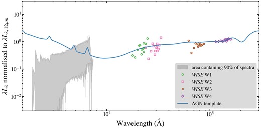
Comparison between SDSS spectra (thin grey lines), WISE derived luminosities (coloured points) and the AGN spectral template (solid blue line) from Assef et al. (2010).
6.3.5 High intrinsic accretion rate AGN
An anticorrelation between [O iii] and the relative intensity of Fe ii has been shown in analyses of emission-line and accretion properties of AGN (Eigenvector 1; e.g. Boroson & Green 1992; Shen & Ho 2014). This relationship can be explained by differences in Eddington ratio – an intrinsically high-accretion rate could be associated with a low [O iii] luminosity. To assess the plausibility of the scenario for statistically significant numbers of the OQQ population, accurate measurements of the black hole (BH) masses would be needed; while this is out of the scope of this paper, analysis of NIR broad lines that may be less obscured (e.g. NIR measurements; Onori et al. 2017b) could provide the necessary information. Results from OQQ J0751+4028 do not support this (Greenwell et al. 2021, 2022), as it is not luminous enough to imply a sufficiently high Eddington ratio.
6.3.6 Other IR-selected quasars
Using the WISE– WISE colour plane, as done here for OQQs, Hviding et al. (2018) focus on a different region of the plane, choosing targets more likely to be heavily obscured. They also make no selection based on emission lines, and the majority of their sources appear more optically typical than the OQQs. However, while there is no direct overlap between these samples, they are likely to be close cousins with unusually heavy obscuration instead of unusually distributed. Further investigation of the targets with insufficient spectral lines or features to assign a spectroscopic redshift leads Hviding et al. (2018) to hypothesise that a subset of these may be powerful AGN with emission lines attenuated by thick line of sight obscuration.
Extremely Red Quasars (ERQs) are quasars that show an unusually high IR to optical ratio (e.g. Banerji et al. 2015; Glikman et al. 2022). Ross et al. (2015) select these objects based on a comparison between SDSS and WISE magnitudes, producing a sample of objects up to z ∼ 4. An interesting subset of these, at z ∼2–3, show extremely broad emission lines which are not easily explained by current models. Some of these ERQs could be a Type 1 analogue to ‘cocooned’ OQQs – i.e. sources with a high covering factor (not the complete 4π steradians) and possibly obscuring material on large scales, but that retain some (unobscured but possibly reddened) line-of-sight to their nucleus; therefore presenting with broad AGN emission lines. Spectropolarimetry results from Type 2 ERQs (Alexandroff et al. 2018) indicate that the visible emission lines are due to reflection from a dusty disc wind rather than a direct line-of-sight. A potential interpretation is that these are similar to ‘cocooned’ OQQs, but with a small opening that allows the opportunity for reflected emission to be visible. Furthermore, an attempt at OQQ selection in large surveys based on photometry alone or low-quality spectroscopic data may include a number of ERQs, therefore it is important to understand their physical differences and how they might be distinguished.
Another interesting population found with extremely high infrared luminosities are Dust Obscured Galaxies (DOGs). These objects are selected based on an excess of 24 μm (from Spitzer; Dey et al. 2008) or 22 μm (from WISE; Toba et al. 2015) emission compared to optical, and are thus selected to be underluminous in the rest-frame UV. They often show signs of intense star formation or obscured AGN activity (Dey et al. 2008; Toba et al. 2017), with MIR colours indicating AGN presence in a large number of them, particularly at higher luminosities (Toba & Nagao 2016; Toba et al. 2017). The high luminosity along with dust obscuration seem to place them into the high-growth post-merger phase of the galaxy merger scenario for AGN-host galaxy growth (Hopkins et al. 2008). Their selection process results in a subset of DOGs that lack broad emission lines, and thus may be closer to OQQs than Type 1 ERQs. However, evidence of star formation and the presence of strong narrow lines shows that they are not an identical population. Spectropolarimetry results may suggest an evolutionary connection between ERQs, Hot DOGs, and other reddened quasars (Assef et al. 2022).
Glikman et al. (2012) select candidate red quasars based on 2MASS (IR) and FIRST (radio) data. A detailed examination of the radio properties of OQQs is outside the scope of this paper, but we searched the FIRST catalogue (Becker, White & Helfand 1995) and found 7 FIRST counterparts to OQQ candidates, of which four are brighter than 10 mJy at 1.4 GHz. The OQQs are therefore not consistently radio bright or dim, and unlikely to be similar, population-wise, to radio-selected objects.
6.3.7 Blazars
One potential source of contamination in this sample is likely to be blazars – the chance viewing of AGN head on to a relativistic jet (Landt et al. 2004), producing a bright, variable source, strong in radio emission. These are known to be very bright objects, with some exhibiting very flat spectra. As such, there may be a number that pass the criteria specified in Section 3, but that are not relevant objects for this paper. It would be useful therefore to be able to estimate the level of such contaminants in our sample, and if possible to remove some in order to improve the reliability of the sample.
D’Abrusco et al. (2014) created a catalogue of γ-ray emitting blazars, assembled from WISE sources. Comparison of overlapping sources from this catalogue (WIBRaLS) with our OQQ sample, and with respect to various parameters, could help identify the unwanted objects. Massaro et al. (2012) identified the WISE Gamma-ray Strip (WGS), which uses IR colour–colour diagrams to distinguish possible blazars. They divide these into two sub-categories – BZBs (BL Lac objects, with featureless optical spectra – galactic absorption lines or weak emission lines only), and BZQs (flat spectrum radio quasars, where the optical spectrum should show broad emission lines). According to these definitions, the most likely category for any contaminant objects will be BZB. Massaro et al. (2012) quantify the likelihood of a source being within the WGS, based on its location on three WISE colour–colour diagrams, and the uncertainties on those colours. Fig. 16 shows the application of this method to our objects. This is not considered a sufficiently reliable classification to remove any sources from the OQQ list, merely to assess the level of contamination from BZB sources.

Furthermore, given the flat spectrum characteristic of blazars, they tend to have weak values of D4000. Fig. 8 shows that the OOQs tend to show significant breaks, and this can be seen in the individual optical spectra (Fig. A). Hence, a visual check of the spectra substantially reduces the likelihood of blazar contamination (Section B2).
One property common to all blazar types is that they exhibit high, irregular variability across the whole spectrum. As such, this may be a useful way to distinguish likely blazars from OQQs.
After the completion of the main WISE mission, the NEOWISE project (Mainzer et al. 2011) continues to scan the sky, doing so approximately every six months (depending on sky location) with the W1 and W2 bands (W3 and W4 cannot operate without cryogenic cooling, and this was exhausted during the main phase). The primary science aim of this phase is the study of near Earth objects. However as the single exposure images and source magnitudes are available from the NEOWISE database15, it provides a measure of the multi-year timescale infra-red variability.
To approximately quantify the level of variability in each source, the data from each WISE measurement epoch was averaged, then these combined points fit to a time-invariant line. χ2 was used to assess whether this invariant state could reasonably explain the observed variation in WISE detections16 If it could not, then intrinsic uncertainty was added to the points. The size of this intrinsic uncertainty was used as an estimate of the variability of the source, and Fig. 17 shows the results of this. Fig. 18 shows the fitting with the OQQ showing highest variability, OQQ J1208+1159. This source is flagged as a WGS BZB (see Fig. 16), and is detected in FIRST (Becker, White & Helfand 1995) as a compact source with integrated flux 67.31 mJy. This combined with the MIR variability suggests that it may be a blazar.
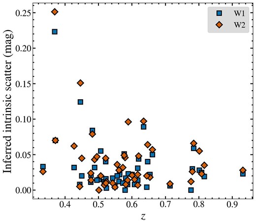
Intrinsic spread added to force the WISE data to be consistent with an unvarying source – higher values indicate that the source is more variable, and less likely to be stable.
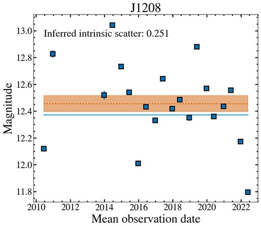
W2 variability of the OQQ showing significant variation (>0.1 mag). It appears to show random variability, although the large time-steps in available WISE data make statistical assessment of the variability difficult.
The number of objects found that are above the threshold for being within the WGS BZB is 17 out of 47 OQQ. The number of objects with matches in the WIBRaLS table is 8 out of 47 OQQs—these are all also above the BZB threshold. The number of objects with high variability is currently difficult to quantify without a comparison threshold. The QSO2 variability is slightly lower on average (mean 0.031/median 0.020 for OQQ, mean 0.026, median 0.017, for QSO2s) and includes no very high variability objects.
If we take the lower limit of high variability as 0.1, then there are two OQQs above this threshold, both of which are likely BZBs. Of the 47 OQQs below the threshold, 36 per cent are likely BZBs. In comparison, 57 QSO2s (out of 1,990; 2.9 per cent) pass the BZB threshold overall. An examination of the variability of a large sample of non-AGN and various types of AGN would be illuminating, but outside the scope of this work. Due to the high uncertainties on these methods, it is difficult to fully quantify the number of BL Lac objects that could be interfering in the results here: anything from 3 per cent to 25 per cent may be possible.
6.4 Evolutionary context
It is important to consider the cosmological situations where we might find OQQs. Many works have examined the life cycle of galaxies and AGN during mergers (e.g. Di Matteo, Springel & Hernquist 2005; Springel, Di Matteo & Hernquist 2005; Hopkins et al. 2006). As the two galaxies interact, the interstellar medium from both comes together, and the resultant enhanced density of matter leads to increased star formation, and (as the bulk of the merging galaxy reaches the nucleus of its pair) we may see increased AGN activity. This brightening starts as the AGN is still enshrouded in dust and gas from the merger, but as the emission increases in intensity, energy and matter feedback starts to clear out the obscuring matter. Our OQQ sample objects, for the most part, do not show signs of high SFR as may be expected if they lie in this part of the sequence. Thus, OQQs do not obviously fit the standard paradigm for AGN and host galaxy evolution.
Springel, Di Matteo & Hernquist (2005) show that in a modelled merger of two disc galaxies, including AGN feedback and BH growth, the peak of SFR precedes the black hole accretion rate (BHAR) peak by a small amount of time. SFR begins to drop before the BHAR, so there may be a short period of time where the SFR is well below peak, but BHAR is high. As BHAR is proportional to AGN luminosity, the OQQ objects might be objects in this short transitional phase. We find fewer OQQs compared to QSO2s, suggesting that the OQQ duty cycle is shorter than the duty cycle of Type 2 quasars. Interestingly, the difference in median redshift between these two samples (e.g. Fig. 2) implies that there may be genuine evolutionary differences between their populations, with OQQs peaking earlier than QSO2s. However, incompleteness issues could impact both source samples at the upper redshift end, and the number of nearby OQQs may be artificially low simply due to easier detectability of faint [O iii].
The two galaxies are coalescing at this point so would not necessarily be clearly identifiable as advanced mergers, especially with the images currently available. Additional high resolution imagery could be valuable in identifying any late stage mergers among the sample. For the OQQs to be objects existing in this brief period of time, we may expect strong outflows to be visible, if the SFR is being quenched by AGN activity. These will manifest as blueshifted absorption lines, or broadened and asymmetric emission lines at the systemic velocity of the source. With the current spectra this is impossible to either confirm or rule out, but measurements of select likely candidates with more sensitive instruments could provide more insight into these scenarios.
Simulations by Blecha et al. (2018) suggest that MIR selection of AGN in mergers may miss AGN, particularly low apparent luminosity and very late stage mergers. This work selects for high IR luminosity objects in order to produce a more reliable candidate list; lower luminosity OQQs may be missed from MIR selection due to (a) selection being less complete in general for less bright objects, (b) as shown in Blecha et al. if OQQs are late stage mergers.
The absence of obvious merger signatures may instead point towards high-mass ratio mergers, with the smaller galaxy not massive enough to significantly disrupt the morphology of the larger primary, nor massive enough to trigger substantial star formation throughout the body of the primary. However, an efficient mechanism to channel the gas from the donor galaxy to the central SMBH would be required in this case. Alternatively, whether secular processes such as efficient gas flows can trigger AGN activity without simultaneous star formation remains unclear.
Alternatively, the ‘Young AGN’ scenario presents a different evolutionary perspective. If the triggering event is recent enough, the AGN could be switching on, mimicking the phase described by Schawinski et al. (2015) as ‘Optically Elusive AGN’. They show that there could be a period of ∼104 yr in which the AGN is visible in X-rays but has not yet photoionized the extended area that will later become the NLR. As the dusty torus (the source of reprocessed IR emission, and the IR colour that we select for in this work) is closer to the central engine than the NLR, we expect that sign of AGN life to appear prior to any narrow optical emission lines.
Schawinski et al. (2015) calculated the full duty cycle of an AGN as ∼105 yr, and the optically elusive phase as ∼104 yr. If we expect the IR bright OQQ phase to be some fraction of the optically elusive phase, this puts the OQQ lifetime at less than ∼10 per cent of the ‘normal AGN’ duty cycle. The viewing angle of OQQs and QSO2s is likely to be similar – both viewed through the torus, obscuring any broad emission lines – so assuming they have similar covering factors, we would expect to see them in the same proportions as the full range of AGN types: approximately 10:1. We find ∼1000 QSO2s and 47 OQQs: approximately 20:1; encouragingly close, but somewhat fewer OQQs than expected, especially if we consider that some OQQs may be ‘cocooned’ rather than ‘young’. As stated above, however, the 10:1 ratio is a lower limit, based on the full ‘optically elusive’ timescale. If every OQQ is a ‘young AGN’ our results are consistent with the IR bright stage being approximately two thirds of the ‘optically elusive’ phase. These are merely crude estimates that do not fully account for selection and modelling biases, much of which remain unknown.
An investigation of the morphologies of OQQs could provide some interesting insight into their relationship with their host galaxies; for example, Rigby et al. (2006) found from an examination of the morphologies of X-ray–selected optically dull AGN that such sources exhibited a wider range of axis ratios (major–minor axis, assuming an elliptical shape) as compared to optically active AGN which showed only very round axis ratios. They conclude that extranuclear dust within the host galaxy is responsible for an optically dull nature. SDSS photometry is severely limited for this purpose and is unlikely to be able to accurately resolve the size or axis ratio of the host galaxy except in unusual cases. Future surveys, such as Euclid (Euclid Collaboration et al. 2022), will greatly improve on this.
7 SUMMARY
By selecting MIR–luminous sources with red WISE colours and a marked absence of optical emission lines, we have presented a new sample of quasars that are candidates for being enshrouded within dust cocoons. The overall sample shows broad-band continuum properties very similar to those of SDSS-selected QSO2s, but with an [O iii]λ5007 emission line suppression factor of |$\gtrsim$|250 (see Section 4.3). We show that host galaxy dilution is unlikely to be a major effect in most cases.
The idea of fully enshrouded AGN is far from new. Various models suggest that the bulk of AGN growth occurs in highly obscured phases (e.g. Fabian & Iwasawa 1999; Hopkins et al. 2006). The shape of the cosmic X-ray background spectrum also requires similar numbers of Compton-thick (NH> 1024 cm−2) obscured AGN compared to unobscured. Ananna et al. (2019) calculate the required proportion at z = 1.0 as 56 per cent ± 7 per cent (50 per cent ± 9 per cent at z = 0.1). A number of dedicated legacy surveys with NuSTAR that are selected in the infrared are finding CT fractions ≳30 per cent within ≲200 Mpc (e.g. the NuSTAR Local AGN NH Distribution Survey – NuLANDS, Boorman et al. in preparation), and the [Ne V] survey; Annuar et al. 2020). In any evolutionary paradigm, this would naturally include fully obscured sources in the stochastic competition between gas feeding from large scales and AGN feedback, especially if there is a delay between the two competing processes (noting that NuLANDS currently includes optical classification as part of the sample definition; the preliminary infrared selection should still include such fully covered objects). It may also imply the existence of obscured objects that do not occur as part of the merger-driven growth phase, but instead represent a separate path.
The receding torus model also suggests that the covering factor of AGN decreases with luminosity (e.g. Lawrence 1991) so fully covered AGN may be more likely to occur at low AGN luminosities. This issue is far from settled, however, with conflicting results from a variety of studies in different bands (e.g. Glikman et al. 2007; Lawrence & Elvis 2010; Toba et al. 2014; Assef et al. 2015). An element of bias can be introduced by requiring that optical emission lines be present for secure source redshift and type identification – any sample based on this selection criteria may be missing objects with some emission lines blocked, either completely or to a level below measurable. The strength of our selection criteria is to instead rely upon the reprocessed thermal spectrum (i.e. MIR colours) and luminosities, allowing us to search for objects in which potential 4π or near 4π covering completely extinguishes the optical lines.
We show that unknown AGN with unusual properties can be selected with a combination of multiwavelength selection techniques, finding 47 ‘Optically Quiescent Quasars’ (OQQs; strong MIR objects with no [O iii] emission) – see Section 3.
Comparisons with Type 2 quasars (QSO2s; similarly MIR bright, but selected for strong narrow [O iii]) show similar underlying properties in e.g. redshift, colour, and luminosity distributions, but fewer numbers of OQQs – see Section 3.2.
The exception to this is a strong deficit between the detected [O iii] emission from QSO2s and the upper limits placed on the OQQ lines – see Section 4.3.
We consider what physical explanations may produce the observed properties (Section 6.2), principally:
‘Cocooned’ AGN – an accreting black hole entirely shrouded in obscuring material.
‘Young’ AGN – a recently switched on AGN, resulting in contrasting signals originating at different distances from the black hole.
Intrinsically weak lined AGN – some properties of the accretion disc can cause ionization of narrow lines to be less prominent.
Comparisons with other populations of AGN show that OQQs do not fit into any of these groups, but may be similar to some, depending on their intrinsic nature – e.g. Weak Line Quasars may be similar to OQQs that are caused by unusual accretion activity that results in low ionization; Compact Obscured Nuclei may be similar to ‘cocooned’ AGN – see Section 6.3.
ACKNOWLEDGEMENTS
We would like to thank the referee for their helpful and constructive feedback. This research is funded by UKRI. CG received support from a University of Southampton Mayflower studentship and Durham University CEA STFC grants, numbers ST/T000244/1 and ST/X001075/1. PG acknowledges support from STFC and a UGC-UKIERI Thematic partnership (STFC grant number ST/V001000/1). PGB acknowledges financial support from the Czech Science Foundation project No. 22–22643S. WISE is a project of Univ. California, Los Angeles, and Jet Propulsion Laboratory (JPL)/California Institute of Technology (Caltech), funded by the National Aeronautics and Space Administration (NASA). Funding for SDSS-III has been provided by the Alfred P. Sloan Foundation, the Participating Institutions, the National Science Foundation, and the U.S. Department of Energy Office of Science. The SDSS-III web site is http://www.sdss3.org/. 2MASS is a project of the Univ. Massachusetts and the Infrared Processing and Analysis Center/Caltech, funded by NASA and the National Science Foundation. This research has made use of data obtained from the Chandra Data Archive and the Chandra Source Catalog, and software provided by the Chandra X-ray Center (CXC) in the application packages CIAO and Sherpa. This work made use of observations obtained with XMM–Newton, an ESA science mission with instruments and contributions directly funded by ESA Member States and NASA. This research made use of data from the NuSTAR mission, a project led by the California Institute of Technology, managed by the Jet Propulsion Laboratory, and funded by NASA. This research has made use of the NuSTAR Data Analysis Software (NuSTARDAS) jointly developed by the ASI Science Data Center(ASDC, Italy)and the California Institute of Technology(USA). The NASA/IPAC Infrared Science Archive (IRSA) operated by JPL under contract with NASA, and SIMBAD operated at CDS, Strasbourg, France, were the main databases queried. The USNO Image and Catalogue Archive is operated by the U.S. Naval Observatory. This research has made use of data obtained through the High Energy Astrophysics Science Archive Research Center Online Service, provided by the NASA/Goddard Space Flight Center. This research made use of astropy17, a community-developed core Python package for Astronomy (Astropy Collaboration et al. 2013, 2018). Many thanks also to Taiki Kawamura for his helpful comments and suggestions.
DATA AVAILABILITY
The data underlying this article are publicly available from the WISE All-Sky Survey, SDSS DR15, and X-ray data from the HEASARC archive.
Footnotes
Defined as galaxies that have significant emission at radio wavelengths; radio (5GHz) to optical (B-band) ratio |$\gtrsim$|10 (Kellermann et al. 1989)
3252 of these have W1 magnitude=9999, i.e. are not usable.
With the use of ‘quasar’ in this paper we are referring to high luminosity AGN rather than Type 1 AGN.
1.235 μm, 1.662 μm, 2.159 μm.
Herschel bands used were any available out of 250 μm, 350 μm, and/or 500 μm. Of these nine sources: two have 2MASS only; five have some combination of 2MASS and Herschel; two have Herschel only.
The W3 (12 μm) band magnitudes were chosen as most representative of the region of interest. A more detailed investigation would examine the effects with luminosities rather than magnitudes.
References
APPENDIX A: SOURCE SPECTRA
This section presents the SDSS spectra of a sub-sample of OQQs at rest-frame wavelength in Fig. A1. All spectra are available online.
![SDSS spectra of the first eight OQQs by RA, smoothed to show the continuum shape of each spectrum. Dashed lines in dark red mark key features: the 4000 Å break (see Section 4.5), [O iii], and H $\alpha$. Full sample available online.](https://oup.silverchair-cdn.com/oup/backfile/Content_public/Journal/mnras/527/4/10.1093_mnras_stad3964/1/m_stad3964figa1.jpeg?Expires=1749806887&Signature=4YcW4XewpYFdSQSLJLrV-zQ0b04~ST6bylJ2qgoNGzxz3u1eU4lh4BtoQY6LitxCHLLFyfcJNruTYLvPPuBa0uSma7USoYtN~DaeSD4lvXQuiLWu1Z7Aezpxx4ftsScv2z0ekV-3n8ez1-qKAzJFLuIuXxL-SQcVPV4BEyNBEdv-yXsTwgZZknSmGB5QxyoN884ROLctItKhgLp0kQkKFTPWdHFFZh46qHQMwfg-8DhtNfpC44QbR4iaf5JYEGqVKMU23cLqzLL-e9tkOeVu9T9gEQ3T0YTGQan8qnHUt9OxVefzGOFjvG~fL6b7yPUOhoD5egzmf1w0hSgBNCfWMA__&Key-Pair-Id=APKAIE5G5CRDK6RD3PGA)
SDSS spectra of the first eight OQQs by RA, smoothed to show the continuum shape of each spectrum. Dashed lines in dark red mark key features: the 4000 Å break (see Section 4.5), [O iii], and H |$\alpha$|. Full sample available online.
APPENDIX B: SPECTRA SELECTION
B1 [O iii] Line Presence Elimination
We start with the primary SDSS spectrum for each OQQ candidate, which was cut down to the region around the [O iii] doublet (rest-frame wavelength 4860 to 5100 Å – see Fig. B1). We aim to find upper and lower bounds for a fit to the [O iii] line, based on a Gaussian on top of a straight line. In Reyes et al. (2008), they used a double Gaussian fit to find the presence of strong [O iii]. However, we found that due to the low level of our target [O iii] lines, the second peak caused the fit to be confused by the noise. We therefore fit only one Gaussian. Next, we assess the uncertainty on the line flux, with the aim of checking whether the lower bound is less than zero, and hence whether only an upper bound can be placed on the emission. The continuum can be ignored in this simulation, as it cancels out from the equation. Finally, we select OQQs from the candidate objects that pass all other tests (as outlined in Section 3).
![Full spectrum, showing cut out with the region used in the fits. Purple + markers show the possible location of any spectral lines. Red star marker shows the location of [O iii]. Vertical shaded regions show emission lines cut for the fit. Bottom right panel shows the region used for SNR calculations. Vertical shaded areas show the SNR estimate regions. Noise is estimated from these and compared to the continuum flux, as described in Section B3.](https://oup.silverchair-cdn.com/oup/backfile/Content_public/Journal/mnras/527/4/10.1093_mnras_stad3964/1/m_stad3964figb1.jpeg?Expires=1749806887&Signature=hUfwIClhJ3UYfYTW1Mz2~qUzDwFvEAfGtoowG-EdQHpLkwj7DrAgDBGJCESaa0YqmvTH3Jtvzx~i~93oQXfqQVUyzjBBih5DzhjUnVXIfuDtTUflTiloz9uTdHZyMdS7jSyLX5zGhkDtG5KszgvviCm94kgtKoZfZBWxKaOxnoevVqmCsbwCj2Waagab~8ssfPU7g-npZBjw~2JhvTvJwOmxlsPsfgjjpFO7YgsQTDg7ukkkEWB7W9SZEivRnhSg110CnvOXSabNjU9SdBf9~qpbu4mtlpPwcvOY0NnCEiKksmaY-MdGtuGb8cYGZexxCtIWzdaxPJXfEDo4bGu-VQ__&Key-Pair-Id=APKAIE5G5CRDK6RD3PGA)
Full spectrum, showing cut out with the region used in the fits. Purple + markers show the possible location of any spectral lines. Red star marker shows the location of [O iii]. Vertical shaded regions show emission lines cut for the fit. Bottom right panel shows the region used for SNR calculations. Vertical shaded areas show the SNR estimate regions. Noise is estimated from these and compared to the continuum flux, as described in Section B3.
Method:
cut to local region around [O iii] line wavelength (see Fig. B1)
Set bounds for all parameters (see Table B1)
Remove regions where any spectral lines other than [O iii] would be found, if present (see Fig. B1)
Fit function to data (y = mx + c + gaussian(x0, σ, h))
Simulate an [O iii] line for parameters randomly selected from their uncertainty bounds
Calculate line flux for each simulated line
Look at lower bound on line flux from simulations – if less than zero, we can conclude that the line only has an upper limit (Fig. B2 shows spectra for a selection of [O iii] detected and non-detected candidates)
Select subset to pass onto the next step.
![Candidate OQQs, randomly selected from the catalogue at Step 8 (see Table 2). Labelled in green (‘[O iii] not detected’) show the objects that pass this test and move on to visual checks, and those labelled in red (‘[O iii] detected’) are discarded. Grey sections of the spectra show regions removed for this test to avoid other possible emission lines biasing the fit.](https://oup.silverchair-cdn.com/oup/backfile/Content_public/Journal/mnras/527/4/10.1093_mnras_stad3964/1/m_stad3964figb2.jpeg?Expires=1749806887&Signature=XwKTsjEb00gpIrlj4owqexKVHLXvz8XRxdvu0EGifujSgnvP1XDQTA0vMe0kHrBIiRi2CkvWSzbXLJOwC4QLG8I9cw4CM06hKerloaoh4o03INb8JzfAsCPaHQr-UoLoVsiGdvNXxo7kUnMkujrhgFzgCA3T41CspOhia9x9c2pkDhG8PQRpnCqZazFA6~nFfvjZ-Ou-OfWQvV2jwpa4cVTEtLld7sWaCk1DtgM0aAPyBpNWS-wz4BJ-oprNdpROYHxjjVu5zAJoRktGxDOOxtb-cPmh7zomvwod0aMBpo~tnD3dwBIAm9QBujsBLMt9Xll-futVcP0-5bKG6xHzxw__&Key-Pair-Id=APKAIE5G5CRDK6RD3PGA)
Candidate OQQs, randomly selected from the catalogue at Step 8 (see Table 2). Labelled in green (‘[O iii] not detected’) show the objects that pass this test and move on to visual checks, and those labelled in red (‘[O iii] detected’) are discarded. Grey sections of the spectra show regions removed for this test to avoid other possible emission lines biasing the fit.
Bounds imposed on fit parameters. Slope and intercept of background continua were allowed to vary freely, whereas parameters of the Gaussian fit to the emission line were restricted to physically likely values.
| Parameter | Symbol | Bounds |
|---|---|---|
| Slope | m | none |
| Intercept | c | none |
| Line wavelength/Å | x0 | up to 1000 km s−1 from centre |
| Line FWHM/Å | σ | physical min up to 500 km s−1 |
| Line height/flux units | h | max based on data |
| Parameter | Symbol | Bounds |
|---|---|---|
| Slope | m | none |
| Intercept | c | none |
| Line wavelength/Å | x0 | up to 1000 km s−1 from centre |
| Line FWHM/Å | σ | physical min up to 500 km s−1 |
| Line height/flux units | h | max based on data |
B2 Visual check
All spectra that passed the automatic check were then inspected by eye, and discarded or flagged based on several criteria. These cuts were done with the aim of making a highly reliable rather than complete sample, so that we are as certain as possible about the relevant nature of each passing candidate. A summary of these results is shown in Table B2.
Counts of objects removed or kept at all stages of checks outlined in this Appendix.
| Original candidates | % | |
|---|---|---|
| Total | 1,520 | |
| Lower bound flux < 0 | 203 | 13.4 |
| Keep (after basic vis check) | 98 | 48.3 |
| Remove (visible [O iii]) | 48 | 23.6 |
| Remove (noisy) | 42 | 20.7 |
| Remove (wrong class) | 14 | 6.9 |
| Keep (after detailed vis check) | 64 | 64.3 |
| Uncertain redshift | 20 | 20.4 |
| Poor S/N | 12 | 12.2 |
| Wrong shape continuum | 3 | 3.1 |
Visible [O iii] – the automatic check sometimes fails to find a significant [O iii] signal, despite there being a small but clearly apparent peak. We visually examine each spectrum, and based on the region around [O iii] and the width and height of the visible peak, we discard or keep objects based on whether the [O iii] seems truly absent.
Noisy data – we discard any candidates where the noise in the region of the [O iii] line is visibly worse than the flux there, in order to remove any where the [O iii] is likely to be lost in the noise. The S/N is calculated in detail in a later step (Section B3)
Incorrect class – candidates were selected based on SDSS spectroscopic classifications, but rarely an object is misclassified, and we discard any objects where the class appears unreasonable.
Uncertain redshift – candidates were already selected based on SDSS spectroscopic redshift showing no warning, but this automatic fit fails occasionally. We discard any objects where it is not clear how the redshift has been assigned.
By design, the OQQ spectra show no [O iii], and as shown in Fig. 6, H |$\alpha$| is also generally low, where measurable. However, some optical spectra show other indicators of AGN presence and/or other interesting features.
Blue continuum shapes: although any sources with extremely blue spectra were removed in Section 3, some remain with a blue upturn below the |$4000 \,{{\mathring{\rm A}}}$| break (for example, sources shown in Fig. B3, top), which may indicate some contribution to the continuum from the accretion disc. This is a small number of sources and are unlikely to represent a major part of the OQQ population, but the combination of continuum shape and lack of emission lines may make these interesting sources. Alternatively, this blue emission could be due to recent star formation, especially if seen in combination with other signatures such as [O ii].
Broad emission lines: generally emission lines are low level or narrow for the majority of the sample, but there are some exceptions. J0948+0958 in Fig. B3 (middle) shows broad H |$\alpha$| emission, possibly implying a source with greater velocity dispersion than expected from the galaxy, and likely AGN-related. Hα is present in several more sources but generally less broad. It is outside of the clean spectroscopic range for a large proportion of the OQQs, making judgement of population properties in this case harder.
SF versus dead galaxy indications: some SED fitting shows a contribution to MIR luminosities from SF (see Section 4.4), but only a small fraction of OQQs have sufficient data to draw reliable conclusions about their properties from these fits. Nevertheless, it implies that not all of the OQQs are dead galaxies with very little star formation, and observed properties of some spectra also lead to this conclusion. Narrow emission lines such as [O ii] may indicate a younger stellar population and thus recent or ongoing star formation, and some sources (e.g. sources in Fig. B3, bottom) may show this. A strong 4000 Å break and Ca H and K absorption lines could instead imply an older population. However, as discussed in Section 4.5, this may not be conclusive.
![OQQ spectra showing selected spectra with the following properties: (top) spectra showing blue rises, (middle) spectra showing strong and/or broad Hα emission, (bottom) spectra showing narrow [O ii] emission.](https://oup.silverchair-cdn.com/oup/backfile/Content_public/Journal/mnras/527/4/10.1093_mnras_stad3964/1/m_stad3964figb3.jpeg?Expires=1749806887&Signature=siOH6UpP2lXehifdBGpPDjwxBhDuKR-ueOWecNbwYXOVffCL2zNMMSmdGMXSCxNDY1i3dwLSZDgG~pvwQbVK~xuANG5-JQFNC8wY3mv68EMo9jk-xPIu4yu2X4J1N3dfFn7NU3ba17vF9v-Om2vq~QSnsHMuQXpvXySXcUUue4-PY7K~Y40m44m-alZXzIx~2MpFek21ywC7988-j3y~OXpOnXxFPb~y~8xhMyglLvMvcBdSmDAGoysPQt7PkNSI3UkK1iG50NgX4Qo8kDOFKMnkEnoQTEDyV5DRPr0xPA7d~LkxhyqB5ebpjCXavRR8JBlx9AleroR0qc8cYZeeVg__&Key-Pair-Id=APKAIE5G5CRDK6RD3PGA)
OQQ spectra showing selected spectra with the following properties: (top) spectra showing blue rises, (middle) spectra showing strong and/or broad Hα emission, (bottom) spectra showing narrow [O ii] emission.
We can conclude from inspection of the spectra (along with other properties) that it is unlikely that OQQs represent a single intrinsic type. Rather, it is more likely that they represent multiple classes that, due to obscuration or accretion properties, appear similar in terms of OQQ selection (see Section 6.2). Future work is needed to effectively and conclusively distinguish between intrinsic properties.
B3 Continuum SNR check
To eliminate sources where the spectrum in the region of [O iii] is significantly noisy – i.e. that there may be [O iii] present at a low level – we estimate the noise as follows (summary of results in Table B2 as ‘Poor S/N’):
Cut the spectrum to two regions on either side of the expected position of [O iii] (vertical bands in Fig. B1, bottom right panel), avoiding any other potential emission or absorption lines.
Estimate the noise in these regions as the standard deviation on the flux data.
Estimate the signal as the mean on the flux data.
Discard any candidate OQQ with the ratio of these >2.
B4 Duplicate spectra
For the fitting and selection process, and the properties in the main sections of the paper, we use only the spectra assigned by SDSS as SciencePrimary (a flag that indicates that this spectrum is considered the best available for this source). However, for a minority of sources there are multiple spectra available, so we compare these to see if there is any significant difference in flux, class, redshift, or emission line flux.
Most of these duplicate spectra are either well matched, or are candidates that are dismissed for high levels of noise. We discuss the exceptions to this below.
B4.1 J0002: 0.592036, -0.4320923
Two available spectra; generally consistent in appearance and flux, but one has been assigned the SDSS subclass ‘Star-forming’ (our selection process requires subclass ‘null’). This may be due to a change in emission line height. We choose to keep this candidate based on its otherwise promising appearance.
B4.2 J0231: 37.99002, 0.648491
Fifteen available spectra; generally consistent in appearance and flux, but again one has been assigned the SDSS subclass ‘Star-forming’. We also choose to keep this candidate based on its otherwise promising appearance; as the potentially star-forming galaxy is only one of the available spectra, and the rest are ‘null’, as required.
B4.3 J0911: 137.96392, 29.824825
Three available spectra. All with consistent SDSS class and redshift, but clear changes in flux between spectra, particularly noting a change in shape in one. The primary spectra is the most recent, so we have retained this object in the sample, but note that it may be variable.
APPENDIX C: COLOUR IMAGES
This section presents PanSTARRS colour images of a sub-sample of OQQs in Fig. C1. The full sample is available online.
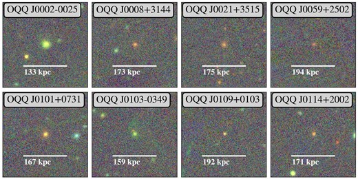
PanSTARRS colour images of the first 8 OQQs by RA. Bars show approximate scale of objects based on redshift. Full sample available online.
APPENDIX D: X-RAY DATA SOURCES
Here we summarize the source papers used for QSO2 X-ray information and observation IDs of OQQ data used in Section 5.
| Name (1) | RA (J2000) deg. (2) | Dec. (J2000) deg. (3) | log L12erg s−1 (4) | log L2 − 10 keV erg s−1 (5) | log |$L_{\rm {[O\, {\small III}]}}$| L⊙ erg s−1 (6) | log NHcm−2 (7) | Reference (8) |
|---|---|---|---|---|---|---|---|
| WISEA J012341.47+004435.8 | 20.923 | 0.743 | 44.83 | 44.53 | 9.13 | 23.16 | (b) |
| WISEA J080154.26+441234.0 | 120.476 | 44.209 | 45.04 | 44.62 | 9.58 | 23.63 | (a) |
| WISEA J081253.10+401859.9 | 123.221 | 40.317 | 45.05 | 44.23 | 9.39 | 22.33 | (b) |
| WISEA J083945.98+384318.9 | 129.942 | 38.722 | 44.97 | 44.26 | 9.71 | 22.52 | (c) |
| WISEA J115314.38+032658.6 | 178.310 | 3.450 | 45.04 | 44.08 | 9.61 | 22.19 | (a) |
| WISEA J122656.47+013124.3 | 186.735 | 1.523 | 45.30 | 44.63 | 9.66 | 22.42 | (a) |
| WISEA J122845.73+005018.8 | 187.191 | 0.839 | 45.11 | 43.54 | 9.28 | 23.18 | (b) |
| WISEA J164131.72+385840.7 | 250.382 | 38.978 | 45.48 | 44.87 | 9.92 | 22.74 | (a) |
| Name (1) | Instrument (2) | Observation ID(s) (3) |
|---|---|---|
| OQQ J0002-0025 | Swift-XRT | 38112001,38112003,38112009,38112002,38112007,38112008,38112005,38112006,38112004 |
| OQQ J0109+0103 | Swift-XRT | 47886001 |
| OQQ J0231+0038 | XMM–Newton | 652400801 |
| OQQ J0751+4028 | XMM–Newton, NuSTAR | 0884080101,60701009002 |
| OQQ J1051+3241 | XMM–Newton | 781410101,781410201 |
| OQQ J1611+2247 | Chandra | 15679 |
| OQQ J1617+0854 | Swift-XRT | 46227001,46227006,46227004,46227005,46227003 |
