


ABSTRACT
We report on long-term evolution of gamma-ray flux and spin-down rate of two bright gamma-ray pulsars, PSR J2021+4026 and Vela (PSR J0835−4510). PSR J2021+4026 shows repeated state changes in gamma-ray flux and spin-down rate. We report two new state changes, a first one from a low gamma-ray flux to a high flux that occurred around MJD 58910, and a second one from high to low flux that occurred around MJD 59510. We find that the flux changes associated with these two state changes are smaller than those determined in the previous events, and the waiting time of the new state change from the high gamma-ray flux to low gamma-ray flux is significantly shorter than previous events. Since the waiting time-scale of the quasi-periodic state changes of PSR J2021+4026 is similar to the waiting time-scale of the glitch events of the Vela pulsar, we search for the state change of the gamma-ray emission of the Vela pulsar to investigate the possibility that the glitching process is the trigger of the state change of PSR J2021+4026. For the Vela pulsar, the flux of the radio pulses briefly decreased around the 2016 glitch, suggesting that the glitch may have affected the structure of the magnetosphere. Nevertheless, we could not find any significant change of the gamma-ray emission properties using 15 yr of Fermi-LAT data. Overall, it seems inconclusive that a glitch-like process similar to that occurred to the Vela pulsar triggers the structure change of the global magnetosphere and causes state changes of PSR J2021+4026. Further and deep investigations to clarify the mechanism of the mode change for PSR J2021+4026 are required.
1 INTRODUCTION
Pulsars are highly magnetized and rapidly rotating neutron stars with a stable rotational period. However, there are two types of timing irregularities: glitches and timing noise. A pulsar glitch is defined as a sudden increase in spin frequency. Although the first glitch was discovered over 50 yr ago (Radhakrishnan & Manchester 1969), it remains an area of active research and interest.
In addition to timing irregularity, there are various intriguing phenomena observed in pulsar’s emission, such as mode changes, nulling, intermittency, and pulse-shape variability. It has been inferred that some of the phenomena intimately connect with and arise from alterations in the structure of the pulsar’s magnetosphere. For example, Lyne et al. (2010) report that several mode-changing pulsars, which undergo changes in spin-down states, are accompanied by a clear change in radio pulse profiles. Mode changes in pulsars are evident through alterations in the pulse profile, encompassing changes in the relative intensity, rotational phase, and widths of individual profile components. These transitions are consistently observed in radio pulsars, as documented by studies such as Kramer et al. (2006), Wang, Manchester & Johnston (2007), and Shaw et al. (2022). Mode changes likely signify a clear manifestation of current flow redistribution within the magnetosphere, reflecting alterations in the magnetic field, plasma distribution, or other fundamental elements within this region (Timokhin 2010; Huang, Yu & Tong 2016).
Different time-scales and manifestations of mode changes in radio emission and/or the spin-down rate have been observed. For example, PSR J1326−6700 transits between two radio emission states within a time-scale of the order of ∼100 spin periods (Wang, Manchester & Johnston 2007; Wen et al. 2020), while PSR B2035+36 exhibits one abrupt change in spin-down rate on MJD 52950 over 9 yr observation, and its radio emission after the mode change is transiting between two states (Kou et al. 2018). On the other hand, several mechanisms for mode changes have been observationally and theoretically suggested. For example, connections between the glitching process of neutron stars and mode changes have been observed through radio observations in several pulsars, including PSRs J1119−6127 (Weltevrede, Johnston & Espinoza 2011), and B2021+51 (Liu et al. 2021), in which a new component in radio emission appears or the pulse profile varies following glitches. Keith, Shannon & Johnston (2013) reported a high correlation between variations in the radio pulse profile and the spin-down rate of PSR B0740−28, which is observed subsequent to the glitch occurring on MJD 55022. Kou et al. (2018) reported a possible glitch event coinciding with a mode change of PSR B2035+36.
As most glitching processes of neutron stars do not show the radiative variation, and some mode changes of pulsars occur without any evidence of accompanying glitches, other physical processes have also been suggested to cause mode changes of the pulsars. Precession of neutron stars, which has been suggested as a potential cause for the quasi-periodic changes in the timing residual of PSR B1828−11, exhibits a mode change lasting ∼500 d in one cycle (Link & Epstein 2001; Jones 2012; Kerr et al. 2016; Jones, Ashton & Prix 2017). The impact of an asteroid has been also suggested to explain a significant decrease in spin-down rate and variation of the radio pulse profile that occurred in 2005 September for PSR J0738−4042 (Brook et al. 2014), for which the current spin-down rate still remains lower than the value observed prior to 2005 (Lower et al. 2023; Zhou et al. 2023). Shaw et al. (2022) mentioned that the mode change of PSR B2035+36 is similar to that of PSR J0738−4042. Basu, Melikidze & Mitra (2022) suggested that the evolution of the local magnetic field and the pattern of the sparking discharge in the polar cap acceleration region are causes of the transition between two or more radio emission states.
Variations in emission and mode changes of pulsars have also been observed and investigated with high-energy observations. In particular, since the launch of the Fermi-Large Area Telescope (hereafter Fermi-LAT) in 2008, the known population of gamma-ray pulsars has significantly increased. The all-sky monitoring of the Fermi-LAT enables us to investigate the variability and mode change of the pulsars with the gamma-ray data. PSR J2021+4026 is a radio-quiet pulsar with a spin period of Ps ∼ 265 ms, and it is known as the first variable gamma-ray pulsar. Allafort et al. (2013) reported a sudden decrease in the gamma-ray flux by ∼14 per cent and an increase in the spin-down rate by |$\Delta \dot{f}/\dot{f}\sim 7$| per cent. Subsequent studies (Ng, Takata & Cheng 2016; Zhao et al. 2017) confirmed that the low gamma-ray flux state continues for about 3 yr and returns to the previous high gamma-ray flux state. Takata et al. (2020) found that PSR J2021+4026 switches between two states with a time-scale of several years, namely, a state with high gamma-ray flux and low spin-down rate (i.e. HGF/LSD state) and a state with low gamma-ray flux and high spin-down rate (i.e. LGF/HSD state). Wang et al. (2018) reported that no significant change in the spectrum and the pulse profile in the X-ray band, which are probably originated from the heated polar cap, has been reported (but see Razzano et al. 2023). Besides PSR J2021+4026, Ge et al. (2020) reported the model change in the spin-down rate (∼0.4 per cent) for PSR J1124−5916, which is a radio-loud gamma-ray pulsar, using 12 yr Fermi-LAT data. Although PSR J1124−5916 is a glitch pulsar, the correlated glitch events at the mode changes were not confirmed in the Fermi-LAT data. In X-ray bands, Marshall et al. (2015) found a sudden and persistent increase (∼36 per cent) in the spin-down rate of the radio-quiet pulsar PSR B0540−69, utilizing data from RXTE and Swift telescopes.
With the timing solution obtained from radio observation or Fermi-LAT data, about 50 Fermi-LAT pulsars show glitch activity, and its long-term timing solutions obtained from Fermi-LAT data have been utilized to constrain the glitch mechanisms (e.g. Gügercinoğlu et al. 2022). Lin et al. (2021) investigated the variability of the gamma-ray emission from the glitching pulsar, PSR J1420−6048, and found the spectral variation of the gamma-ray emission between each glitch. Several gamma-ray pulsars with a characteristic spin-down age similar to that of PSR J2021+4026 (τs ∼ 7 × 10⁴ yr) have displayed glitching activities.1 Hence, it is not unexpected that PSR J2021+4026 has also experienced the glitch activities, though such an event has not been confirmed from the long-term timing ephemeris derived from the Fermi-data. Since the mechanism of the mode change for PSR J2021+4026 has not been well understood, further investigation on PSR J2021+4026 and studies on other glitching gamma-ray pulsars will be desired to examine the influence of the glitch activities on the gamma-ray emission properties.
The Vela pulsar (PSR B0833−45/PSR J0835−4510) is associated with the Vela supernova remnant, and was discovered over 50 yr ago in 1968 (Large, Vaughan & Mills 1968). The Vela pulsar is one of the brightest gamma-ray sources in the sky, with a spin period ∼89 ms and spin-down rate ∼1.25 × 10⁻¹³ ss−1. It is known as the first pulsar that was observed to undergo glitch (Radhakrishnan & Manchester 1969) and 24 events have been reported to date (see footnote 1). Among all glitching pulsars, the Vela pulsar shows comparatively frequent glitching activity with a waiting time of ∼3 yr (Dodson, Lewis & McCulloch 2007), and a relatively large glitch size of △ν/ν ∼ 10−6 (Espinoza et al. 2011). Interestingly, Palfreyman et al. (2018) reported a sudden change in the radio pulse shape coincident with the glitch activity on 2016 December 12; an evolution of the pulse profile and polarization was observed in several rotation cycles of the Vela pulsar. The results indicate that the glitch event of the Vela pulsar has an impact on the structure of the magnetosphere. Since the Vela pulsar is one of the brightest gamma-ray pulsars, it is worthwhile to investigate whether the glitch activity causes any variation or state change in the gamma-ray emission.
In this paper, we study the temporal evolution of the gamma-ray emission properties for two bright gamma-ray pulsars, PSR J2021+4026 and Vela pulsar. We created a timing solution for each state of PSR J2021+4026 and for each inter-glitch interval of the Vela pulsar. We compared the pulse profiles and spectra in different time intervals. Section 2 describes the data reduction process for the two pulsars observed by Fermi-LAT. In Section 3, we present the results of our data analysis and report a new state change of PSR J2021+4026. In Section 4, we provide a discussion on the implications of our results.
2 DATA REDUCTION
2.1 Fermi-LAT data
Fermi-LAT is a gamma-ray imaging instrument that scans the whole sky approximately every 3 h, covering the energy band from ∼20 MeV to 300 GeV (Atwood et al. 2009). We selected Pass 8 data in the energy band of 0.1–300 GeV. We choose the position to be RA = 20|$^{\rm h}21^{\rm m}30{{_{.}^{\rm s}}}48$|, Dec. = 40°26′53″.5 for PSR J2021+4026, and RA = 08|$^{\rm h}34^{\rm m}00{{_{.}^{\rm s}}}00$|, Dec. = 45°49′48″.0 for the Vela pulsar. To avoid Earth’s limb contamination, we only included events with zenith angles below 90°. We limited our analysis to events from the point source or Galactic diffuse class (event class = 128) and used data from both the front and back sections of the tracker (evttype = 3). For our spectral analysis, we constructed a background emission model that incorporated both the Galactic diffuse emission (gll_iem_v07) and the isotropic diffuse emission (iso_P8R3_SOURCE_V3_v1) provided by the Fermi Science Support Center. For each bin of spectra and flux evolution, we refit the data by the binned likelihood analysis (gtlike) and estimate the flux.
We have analysed data from the Fermi-LAT instrument taken between 2008 August and 2023 May to study the gamma-ray emission of PSR J2021+4026. Our analysis focused on phase-averaged spectra, in which we divided the entire data set spanning from 2008 to 2023 into six inter-glitch intervals: MJD 54710–55850 (high gamma-ray flux/low spin-down rate state: HGF/LSD 1), MJD 55850–56990 (low gamma-ray flux/high spin-down rate state: LGF/HSD 1), MJD 56990–58130 (HGF/LSD 2), MJD 58130–58970 (LGF/HSD 2), MJD 58970–59510 (HGF/LSD 3), and >MJD 59 510 (LGF/HSD 3). To model the spectrum of PSR J2021+4026, we used a power law with an exponential cut-off, which can be expressed as
The spectral parameters of PSR J2021+4026 include the photon index (γ1), a which is related to the cut-off energy, and γ2, the exponent index.
To study the evolution of the gamma-ray flux above 0.1 GeV, we divided the data into 60-d time bins. The contribution of each background source is calculated with the spectral parameters obtained from the entire data in each bin. Then, we refit the data by the binned likelihood analysis (gtlike) and estimate the flux.
We also performed the likelihood analysis of the Vela pulsar in the time range of 2008 August to 2022 December. We use the power law with an exponential cut-off model as mentioned above, and the data are divided into seven time segments separated by glitches: MJD 54686–55408, MJD 55409–56556, MJD 56557–56922, MJD 56923–57734, MJD 57735–58515, MJD 58516–59417, and MJD 59418–59900. By creating timing ephemeris for each inter-glitch interval, we study the evolution of the gamma-ray flux and examine the pulse profile in different energy bands. This will allow us to determine whether there are any significant changes in the pulsar’s high-energy emission that is associated with glitch events.
2.2 Timing analysis
To ensure that we include the majority of significant source photons, we consider the photon events within a 1° aperture centred at the targets. We assign phases to these photons using the Fermi plug-in for TEMPO2 (Edwards, Hobbs & Manchester 2006; Hobbs, Edwards & Manchester 2006). We barycentred the photon arrival times to TDB (Barycentric Dynamical Time) using the JPL DE405 Earth ephemeris (Standish et al. 1998). This was done using the ‘gtbary’ task, which provides accurate measurements of the positions and velocities of Solar system. To obtain the timing ephemeris, we use the Gaussian kernel density estimation method (de Jager, Raubenheimer & Swanepoel 1986) provided in Ray et al. (2011) to build an initial template. We then use this template to cross-correlate with the unbinned geocentred data to determine the pulse time of arrival (TOA) for each pulse. Once the pulse TOAs are obtained, we can fit them to an original timing model assumed from the semiblind search, the timing results of PSR J2021+4026 and Vela pulsar are shown in Appendix A.
To obtain the temporal evolution of the spin-down rate, we divide the data into several 10-d time bin and determine the first derivative of the frequency for each time bin. We also create the long-term ephemeris for the two states of PSR J2021+4026 and for each inter-glitch interval between two glitch events for the Vela pulsar.
3 RESULTS
3.1 PSR J2021+4026
3.1.1 Temporal evolution
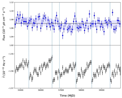
The top and bottom panels in Fig. 1 show the flux temporal evolution and first-time derivative of the spin frequency |$\dot{f}$|, respectively; each data point is obtained with the 60-d Fermi-LAT observation. In addition to the previous three events of the state changes reported by Allafort et al. (2013) and Takata et al. (2020; vertical black dashed lines in Fig. 1), we find new state change from LGF/HSD to HGF/LSD around MJD 58910. Prokhorov & Moraghan (2023) also reported the transition to a high-flux state in 2020 June but they did not discuss any changes in the spin-down rate associated with this event and from HGF/LSD to LGF/HSD around MJD 59510. Since we cannot determine a precise onset time of the state change, we indicate an approximate location with the vertical dashed line in Fig. 1. Hereafter, we denote the newly found states as LGF/HSD 3 and HGF/LSD 3, as indicated in Fig. 1.
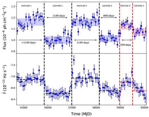
Top: Gamma-ray flux (>0.1 GeV) evolution of PSR J2021+4026 from 2008 to 2023. The shaded region labels the uncertainty of the average flux in different states in 1σ confidence interval. Bottom: The spin-down rate of PSR J2021+4026 from 2008 to 2023. Each point was obtained from the data with a 60-d time bin. The black vertical lines represent the state changes reported in Allafort et al. (2013) and Takata et al. (2020). The lasted two vertical dashed lines indicate new state change reported in this study, and the right-most one is determined by the start of the flux drop. The horizontal dashed lines indicate the averaged spin-down rate for each state.
As Fig. 1 indicates, the time durations of LGF/HSD 2 and HGF/LSD 3 are shorter than those in the previous states. For example, LGF/HSD 2 continues about 840 d, which is significantly shorter than about 1140 d (>1140 d) for HGF/LSD 2 (HGF/LSD 1). We also find that the average flux of the new state is different from the previous values. The flux |$\sim 1.12(1)\times 10^{-6}\, {\rm photon~cm^{-2}~s^{-1}}$| of new HGF/LSD 3 is slightly smaller than |$1.15-1.16\times 10^{-6}\, {\rm photon~cm^{-2}~s^{-1}}$| of the previous HGF/LSD 1 and 2. The flux level of new LGF/HSD 3 is higher than that in the previous two states of LGF/HSD 1 and 2. The flux changes from HGF/LSD to LGF/HSD in previous two events were ∼12–14 per cent (ref. Table 1), while the fractional flux change of the new event is only ∼4 per cent.
Information of the average flux and the parameters of the pulsed structure for PSR J2021+4026.
| 2011 | 2018 | 2021 | ||||
|---|---|---|---|---|---|---|
| HGF/LSD 1c | LGF/HSD 1d | HGF/LSD 2e | LGF/HSD 2f | HGF/LSD 3 | LGF/HSD 3 | |
| MJD | <55850 | 55850–56990 | 56990–58130 | 58130–58970 | 58970–59510 | >59510 |
| Flux1 | 1.16(1) | 0.99(1) | 1.15(1) | 1.01(1) | 1.12(1) | 1.07(1) |
| |$\triangle F_a^2$| | 0.07(1) | 0.10(1) | 0.06(1) | 0.08(1) | 0.03(1) | 0.02(1) |
| |$\triangle F_p^3$| | 14(1) | 16(1) | 12(1) | 11(1) | 4(1) | |
| |$\dot{f}$| | −7.70(4) | −8.17(4) | −7.63(4) | −8.14(4) | −7.81(5) | −8.13(5) |
| pulse 1a | 0.19(2) | 0.13(2) | 0.19(2) | 0.11(2) | 0.16(3) | 0.16(1) |
| pulse 2a | 0.176(7) | 0.174(6) | 0.15(1) | 0.16(1) | 0.164(1) | 0.18(3) |
| pulse 1/pulse 2b | 0.54(6) | 0.24(3) | 0.494(9) | 0.26(1) | 0.41(1) | 0.33(1) |
Notes. 1Average flux in each state (|$10^{-6}\, {\rm photon~cm^{-2}~s^{-1}}$|).
Difference between the average flux of each state and averaged flux of whole data (|$10^{-6}\, {\rm photon~cm^{-2}~s^{-1}}$|).
Flux change from previous state (per cent).
aFWHM.
bRatio of amplitude.
cAllafort et al. (2013), three-Gaussian components.
dAllafort et al. (2013), two-Gaussian components.
eZhao et al. (2017), two-Gaussian components.
fTakata et al. (2020), two-Gaussian components.
A sudden change of the first-time derivative of the frequency, |$\dot{f}$|, with a time-scale of <10 d was observed at the previous state changes from HGF/LSD to LGF/HSD (Allafort et al. 2013; Takata et al. 2020). For new event from HGF/LSD 3 to LGF/HSD 3, on the other hand, a sudden change in timing behaviour could not be confirmed, and the |$\dot{f}$| shows a more gradual evolution to HSD as indicated in the bottom panel of Fig. 1. We obtained the spin-down rate at each point with the data of a 60-d time bin. Neglecting high-order timing noise, we describe the evolution of timing solution using a linear expression as |$f(t)=f(t_0)+\dot{f}(t_0)(t-t_0)$|, where f and |$\dot{f}$| are spin frequency and frequency derivative, respectively. The middle point of each 60-d time bin is chosen to determine the reference time (t0), the uncertainty is determined from the Fourier width, 1/70 d, and the best frequency and spin-down rate in each bin are determined by the results to gain the most significant detections using H-test (de Jager & Büsching 2010). In order to examine the track of the long-term behaviour, we calculate the average time derivatives for each state (i.e. horizontal dashed lines in the bottom panel of Fig. 1). We find that the average value of |$\dot{f}=-7.81(5)\times 10^{-13}~{\rm Hz~s^{-1}}$| in new HGF/LSD 3 is smaller than those in previous HGF/LSD states, while |$\dot{f}=-8.13(5)\times 10^{-13}~{\rm Hz~s^{-1}}$| in new LGF/HSD 3 is consistent with the previous LGF/HSD states within errors.
Fig. 2 summarizes the evolution of the spin frequency from HGF/LSD 3 to LGF/HSD 3. The spin-down rate at each point is calculated with the data of a 70-d time bin, and the starting time difference between two neighbour points is 10 d; namely, two neighbour points overlap the 60-d data. In this figure, we can see a dramatic change of the spin-down rate at around MJD 59510–59600. With the current uncertainty of the data, on the other hand, we cannot confirm the existence of a glitch. If there were a glitch, the frequency jump would be smaller than △f < 10−7 Hz, which is consistent with the previous events from HGF/LSD to LGF/HSD (Allafort et al. 2013; Takata et al. 2020).
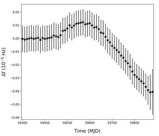
Difference between the observed frequency and predicted frequency from the ephemeris (|$\dot{f}$|, in the last second column (HGF/LSD 3) in Table A1) around MJD 59510. The observed frequency is determined with the data of the 70-d time bin, and two neighbour points overlap the 60-d data. The uncertainty is determined from the Fourier width, 1/70 d.
3.1.2 Time-scale of state change
In this section, we investigate the correlation between the spin-down rate and the gamma-ray flux of PSR J2021+4026 from 2008 to 2023 by utilizing the discrete correlation function (DCF). The DCF measures correlation functions without interpolating in the temporal domain (Edelson & Krolik 1988). The unbinned DCF is defined as
where ai and bj represent the data lists of gamma-ray flux and spin-down rate, respectively, in each time bin of Fig. 1, and |$\overline{a}$| and |$\overline{b}$| represent the average values of the ai and bj, respectively. In addition, σa and σb are the standard errors of a and b, respectively. We calculate the time-lag of each pair (ai, bj) and create the group of the pairs for every 107 s of the time-lag (0 < △t1 < 107 s, 107 s < △t2 < 2 × 10⁷ s,...). For each bin of the time-lag, we obtain number of the pairs, M, and calculate the average of UDCF,
where a standard error for the DCF is defined as
In Fig. 3, we present the DCF curve, which exhibits the maximum correlation coefficient of ∼ 0.32 at a time-lag of 0 s. This indicates that the derivative of frequency changes its state simultaneously with the LAT flux state. The values of the DCF show periodicity with a period of 2 × 10⁸ s, which is approximately 6.5 yr. This result is consistent with that of Takata et al. (2020), which suggests that the time interval between the starting of a specific HGF/LSD is about 6–7 yr.
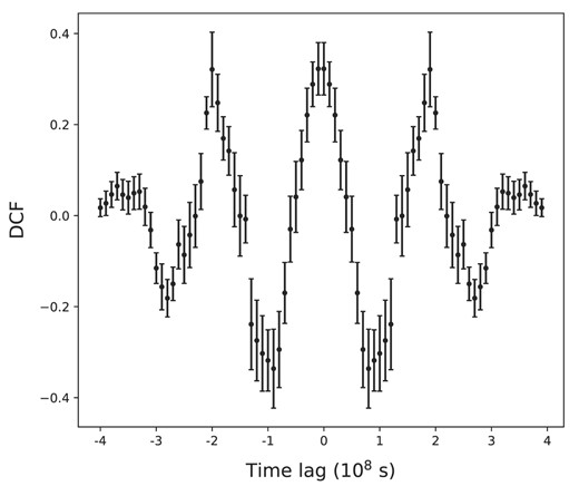
The correlation of Fermi-LAT flux and spin down rate of PSR J2021+4026. The data are from Fermi-LAT in the time range of 2008 to 2023.
3.1.3 Phase-averaged spectrum and pulse profile
In Fig. 4, we present the observed spectra for the new HGF/LSD 3 (black dots) and LGF/HSD 3 (black stars) states. The solid and dotted lines show the fitting function using equation (1). Table 2 summarizes the parameters of the best-fitting function. As indicated by the timing evolution (Fig. 1 and Table 1), the flux change from HGF/LSD 3 to LGF/HSD 3 is only |$\sim 4~{{\ \rm per\ cent}}$|, which is much smaller than 12–14 per cent of the previous two events. The previous state changes from HGF/LSD to LGF/HSD make the spectrum softer; an increase of γ1 and a decrease of the cut-off energy were observed. From the HGF/LSD 3 to LGF/HSD 3, both the power-law index γ1 and the cut-off energy increase.
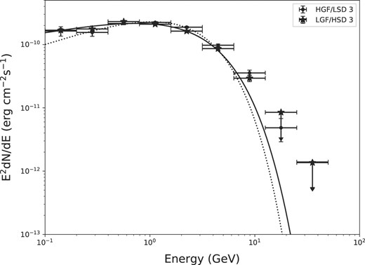
The comparison of spectra at the state of HGF/LSD 3 (dots) and LGF/HSD 3 (stars). The solid line (LGF/HSD 3) and the dotted lines ( HGF/LSD 3) show the best-fitting models for each spectrum according to the ‘PLSuperExpCutoff2’ model (see equation 1).
Parameters of phase-averaged spectra for PSR J2021+4026 in two new states.
| HGF/LSD 3 | LGF/HSD 3 | |
|---|---|---|
| Fluxa | 1.74(1) | 1.69(1) |
| γ1 | 1.60(3) | 1.74(4) |
| Ecut-off (GeV) | 2.2(5) | 2.4(2) |
| HGF/LSD 3 | LGF/HSD 3 | |
|---|---|---|
| Fluxa | 1.74(1) | 1.69(1) |
| γ1 | 1.60(3) | 1.74(4) |
| Ecut-off (GeV) | 2.2(5) | 2.4(2) |
Note. aEnergy flux of each state in units of |$10^{-10}\, {\rm erg~cm^{-2}~s^{-1}}$|.
To investigate the changes in the pulse profile after each state change, we accumulated photons of each new state to derive a global ephemeris for HGF/LSD 3 and LGF/HSD 3 (Table A1), and then folded the corresponding pulse profiles (as shown in Fig. 5). We fit the obtained pulse profiles with two Gaussian functions. Table 1 summarizes the parameters of the fitting functions for each state. In the previous state changes from HSG/LSD state to LGF/HSD, the ratio of height for the first pulse (small pulse) to the height of the second pulse (main pulse) decreased from about 50 per cent to 25 per cent, as Table 1 indicates. From HGF/LSD 3 to LGF/HSD 3, we can see a decrease in the ratio of the pulse height, but the magnitude of the change is smaller that in the previous cases. This would be consistent with the smaller flux change in the new event compared to the previous cases.
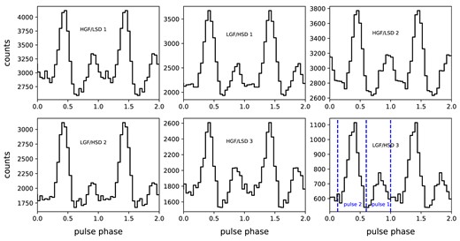
The comparison of the pulse profile for PSR J2021+4026 at the time of HGF/LSD 1, LGF/HSD 1, HGF/LSD 2, LGF/HSD 2, HGF/LSD 3, and LGF/HSD 3. The pulse profile is generated with photon energy >0.1 GeV. The vertical dotted lines show the phase interval of pulse 1 and pulse 2.
3.2 Vela pulsar
3.2.1 Long-term behaviours
After the launch of the Fermi telescope, six glitches of the Vela pulsar have been observed. We search for the semipermanent state changes of the GeV emission triggered by glitches. Fig. 6 presents the evolution of the spin-down rate and the gamma-ray flux of the Vela pulsar. We divide the entire Fermi-LAT data into seven time intervals, which are bounded by the time of the glitches. The top panel of Fig. 6 shows the temporal evolution of the gamma-ray flux, and the bottom panel shows the evolution of the spin-down rate. Timing ephemeris and the emission properties for each inter-glitch interval are summarized in Tables A2 and 3, respectively.
Evolution of gamma-ray flux (top) and spin-down rate (bottom) of the Vela pulsar. The top panel shows the evolution of gamma-ray flux with a 60-d time bin. The black horizontal line shows the average of flux, the vertical lines indicate each glitch epoch, these glitch epochs are derived from the glitch table (see footnote 1). The shaded region labels the uncertainty of the average flux in each inter-glitch interval in 1σ confidence interval. The bottom panel shows the evolution of spin-down rate, and each data set is obtained from the Fermi telescope with a 40-d time bin.
Parameters of spectra of the Vela pulsar at different inter-glitch intervals.
| Time range (MJD) | 54686–55205 | 55422–56500 | 56600–56915 | 56925–57730 | 57740–58510 | 58525–59400 | 59430–59900 |
|---|---|---|---|---|---|---|---|
| Fluxav | 1.077(8) | 1.074(8) | 1.071(8) | 1.063(8) | 1.066(7) | 1.070(8) | 1.070(7) |
| Flux1 | 9.40(2) | 9.49(1) | 9.37(3) | 9.35(2) | 9.4(1) | 9.39(1) | 9.25(2) |
| γ1 | 1.20(1) | 1.205(8) | 1.20(1) | 1.206(8) | 1.214(9) | 1.209(7) | 1.20(1) |
| a | 0.0479(6) | 0.0484(4) | 0.0485(7) | 0.0484(4) | 0.0476(5) | 0.0477(4) | 0.0475(5) |
| Pulse 1a | 0.022(1) | 0.023(1) | 0.023(1) | 0.024(1) | 0.022(1) | 0.024(2) | 0.022(4) |
| Pulse 2a | 0.028(1) | 0.028(1) | 0.0278(7) | 0.027(1) | 0.029(3) | 0.0264(8) | 0.0245(8) |
| Pulse 2/pulse 1b | 0.80(8) | 0.73(7) | 0.71(5) | 0.72(6) | 0.7(1) | 0.68(6) | 0.6(1) |
Notes. av Average flux in each state (10−6 photon cm−2 s−1).
Energy flux of each state in units of 10−8 erg cm−2 s−1.
aFWHM.
bRatio of amplitude.
Despite the frequent glitches of the Vela pulsar, we do not confirm any significant state change in the spectral properties associated with the glitch. In the bottom panel of Fig. 6, the flux shows a small fluctuation with an amplitude of several percentages. However, such a fluctuation can be explained by the random fluctuation observed in the data. Table 3 summarizes the information of the time-averaged spectrum for each inter-glitch interval. We can find that the spectral properties of the energy flux, the spectral index (γ1), and the cut-off energy in the different time intervals are consistent with each other within a limited percentage of errors.
In Fig. 6, we determine the average flux with the 1σ uncertainty for each inter-glitch interval (labelled by the black dashed line and shaded region). Since the flux uncertainties of each inter-glitch interval are encompassed within the range of the long-term average flux, we conclude that there is no significant variation of the flux in different inter-glitch intervals. We also note that one or two data points in each inter-glitch time interval may exhibit notably high or low fluxes, and it is likely caused by random fluctuations. As indicated by Table 3, no significant evolution of spectral properties in different inter-glitch intervals is found.
3.2.2 Pulse profile at different time intervals
The brightness of gamma-ray emission enables us to investigate the temporal evolution of the structure of the pulse profile. In order to explore the long-term evolution trend of the pulsed shape, we accumulate ∼104 photons in the energy range of 0.1–300 GeV to fold a series of pulse profiles using the ephemeris of each inter-glitch interval, as given in Table A2. We employ a fitting approach on the pulse profile using a combination of four Gaussian functions, which can better fit a plateau between two main pulses, as illustrated in Fig. 7. The correlation coefficient of 0.99, derived from the optimal fit employing four Gaussians, surpasses the correlation coefficient of 0.86 obtained when using only three Gaussians to fit the data. With a series of the pulse profiles generated with 104 photons, we then determine the temporal evolution of the phase separation between pulse 1 and pulse 2, the Gaussian width of pulse 1, and the Gaussian width of pulse 2 as shown in Fig. 8. We find that there is no significant semipermanent change shown in the long-term evolution of the pulse profile. The glitch of the Vela may still cause some disturbances of the magnetosphere, as indicated in the radio data (Palfreyman et al. 2018). However, its effect may be on short-term time-scale, or is so small that it is not seen in the gamma-ray emission properties averaged over a time-scale much longer than 10 d.
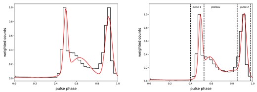
The pulse profile of Vela pulsar (MJD 57740–58510) fitted with 3 (left) and 4 (right) Gaussian functions. The steped lines show the pulse profile with the weighted photons, while the smooth lines depict the results of the Gaussian function fitting. The vertical-dashed-black lines show the phase intervals of pulse 1, pulse 2, and plateau.
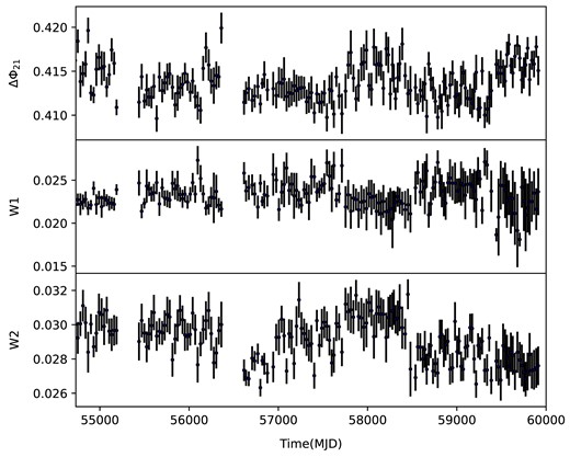
The parameters to describe the pulsed structure in different time intervals of the Vela pulsar. Each data point was determined using at least 10 000 photons. The upper panel shows the phase separation between pulse 1 and pulse 2 (ΔΦ21), respectively, as shown in Fig. 7. The middle and the lower panels show the Gaussian width of pulse 1 and pulse 2 (W1 and W2), respectively. The units of ΔΦ21, W1, and W2 are the phase in one spin cycle.
3.2.3 Searching for >100 GeV photon with Fermi-LAT data
Leung et al. (2014) searched for the pulsed emission above 50 GeV using about 5.2 yr of Fermi-LAT data and reported five photons that probably originated from the Vela pulsar. They also report the highest energy photon about 208 GeV with a significant level of 2.2σ. The results of H.E.S.S.-II (H. E. S. S. Collaboration 2018) also suggest that the spectrum of the pulsed emission from the Vela pulsar extends beyond 100 GeV.
We revisit the search for very high-energy gamma-ray photons with Fermi-LAT data using updated Fermi-LAT gamma-ray catalogue (PASS 8 data), Galactic diffuse emission (gll_iem_v07.fits), and isotropic background emission (P8R3_SOURCE_V3) models, while Leung et al. (2014) used the reprocessed Pass 7 ‘Source’ class (P7REP_SOURCE_V15 IRFs). Following Leung et al. (2014), first, we divide the Fermi-LAT data obtained within MJD 54710–60000 into 50–300 GeV with an ROI (region of interest) of 4° in radius. To select photons originating from the pulsar, we used the gtsrcprob tool to calculate the probability of each photon within ROI associated with the pulsar. We also calculated the probabilities of the photons coming from the Vela X (PPWN) and the Galactic diffuse emission (PGAL). We selected only photons with PVela > max(PPWN, PGAL). Subsequently, the same methodology was applied to each state, utilizing the respective ephemeris obtained from the timing analysis.
Fig. 9 shows the light curve in different energy bands from panel (a) to (c), the panel (d) shows the weighted light curve above 50 GeV. The results in the MJD 54686–56583 in comparison to Leung et al. (2014) are depicted in panel (e) of Fig. 9, which illustrates the energy distribution of photons. We detect seven photons with an energy larger than 50 GeV shown in Table 4. The arrival times of two photons, observed at MJD 56 149 and MJD 56317, are consistent with the results reported by Leung et al. (2014). However, the energy of the photon detected at MJD 56317, ∼54.6 GeV, is significantly smaller than ∼79.5 GeV of the previous result. Although we employ the same method as Leung et al. (2014) to investigate the emission in different time ranges, we do not confirm any photons above 100 GeV.
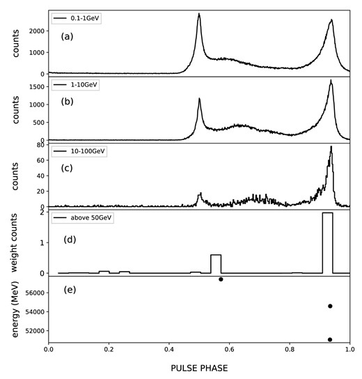
From (a) to (c): the folded light curve in the energy range of 0.1–1, 1–10, and 10–100 GeV using the photons collected within 1° radius centred at the source. From (d) to (e): the weighted light curve in the energy of 50–300 GeV and the energy distribution of the photons above 50 GeV, which are collected within 4° radius and with a source probability of PVela > max(PPWN, PGAL) in the same way as Leung et al. (2014). The data collected during MJD 54686–56583 as an example to find the energy of photons.
Energy, arrival time, and source probability of >50 GeV photons with PPSR large than max(PPWN, PPGAL) for the Vela pulsar.
| Energy (GeV) | Time (MJD) | Pulse phase | PPSR |
|---|---|---|---|
| 51.08 | 55889.11 | 0.93 | 0.98 |
| 57.41 | 56149.28 | 0.57 | 0.59 |
| 54.586 | 56317.21 | 0.93 | 0.98 |
| 51.01 | 57092.19 | 0.91 | 0.81 |
| 87.16 | 57534.33 | 0.81 | 0.68 |
| 50.82 | 58316.77 | 0.90 | 0.89 |
| 67.08 | 59754.76 | 0.92 | 0.97 |
4 DISCUSSION AND SUMMARY
We have investigated the temporal evolution of the characteristics of the GeV emission from two young pulsars, PSR J2021+4026 and the Vela pulsar. For PSR J2021+4026, we confirm new state changes from LGF/HSD to HGF/LSD and from HGF/LSD to LGF/HSD, but the magnitude of the change in the gamma-ray flux and the spin-down rate is smaller than those seen in previous state changes. The pulse shape change is also small compared to previous events. Concerning the state change of the emission and spin-down properties, we speculate that the change of global electric current circulating the magnetosphere could lead to corresponding state change of the emission and spin-down properties, and a larger (smaller) electric current produces larger (smaller) spin-down rate in LGF/HSD (HGF/LSD) state. We expect that the change of gamma-ray flux is due to the change of the size of the particle acceleration/emission regions, and HGF/LSD (LGF/HSD) has a larger (smaller) size of the gap. There is a tendency in the previous states that the HGF/LSD state has a larger cut-off energy in the spectrum and the width of the pulse profile is wider (Takata et al. 2020). This tendency can be understood if the HGF/LSD has a larger acceleration/emission region. Although it is expected that the magnitude of the electric current and the size of the acceleration/emission region are related (Hirotani 2006), a positive or negative correlation will depend on the location of the acceleration/emission region and the geometry of the magnetosphere (Takata et al. 2006). For the most recent state change from HGF/LSD to LGF/HSD, the small change in the spin-down rate implies the change of the electric current is smaller, which results in a small change in the structure of the acceleration/emission region.
Takata et al. (2020) proposed that the crust cracking process triggers the mode change of PSR J2021+4026, and it causes a sudden change in the magnetic field structure of the polar cap region. According to this model, the time-scale between each mode change from HGF/LSD state to LGF/HSD state corresponds to the time-scale to accumulate the magnetic stress inside the crust, and the waiting time-scale in LGF/HSD state is the relaxation time-scale during which the polar cap structure returns to its original state.
Jones (2012) suggested a possible correlation between the neutron star’s spin period and the waiting time-scale of mode change of the transient radio pulsar, and argued the idea of free precession of neutron stars with strained crusts. In this model, the capacity of the acceleration of particles within the magnetosphere was linked to different phases of precession. The precession model has been widely applied to the observed periodic variations of the spin-down rate of PSR B1828−11 (Link & Epstein 2001; Ashton, Jones & Prix 2017). For PSR J2021+4026, we found that the waiting time in LGF/HSD 2 (∼840 d) and HGF/LSDF 3 (∼530 d) were shorter than the previous corresponding states (∼1140 d), indicating that the mode change is quasi-periodic event. Such a quasi-periodicity may be incompatible with the free-precession model, for which the stable periodic variation of the spin-down rate will be expected.
Among the transitioning radio pulsars, PSRs J0738−4042 and B2035+36 have shown a mode change with relatively large variations in the spin-down rate, |$|\Delta \dot{f}|/f\sim 7$| per cent and 12 per cent, respectively. The magnitude of the spin-down rate change of the two pulsars is similar to |$|\Delta \dot{f}|/f\sim 7$| per cent of PSR J2021+4026. Moreover, the waiting time to the next mode change of three pulsars will be of the order of or longer than ∼10 yr; it is observed once or twice mode changes of PSR J0738−4042 over 50 yr (Lower et al. 2023) and once of PSR B2035+36 over 9 yr (Kou et al. 2018). Brook et al. (2014) argued the mode change of PSR J0738−4042 with an asteroid encounter model (Cordes & Shannon 2008). In this model, the asteroid with neutral charge can approach to the pulsar magnetosphere, and it is evaporated and ionized by an X-ray irradiation of the pulsar. The ionized gas that migrates within the magnetosphere changes the torque exerted on the neutron star and the emission properties. Due to the size of the frequency jump and waiting time in several years, the asteroid encounter may be an attractive model as the origin of the mode change of PSR J2021+4026.
Since about 50 glitching Fermi-LAT pulsars have been confirmed (see footnote 1), it is not unexpected that PSR J2021+4026 has experienced the glitch process of the neutron star. In this paper, we focus on the Vela pulsar, which is both a glitching and bright gamma-ray pulsar, we analysed Fermi-LAT data of the Vela pulsar to investigate the influence of glitch on its gamma-ray emission. Palfreyman et al. (2018) reported sudden changes in the radio pulse shape coincident with the 2016 glitch event of Vela pulsar, indicating the glitch affected the structure of the magnetosphere. Bransgrove, Beloborodov & Levin (2020) suggested that the glitch launched the Alfven wave, which subsequently caused the high-energy radiation and the electron–positron pair creation. They suggest that the created pairs quench the radio emission at the 2016 event of the Vela pulsar. Although the enhancement of the gamma-ray flux is expected during propagation of the Alfven wave in the magnetosphere, the predicted time-scale of the existence of the wave, ∼0.2 s, is too short to be investigated with Fermi-LAT data. We also did not find any evidence for the change of the magnetosphere structure for the Vela pulsar in a time-scale of years, as discussed in Section 3.2. Consequently, we cannot conclude that the glitch is the trigger of PSR J2021+4026 based on this study.
In summary, we have examined the evolution of gamma-ray flux and spin-down rate in two bright gamma-ray pulsars, PSR J2021+4026 and the Vela pulsar. We confirmed new states change from LGF/HSD to HGF/LSD and from HGF/LSD to LGF/HSD observed for PSR J2021+4026, occurring around MJD 58 910 and MJD 59510, respectively. We found that the waiting time, the change in the flux and the first time derivative of frequency are smaller than previous events. The change in the shape of the pulse profile is also smaller than those of the previous events. Our results confirm that the state change of PSR J2021+4026 is not regularly repeated but quasi-periodically repeated with the different magnitude of change of the gamma-ray flux and the spin-down rate. We also carried out the timing and spectral analysis of the Vela pulsar to investigate the effect of the glitch on the observed gamma-ray emission properties, since the radio observation indicates that the glitch disturbs the structure of the magnetosphere. However, we did not confirm any significant state change of the gamma-ray emission triggered by the glitch of the Vela pulsar. Finally, using the 15-yr Fermi-LAT data of the Vela pulsar to search photons above 100 GeV, we did not find any photons above 100 GeV from the Fermi-LAT data. We still did not find any evidence for the change of the magnetosphere structure in a time-scale of years in the 2016 glitch, while the created pairs may quench the radio emission.
ACKNOWLEDGEMENTS
We express our appreciation to an anonymous referee for useful comments and suggestions. We appreciate Drs Kisaka and S.Q. Zhou for useful discussion on glitching pulsars. This work made use of data supplied by the LAT data server of the Fermi Science Support Center (FSSC) and the archival data server of NASA’s High Energy Astrophysics Science Archive Research Center (HEASARC). H.H. Wang issupported by the Scientific Research Foundation of Hunan Provincial Education Department (21C0343). J. Takata is supported by National Key Research and Development Program of China (2020YFC2201400) and the National Natural Science Foundation of China (grant no. 12173014). Lupin C.-C. Lin is supported by NSTC through grants 110-2112-M-006-006-MY3 and 112-2811-M-006-019. H.H. Wang and P.H. Tam are supported by the National Natural Science Foundation of China (NSFC) grant 12273122 and a science research grant from the China Manned Space Project (no. CMS-CSST-2021-B11).
DATA AVAILABILITY
The Fermi-LAT data used in this article are available in the LAT data server at https://fermi.gsfc.nasa.gov/ssc/data/ access/.
The Fermi-LAT data analysis software is available at https://fermi.gsfc.nasa.gov/ssc/data/analysis/software/.
We agree to share data derived in this article on reasonable request to the corresponding author.
Footnotes
References
APPENDIX A: EPHEMERIS OF PSR J2021+4026 AND VELA PULSAR
We performed the timing analysis in HGF/LSD 3 and LGF/HSD 3 of PSR J2021+4026 and each state of Vela pulsar. We use the Gaussian kernel density estimation method to build an initial template. We then use this template to cross-correlate with the unbinned geocentred data to determine the pulse TOA for each pulse. We then fitted the TOAs according to a timing model to obtain the spin frequency, spin-down rate, and other parameters. In order to further investigate the emission behaviour between different states, we extract the source events within a 1° radius centred at the target. As shown in Tables A1 and A2, ephemeris of each state are obtained to compare the shapes of pulse profile of each state.
Ephemerides of PSR J2021+4026 derived from LAT Data covering MJD 54710–60000.
| Parameters | ||||||
|---|---|---|---|---|---|---|
| Right ascension | 20:21:29.99 | |||||
| Declination | +40:26:45.13 | |||||
| Valid MJD range | 54710–55850 | 55850–56980 | 56990–58130 | 58140–58900 | 58920–59500 | 59550–60000 |
| Pulse frequency, f(s−1) | 3.769066845(7) | 3.768952744(6) | 3.768891254(7) | 3.768823695(3) | 3.768775022(1) | 3.768734495(7) |
| First derivative,|$\dot{f}(10^{-13} s^{-2})$| | −7.762(1) | −8.206(1) | −7.699(1) | −8.132(1) | −7.822(4) | −8.173(3) |
| Second derivative,|$\ddot{f}(10^{-21} s^{-3})$| | 0.51(3) | 0.56(2) | −0.12(1) | 1.98(3) | 2.19(1) | −13.2(1) |
| Third derivative,|$\dddot{f}(10^{-28} s^{-4})$| | −0.33(4) | 69.3(3) | −0.31(4) | 3.6(1) | 0.4(2) | 169(6) |
| Fourth derivative,f(4)(10−35s−5) | −0.11(1) | −1.14(7) | 0.38(5) | −8.3(3) | −5.6(8) | −94(2) |
| Fifth derivative,f(5)(10−41s−6) | 0.13(3) | −0.22(1) | 0.058(1) | −1.26(9) | 0.3(1)1 | 281(9) |
| Sixth derivative,f(6)(10−48s−7) | −0.26(5) | 0.11(1) | −0.08(1) | 2.9(3) | −1.8(4) | −316(9) |
| Seventh derivative, f(7)(10−55 s−8) | 0.23(3) | 0.51(3) | −0.06(1) | 2.8(6) | ⋅⋅⋅ | 51(9) |
| Eighth derivative, f(8)(10−62 s−9) | −0.08(1) | 0.33(2) | 0.10(2) | −9(2) | ⋅⋅⋅ | 210(3) |
| Epoch zero (MJD) | 54936 | 56600 | 57500 | 58500 | 59200 | 59800 |
| Time system | TDB(DE405) | |||||
The ephemerides of Vela before and after each glitch.
| Parameters | |||||||
|---|---|---|---|---|---|---|---|
| Right ascension | 08:35:20.6033089 | ||||||
| Declination | −45:10:34.82304 | ||||||
| Valid MJD range | 54686–55205 | 55422–56500 | 56600–56915 | 56925–57730 | 57740–58510 | 58525–59400 | 59430-59900 |
| Spin frequency, f(s−1) | 11.19025957434(1) | 11.189275117(8) | 11.18782702(7) | 11.186479678(1) | 11.1860906325(4) | 11.18531013(1) | 11.18411112(1) |
| First derivative, |$\dot{f}(10^{-11}$| s−2) | −1.55759513(7) | −1.56292(1) | −1.5614(4) | −1.55703(1) | −1.561418(2) | −1.56366(8) | −1.5633(1) |
| Second derivative, |$\ddot{f}(10^{-21}$| s−3) | 0.791(2) | 1.88(3) | 21(2) | 0.86(1) | 1.690(7) | −1.56366(8) | −6.6(6) |
| Third derivative, |$\dddot{f}(10^{-28}$| s−4 | −0.7509(3) | 0.17(1) | −16(2) | 0.091(4) | −0.202(7) | −3.1(4) | 0.60(6) |
| Fourth derivative, f(4)(10−34 s−5) | 0.042(3) | −0.13(9) | −6.9(1) | ⋅⋅⋅ | ⋅⋅⋅ | 2.9(4) | 5.2(4) |
| Fifth derivative, f(5)(10−41 s−6) | 0.481(1) | −0.15(8) | 13(2) | ⋅⋅⋅ | ⋅⋅⋅ | −6.6(1) | −0.10(1) |
| Sixth derivative, f(6)(10−48 s−7) | −0.26(4) | 0.7(1) | −5.4(1) | ⋅⋅⋅ | ⋅⋅⋅ | 7(1) | 6.7(8) |
| Seventh derivative, f(7)(10−55 s−8) | −2.71(5) | −0.9(2) | ⋅⋅⋅ | ⋅⋅⋅ | ⋅⋅⋅ | −5.1(9) | ⋅⋅⋅ |
| Eighth derivative, f(8)(10−63 s−9) | −1.2(2) | 4(1) | ⋅⋅⋅ | ⋅⋅⋅ | ⋅⋅⋅ | 14(2) | ⋅⋅⋅ |
| Epoch zero (MJD) | 54853 | 55600 | 56700 | 57700 | 58000 | 58600 | 59500 |
| Time system | TDB(DE405) | ||||||
Note. The numbers in parentheses denote 1σ errors in the last digit.
