


ABSTRACT
We propose an efficient and robust method to estimate the halo concentration based on the first moment of the density distribution, which is |$R_1\equiv \int _0^{r_{\rm vir}}4\pi r^3\rho (r)\mathrm{ d}r/M_{\rm vir}/r_{\rm vir}$|. We find that R1 has a monotonic relation with the concentration parameter of the Navarro–Frenk–White (NFW) profile, and that a cubic polynomial function can fit the relation with an error |$\lesssim 3~{{\ \rm per\ cent}}$|. Tests on ideal NFW haloes show that the conventional NFW profile fitting method and the Vmax/Vvir method produce biased halo concentration estimation by |$\approx 10~{{\ \rm per\ cent}}$| and |$\approx 30~{{\ \rm per\ cent}}$|, respectively, for haloes with 100 particles. In contrast, the systematic error for our R1 method is smaller than 0.5 per cent even for haloes containing only 100 particles. Convergence tests on realistic haloes in N-body simulations show that the NFW profile fitting method underestimates the concentration parameter for haloes with ≲300 particles by |$\gtrsim 20~{{\ \rm per\ cent}}$|, while the error for the R1 method is |$\lesssim 8~{{\ \rm per\ cent}}$|. We also show other applications of R1, including estimating Vmax and the Einasto concentration ce ≡ rvir/r−2. The calculation of R1 is efficient and robust, and we recommend including it as one of the halo properties in halo catalogues of cosmological simulations.
1 INTRODUCTION
Dark matter haloes, as the building blocks of the cosmic structures in our Universe, are virialized objects formed by gravitational instability. The assembly of haloes proceeds hierarchically, where small haloes are formed early and merge with each other to form larger ones. The assembly history of dark matter haloes correlates strongly to the halo structure, and many semi-analytical models have been proposed to explain this correlation and to predict halo structure from its assembly history (e.g. Navarro, Frenk & White 1997; Wechsler et al. 2002; Zhao et al. 2003a, 2009; Lu et al. 2006; Correa et al. 2015; Diemer & Joyce 2019). In addition, galaxies are born in the centres of dark matter haloes and evolve following the halo assembly process (see Mo, Van den Bosch & White 2010, for a review), so that dark matter haloes and galaxies are tightly related to each other. This motivates many attempts to model the galaxy–halo connection to understand galaxy formation and evolution (see Baugh 2006; Mo, Van den Bosch & White 2010; Wechsler & Tinker 2018, for reviews). Clearly, it is of paramount importance to accurately characterize the structure of dark matter haloes.
Numerical N-body simulations with collisionless cold dark matter particles provide an essential tool to study the structure of dark matter haloes. To begin with, dark matter haloes are identified with a halo-finding algorithm, such as the Friends-of-Friends (FoF) algorithm (e.g. Huchra & Geller 1982; Davis et al. 1985). Based on the spherical collapse model, a dark matter halo is defined as the collection of particles within a radius within which the mean density reaches some chosen value. This radius is usually referred to as the virial radius, rvir, and the total mass enclosed is the halo mass, Mvir. The radial density profiles of dark matter haloes are found to be well described by the universal Navarro–Frenk–White (NFW) function,
specified by the two free parameters, rs and ρ0, or equivalently, Mvir and the halo concentration, c ≡ rvir/rs (Navarro, Frenk & White 1997).
However, the determination of the concentration parameter for simulated haloes is not straightforward. Many methods have been used to estimate the concentration parameters of simulated haloes from the spatial distribution of dark matter particles (e.g. Jing 2000; Bullock et al. 2001; Klypin et al. 2001; Wechsler et al. 2002; Zhao et al. 2003a, b, 2009; Duffy et al. 2008; Klypin, Trujillo-Gomez & Primack 2011; Klypin et al. 2016). One approach is to sample the radial density distribution of simulated haloes in discrete bins and fit it with the NFW profile (e.g. Bhattacharya et al. 2013). This method has several shortcomings. First, the estimated concentration is subject to the choice of discrete bins. The use of large bin sizes tends to smooth the gradient of the radial profile and cause an underestimate of the halo concentration, while the use of too small bins can introduce too much noise. In general, it is difficult to find an optimal binning strategy, particularly when a halo is only sparsely sampled. Secondly, the fitting method relies on the prior choice of the halo profile, which is the NFW profile in this case. Therefore, any deviations from the NFW profile will make the output concentration biased (Einasto 1965; Navarro et al. 2004; Wang et al. 2020b). Finally, the fitting procedure is relatively time-consuming, making it difficult to do for the large number of haloes found in large cosmological simulations.
To overcome some of the issues in the NFW profile fitting, other estimators of halo concentration have been proposed. One example is the method based on Vmax/Vvir (Klypin et al. 2001, 2016; Klypin, Trujillo-Gomez & Primack 2011; Prada et al. 2012), where |$V_{\rm max}=\tt {MAX}(\sqrt{GM(\lt r)/r})$| is the maximum of the circular velocity as a function of r, and |$V_{\rm vir}=\sqrt{GM(\lt r_{\rm vir})/r_{\rm vir}}$| is the virial velocity. This quantity is closely related to the halo concentration for an NFW halo. However, this relation is ill-defined for haloes with concentration below 2.16 (Klypin et al. 2001), since by definition Vmax cannot be smaller than Vvir. The halo concentration can also be inferred from rf/rvir, where rf is the radius within which the mass is fMvir, with 0 < f < 1 (e.g. Lang, Holley-Bockelmann & Sinha 2015). In addition, there are also methods based on the integrated mass profile (Poveda-Ruiz, Forero-Romero & Muñoz-Cuartas 2016) and the Voronoi Tessellation (Lang, Holley-Bockelmann & Sinha 2015).
In this paper, we propose an efficient and robust method to estimate the concentration parameter of NFW haloes based on the first moment of the density distribution. Section 2 introduces the data we use in this study. Section 3 introduces three different methods to estimate the halo concentration, and we test their performance in Section 4. Section 5 shows the mass–concentration relation obtained from the ELUCID simulation, to demonstrate the application of our method to large cosmological simulations. Section 6 discusses other applications of R1, including estimating Vmax of haloes and the Einasto concentration parameter. Finally, Section 7 summarizes our main results. Throughout this paper, we use ‘log’ to denote 10-based logarithm.
2 DATA
The estimation of halo concentration is subject to the sampling effect, where low-mass haloes are poorly sampled in N-body simulations, and the force softening effect, which can smooth the density profile in the inner region and cause an underestimation of the halo concentration (e.g. Power et al. 2003; Ludlow, Schaye & Bower 2019; Mansfield & Avestruz 2021). To separate the impact of these two effects, we use two different data sets to test the performances of different methods: ideal haloes generated from NFW profiles with different halo parameters, and realistic haloes selected from N-body simulations of different resolutions and force softening lengths. We also apply our method to a large N-body simulation to demonstrate its capability of recovering halo concentrations in large cosmological simulations.
2.1 Ideal NFW haloes
We generate ideal NFW haloes using the halofactory package based on Eddington’s inversion method (see appendix A for details). Here we use haloes with four different concentrations, c = 1, 5, 10, and 20, a range sufficient to cover haloes in cosmological N-body simulations. For each concentration, we generate individual haloes using different numbers of particles, ranging from ∼100 to ≳104, to test the robustness of a given concentration estimator. For a given particle number, we use 10 000 random realizations to evaluate the statistical uncertainties.
2.2 N-body simulations
2.2.1 IllustrisTNG-Dark
The IllustrisTNG project consists of several dark-matter-only and hydrodynamical simulations (Pillepich et al. 2018; Nelson et al. 2019). Here we use the dark-matter-only simulations with different resolutions and gravitational softening lengths to test the impact on the concentration estimation. The information of these simulations is summarized in Table 1 (Nelson et al. 2019). It is noteworthy that TNG100-1-Dark and TNG100-3-Dark have identical initial conditions, but different mass resolutions and gravitational softening lengths. The IllustrisTNG project was based on a cosmology consistent with the results in Planck Collaboration XIII (2016), where |$\Omega _\Lambda =0.6911$|, Ωm = 0.3089, σ8 = 0.8159, ns = 0.9667, and h = 0.6774. Dark matter haloes are identified using the FoF algorithm with a linking length that is 0.2 times the mean inter-particle distance (Davis et al. 1985), and their masses are assigned as the total dark matter mass enclosed within the aperture where the mean overdensity is 200 times the critical density. This mass is denoted as M200c, and the corresponding radius and concentration are denoted as r200c and c200c, respectively. The halo centre is specified as the location of the particle with the minimal gravitational potential. Substructures are identified with the subfind algorithm (Springel et al. 2001).
Summary of the N-body simulations used in this study.
| Simulation | Lbox[h−1 Mpc] | Particle number | Particle mass [h−1 M⊙] | Gravitational softening length [h−1 kpc] |
|---|---|---|---|---|
| TNG50-1-Dark | 35 | 21603 | 3.7 × 10⁵ | 0.2 |
| TNG100-1-Dark | 75 | 18203 | 6.0 × 10⁶ | 0.5 |
| TNG100-3-Dark | 75 | 4553 | 3.8 × 10⁸ | 2.0 |
| ELUCID | 500 | 30723 | 3.1 × 10⁸ | 3.5 |
2.2.2 ELUCID
The ELUCID1 simulation (Wang et al. 2013, 2014, 2016; Tweed et al. 2017) is a constrained simulation, run with a memory-optimized version of gadget-2 (Springel et al. 2005) known as l-gadget, to reconstruct the density field and formation history of our local Universe based on the Sloan Digital Sky Survey DR7 (York et al. 2000). It is thus one particular realization of the structure formation model in question. This simulation has 30723 dark matter particles, each with a mass of |$3.09\times 10^8h^{-1}\rm M_\odot$|, in a box with a side length of |$500h^{-1}\rm Mpc$|. This simulation assumes a Lambda cold dark matter cosmology with Ωm = 0.258, |$\Omega _\Lambda =0.742$|, σ8 = 0.80, ns = 0.96, and h = 0.72. The information of the ELUCID simulation is summarized in Table 1 (Wang et al. 2016). ELUCID uses the same procedure as IllustrisTNG to identify and define dark matter haloes (see Section 2.2.1). The large volume and relatively high resolution of the ELUCID simulation allow us to investigate the mass–concentration relation over a large halo mass range.
3 METHOD
Here we introduce three methods to estimate halo concentration: two commonly used methods and our R1 method. In addition, three other methods are discussed in Appendix C together with their performance on ideal NFW haloes.
3.1 The R1 method
The total mass of a dark matter halo is expressed as
Here ρ(r) is the radial density profile and rvir is the halo radius, which is usually defined as the radius within which the enclosed mean density just exceeds some chosen value. The dimensionless first moment of the density distribution, R1, can be defined as
which can be expressed analytically for an NFW profile as
Despite the complicated functional form, the relation between R1 and c is actually quite simple, as shown in Fig. 1. We fit both R1(c) and c(R1) with third-order polynomial functions:
The bottom panels of Fig. 1 show the fractional difference between the relation in equation (4) and the fitting formula of equation (5). The fractional deviation is |$\lesssim 0.1~{{\ \rm per\ cent}}$| for the R1–c relation and |$\lesssim 3~{{\ \rm per\ cent}}$| for the c–R1 relation. We note that the relation between R1 and c depends neither on cosmology nor on the threshold density chosen to define dark matter haloes.
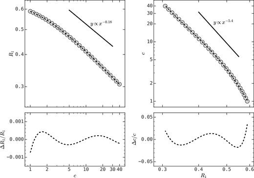
The relation between c and R1 for an NFW profile. Top panels: the circles are the analytical results obtained through equation (4), and the dashed lines are the fitted third-order polynomial functions in equation (5). Bottom panels: the fractional difference between the relation in equation (4) and the third-order polynomial fits.
3.2 The NFW profile fitting method
The halo concentration can also be estimated by fitting the density distribution with an NFW profile (e.g. Bhattacharya et al. 2013). One can start with the cumulative mass distribution for an NFW halo:
where
The optimal concentration can be found by minimizing the χ2 defined as
where Mi = M(< ri) − M(< ri − 1) is the mass within the i-th radial bin according to the NFW profile, |$M_i^{\rm sim}$| is the total mass of particles in the same radial bin for the simulated halo, and ni is the number of particles in that bin. Here we take 20 equally spaced radial bins from 0.01rvir to rvir on the logarithmic scale. Clearly, the result of the NFW profile fitting method is subject to the choice of binning. In Appendix B, we test the performance with three different binning strategies and adopt the best one here to compare with the other two methods.
3.3 The Vmax/Vvir method
For NFW haloes, the concentration parameter is also related to the ratio between the maximum circular velocity and the virial velocity,
where |$V_{\rm circ}(r) = \sqrt{GM(\lt r)/r}$|, and the relation is
(e.g. Klypin et al. 2001). Note that this relation is only applicable for c ≳ 2.16 since Vmax ≥ Vvir by definition.
4 TESTING THE PERFORMANCE OF THE HALO CONCENTRATION ESTIMATORS
4.1 Tests on ideal NFW profile
We first test the performance of the three concentration estimation methods on ideal NFW haloes generated from the halofactory package (see Appendix A). The results are presented in Fig. 2. The four columns are for four different input halo concentrations, from c = 1 to c = 20, and the three rows present the results for three different methods. In each panel, the red solid line shows the median fractional deviation of the concentration parameter estimated from 10 000 halo realizations as a function of particle number, and the magenta dashed lines and the cyan dotted lines show the 16th–84th and 2.5th–97.5th percentile ranges, respectively.
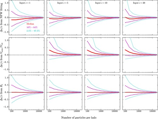
The fractional difference between the input and the estimated concentrations with the NFW fitting method (top panels), the Vmax/Vvir method (middle panels), and the R1 method (bottom panels) for ideal NFW haloes generated with halofactory as a function of the number of particles in the halo. The red solid, magenta dashed, and cyan dotted lines show the 50th, 16th–84th, and 2.5th–97.5th percentiles. This figure shows that the R1 method gives an unbiased and less uncertain estimation of the input halo concentration compared with the other two methods. The middle left panel is empty since the Vmax/Vvir method cannot be applied to haloes with c < 2.16.
First, when the particle number is sufficiently large (≳104), all three methods perform equally well and the fractional deviation of the halo concentration estimation for 95 per cent of halo realizations is within |$\pm 5~{{\ \rm per\ cent}}$|. Secondly, when the particle number decreases to a few hundred, the NFW profile fitting method tends to underestimate halo concentration by |$\approx 10~{{\ \rm per\ cent}}$|. We note that this result is subject to the choice of binning (see Appendix B). The Vmax/Vvir method tends to overestimate the halo concentration by |$\approx 30~{{\ \rm per\ cent}}$|, which was already noted in previous studies (see Poveda-Ruiz, Forero-Romero & Muñoz-Cuartas 2016). In contrast, the fractional deviation of the median value for our R1 method is less than 0.5 per cent. Thirdly, the distribution of the estimated concentration broadens with decreasing particle numbers. When only 100 particles are used, the width of the 16th–84th percentiles is about 0.76c − 1.03c for the NFW fitting method, 0.91c − 1.06c for the Vmax/Vvir method, and 0.63c − 0.91c for our R1 method. Therefore, the R1 method also yields the smallest variance among all three methods when haloes are poorly sampled. We also note that the Vmax/Vvir method is not applicable to haloes with c ≲ 2.16. In addition, Appendix C presents the performance of three other concentration estimation methods. Our test results show that their performances are poorer than the R1 method, even though some of them are more difficult to obtain from simulation data.
Finally, Appendix D shows the distributions of the logarithmic deviation of halo concentration estimated with our R1 method. These distributions can be described by Gaussian functions, and the scatter decreases with increasing particle number and decreasing input concentration. A fitting function is provided to describe the dependence of the scatter on the particle number and the input concentration (see equation D2).
4.2 Impact of resolution
We have already shown that our R1 method outperforms the other two methods in halo concentration estimation using ideal NFW haloes. However, low-mass haloes in realistic N-body simulations are not only poorly sampled, but also subject to the force softening used to avoid unphysical gravity when two particles are too close to each other (e.g. Power et al. 2003; Ludlow, Schaye & Bower 2019). In addition, haloes in simulations are not spherically symmetric and are not perfectly relaxed (e.g. Jing 2000; Jing & Suto 2002). While it is not a priori clear what the true concentration is for haloes in simulations, we can investigate which method gives the best convergence with the numerical resolution.
Here we use three simulations from the IllustrisTNG suite, which are TNG50-1-Dark, TNG100-1-Dark, and TNG100-3-Dark, to test the impact of numerical resolution on the estimation of halo concentration. Note again that the latter two simulations use identical initial conditions and simulation code, but different mass resolutions and gravitational softening lengths (see Table 1). Fig. 3 shows the mass–concentration relation obtained from these three simulations, and the top and bottom panels show results obtained from the NFW profile fitting method and our R1 method, respectively. First, both methods produce nearly identical median mass–concentration relations and the 16th–84th percentiles in TNG100-1-Dark, whose particle mass is about |$6.0\times 10^6h^{-1}\rm M_\odot$|. Secondly, the NFW profile fitting method underestimates the concentration of |$10^{11}h^{-1}\rm M_\odot$| haloes (≲300 particles) by |$\gtrsim 20~{{\ \rm per\ cent}}$| in TNG100-3-Dark, whose particle mass is about |$3.8\times 10^8h^{-1}\rm M_\odot$|. In contrast, the R1 method yields nearly identical mass–concentration relations across the entire mass range in these two simulations, and the fractional deviation for low-mass haloes is |$\lesssim 8~{{\ \rm per\ cent}}$| between the two simulations. Note that a |$10^{11}h^{-1}\rm M_\odot$| halo in TNG100-3-Dark is represented by only ≲300 particles. Finally, the mass–concentration relations obtained from TNG50-1-Dark by the two methods are similar to each other, and to those obtained from TNG100-1-Dark. The discrepancy at the massive end owes to cosmic variance, since the two simulations have different box sizes and initial conditions. In Appendix G, we show that the concentration parameter c200c can also be obtained from R1 with integrating only to r500c, which is commonly used in observation.
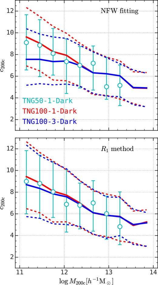
The mass–concentration relation for TNG50-1-Dark (cyan error bars), TNG100-1-Dark (red lines), and TNG100-3-Dark (blue lines), where the 16th–50th–84th percentiles are presented. The upper panel shows the result obtained with the NFW profile fitting method, and the lower panel shows the result obtained with our R1 method. The NFW profile fitting method underestimates halo concentration for low-resolution simulations, while this effect is marginal for our R1 method.
Fig. 4 compares the halo concentration estimated with the NFW profile fitting method and our R1 method in the three TNG-Dark simulations, where the open circles and error bars show the median and the 16th–84th percentiles, respectively. First, both methods yield similar concentrations for massive haloes and low-concentration low-mass haloes. Secondly, the NFW fitting method produces lower concentrations than our R1 method for high-concentration low-mass haloes, and the discrepancy is larger in lower resolution simulations. Combined with the results in Fig. 3, we infer that the NFW profile fitting method tends to underestimate the concentration of high-concentration low-mass haloes in low-resolution simulations for two reasons. The first one is that the NFW profile fitting method tends to underestimate halo concentration for poorly sampled haloes, as shown in Fig. 2, but this effect becomes marginal once more than a few thousand particles are sampled. The second reason is that, for a given simulation volume, the force softening length is larger in lower resolution runs, and so is a larger fraction of the virial radius in lower mass haloes, and therefore has a large impact on the central mass profile. This will consequently cause the underestimation of halo concentration in the NFW profile fitting method. A common strategy to tackle this problem is to exclude particles below the convergence radius during the fitting, where the convergence radius is defined such that the two-body dynamical relaxation time-scale of the particles within this radius is comparable to the age of the universe (Power et al. 2003; Duffy et al. 2008; Correa et al. 2015). However, the convergence radius is about 0.1r200c for haloes with a few hundred particles (Ludlow, Schaye & Bower 2019), and excluding particles within this radius will cause systematic underestimations of the concentration parameter by |$\approx 20~{{\ \rm per\ cent}}\!-\!50~{{\ \rm per\ cent}}$| for haloes with c ≈ 10–20 for the NFW fitting method (see Appendix B). In contrast, the R1 method is less affected by the inclusion, since it gives more weight to the outer region of dark matter haloes.
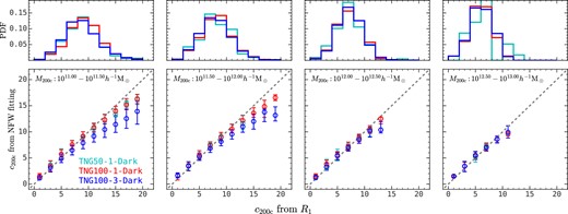
Top panels: the probability distribution function of halo concentration estimated with our R1 method in three TNG-Dark simulations. Bottom panels: comparison of halo concentration estimated from the NFW profile fitting method and our R1 method in different halo mass bins. When combined with Fig. 3, this figure demonstrates that, compared with our R1 method, the NFW fitting method underestimates halo concentration for haloes sampled with small numbers (≲300) of particles, especially for high-concentration haloes.
Finally, there is still a noticeable discrepancy between these two methods for high-concentration haloes with |$M_{\rm 200c}\approx 10^{11}h^{-1}\rm M_\odot$| in TNG100-1-Dark and TNG50-1-Dark, where a |$10^{11}\,h^{-1}\,\rm M_\odot$| halo is well represented by ≳2.7 × 10⁵ particles. In Appendix E, we find that these haloes deviate from the NFW profile due to the stripping of mass in the outskirts, and the mass distribution recovered from both concentrations matches the data equally well, despite the |$\gtrsim 10~{{\ \rm per\ cent}}$| systematics in the values of the estimated concentration. Nevertheless, these haloes constitute only a small portion of all haloes in the given mass bin, as one can see from the histogram in the top panels of Fig. 4.
5 THE MASS–CONCENTRATION RELATION IN THE ELUCID SIMULATION
It has been shown in Section 4 that our R1 method outperforms the conventional method in the halo concentration estimation on both ideal NFW haloes and realistic haloes in N-body simulations, and it can give unbiased estimation of the concentration parameter for haloes with more than 200 particles. For this reason, we apply the R1 method to the ELUCID simulation and infer the mass–concentration relation for haloes with 11 ≲ log (M200c/[h−1M⊙]) ≲ 15. Notably, a |$10^{11}h^{-1}\rm M_\odot$| halo is only represented by about 300 particles in ELUCID.
Fig. 5 shows the median mass–concentration relation in ELUCID, as well as the 16th–84th percentiles. Here relaxed and unrelaxed haloes are separated according to the criterion in Neto et al. (2007), which is
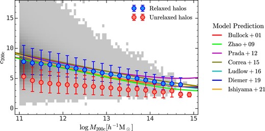
The mass–concentration relation in the ELUCID simulation for relaxed (blue error bars) and unrelaxed (red error bars) haloes, and the 16th–84th percentiles. The grey colour scale encodes the number density of dark matter haloes. The criterion for separating relaxed and unrelaxed haloes is shown in equation (11). The solid lines are the predictions of different semi-analytical models: Bullock + 01 (Bullock et al. 2001), Zhao + 09 (Zhao et al. 2009), Prada + 12 (Prada et al. 2012), Correa + 15 (Correa et al. 2015), Ludlow + 16 (Ludlow et al. 2016), Diemer + 19 (Diemer & Joyce 2019), and Ishiyama + 21 (Ishiyama et al. 2021).
where rmin-pot is the position of the particle with the minimal gravitational potential, and rcom is the centre of mass of all dark matter particles within r200c. Note that Neto et al. (2007) use two additional conditions to select haloes in equilibrium. They require that the mass fraction in substructures is lower than a threshold value and that the ratio between the kinetic energy and the potential energy is lower than a threshold. Here we use only the criterion in equation (11), for three reasons. First, as shown in Neto et al. (2007), equation (11) alone can select most of the haloes in equilibrium (see their fig. 2). Secondly, equation (11) is the simplest criterion to implement in N-body simulations, whereas the other two criteria require either identifying substructures or calculating the gravitational potential for each particle. Thirdly, the other two criteria suffer from some ambiguities. For instance, the substructure mass fraction is subject to the substructure finder used (e.g. van den Bosch & Jiang 2016) and to the resolution of the simulation (e.g. van den Bosch et al. 2018). Besides, the exact value of the virial ratio for selecting haloes in equilibrium is still under debate, as many argued that the surface pressure and even the non-spherical shape of haloes should be taken into account (e.g. Davis, D’Aloisio & Natarajan 2011; Klypin et al. 2016). Here one can see that the concentration parameter decreases from ≈8 to ≈4 with increasing mass for relaxed haloes, and from ≈4 to ≈2 for unrelaxed ones. It has already been noted in previous studies that unrelaxed haloes exhibit lower concentration than relaxed ones (e.g. Jing 2000; Neto et al. 2007; Duffy et al. 2008; Child et al. 2018). A detailed analysis in Wang et al. (2020a) reveals that a sudden halo–halo merger event will reduce the concentration dramatically, and the concentration parameter will gradually increase during the subsequent secular evolution. For comparison, the solid lines show the mass–concentration relations given by seven different semi-analytical models with the same cosmology and halo definition.2 Our results are broadly consistent with these models.
In addition to the median mass–concentration relation, the distribution of concentration at given halo masses also carries important information. Fig. 6 shows the distribution of the logarithmic halo concentration, log c, for relaxed and unrelaxed haloes in four narrow halo mass bins. For each halo population in a given mass bin, we fit the distribution of log c to a Gaussian function. Each distribution is thus described by three parameters: F as the fraction of the target halo population among all haloes in the same mass bin, μ as the mean of the Gaussian function, and σ as the standard deviation. The fitting functions are shown in blue and red solid lines in Fig. 6 for relaxed and unrelaxed haloes, respectively. One can see that the Gaussian model describes the distribution quite well.
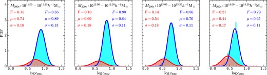
The distribution of the logarithmic halo concentration in four mass bins for relaxed (blue) and unrelaxed (red) haloes, where the criterion to separate these two populations is shown in equation (11). The distribution of both halo populations are fitted with a Gaussian function as shown in solid lines. The best-fitting parameters are shown on the panel.
Fig. 7 shows the halo mass dependence of these fitting parameters. First of all, the unrelaxed haloes only amounts to about 5 per cent of all haloes with |$M_{\rm 200c}\approx 10^{11}h^{-1}\rm M_\odot$|, and this fraction increases to about 15 per cent for |$10^{14}h^{-1}\rm M_\odot$| haloes. The positive correlation between the unrelaxed halo fraction and halo mass is expected, since the halo merger rate is positively correlated to halo mass (e.g. Fakhouri & Ma 2008). Secondly, the mean logarithmic concentration declines with increasing halo mass for both relaxed and unrelaxed haloes, with a constant gap of about 0.28 dex. Finally, the scatter in the distribution of log c for relaxed and unrelaxed haloes are about 0.12 and 0.19 dex, respectively, with a weak dependence on halo mass.
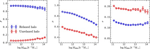
The halo mass dependence of the fitting parameters for relaxed (blue) and unrelaxed (red) haloes, where the left panel shows the halo fraction F, the middle panel the mean log c, and the right panel the standard deviation of log c.
6 OTHER APPLICATIONS OF R1
6.1 Estimating Vmax from R1
The maximum circular velocity, Vmax, is not only a proxy of halo concentration, but also a commonly adopted quantity to connect galaxies with their dark matter haloes (Reddick et al. 2013; Matthee et al. 2017; Zehavi et al. 2019). It is thus important to be able to obtain Vmax efficiently and robustly for a large sample of simulated haloes in order to investigate the galaxy–halo connection using large cosmological simulations. To this end, we derive Vmax from R1 according to equations (4) and (10). Fig. 8 compares the Vmax/Vvir calculated from equation (9) and derived from R1, where one can see they match quite well. We note that there is a small discrepancy for low-mass haloes with high Vmax/Vvir, which has the same origin as the discrepancy for low-mass haloes with high concentrations shown in Fig. 4 (see also Appendix E). Nevertheless, these haloes only account for a small portion of all haloes at the given halo mass bin, as shown in the top panels of Fig. 8. The relative rank is well preserved, as indicated by high Spearman’s rank correlation coefficients (≳0.92).
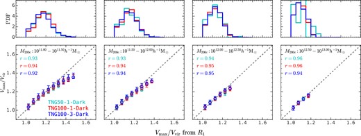
Top panels: the probability distribution of Vmax/Vvir estimated from R1 in three TNG-Dark simulations. Bottom panels: comparison of Vmax/Vvir calculated from equation (9) and from our R1 method in three TNG-Dark simulations. Spearman’s rank correlation coefficients are labelled on the bottom panels.
It should be noted that R1 is defined only for main haloes.3 For a satellite subhalo contained in a host halo, one can trace its main-branch progenitor to the snapshot prior to the infall into its host halo and calculate its R1 to derive Vmax. This is similar to the calculation of Vpeak, which is the peak value of Vmax on the main branch and serves as a better proxy in subhalo abundance matching than Vmax (Reddick et al. 2013). However, it is unclear whether or not environmental effects prior to the infall of haloes can break the relation between Vmax and R1. To test the validity of the R1 method for subhaloes, we compare results between pre-infall haloes at a given redshift, defined as haloes that will become subhaloes in the subsequent snapshot, and the results are presented in Appendix H. There one can see that the Vmax–R1 relation does not depend on whether or not haloes are soon falling into other haloes to become a satellite, indicating that the R1 method can also be used to estimate Vpeak for subhaloes.
6.2 Estimating the Einasto concentration from R1
It has been suggested that the radial density distribution of dark matter haloes in N-body simulations is better fitted with a three-parameter Einasto profile (Navarro et al. 2004; Gao et al. 2008; Wang et al. 2020b), which has the form
where ρ−2, α, and r−2 are free parameters. Gao et al. (2008) found that there is a universal relationship between α and the peak height ν given by
where the peak height ν is defined as the ratio between the critical overdensity δcrit(z) for collapse at redshift z and the linear rms fluctuation at z within spheres containing mass Mvir. We note that the value of ν is determined by redshift and halo mass for a given cosmology. The typical value of α is between 0.15 and 0.3. The concentration parameter for the Einasto profile is defined as
Therefore, at a given redshift of z, the halo mass Mvir and the Einasto concentration ce together determine the halo density profile, with the parameter α determined by equation (13).
Fig. 9 shows the relation between R1 and the Einasto concentration ce for 0.15 ≤ α ≤ 0.3 in circles. And the solid lines are the fitting function,
The bottom panel shows the fractional residual, from which one can see that this fitting function is accurate to |$\lesssim 5~{{\ \rm per\ cent}}$| for ce ≳ 3 and |$\lesssim 10~{{\ \rm per\ cent}}$| for ce ≲ 3.

7 SUMMARY
Estimating the concentration parameter and related quantities of simulated dark matter haloes in large numerical N-body simulations is a critical step to study halo structure and understand its relation to the halo assembly history and to the properties of galaxies that form in them. A reliable and efficient method is needed to estimate these quantities for large cosmological simulations that include haloes with a wide range of particle numbers. To this end, we propose an efficient and robust method to estimate the halo concentration and related quantities using the first moment of the density distribution. Our main results are summarized as follows:
We find that the first moment of the density distribution, defined as |$R_1=\int _0^{r_{\rm vir}}4\pi r^3\rho (r)\mathrm{ d}r^3/M_{\rm vir}/r_{\rm vir}$|, has a simple, monotonic relation with the halo concentration for NFW haloes. A cubic polynomial function can describe this relation to |$\lesssim 3~{{\ \rm per\ cent}}$| accuracy (see Fig. 1).
Testing on ideal NFW haloes, we find that the NFW profile fitting method and the Vmax/Vvir method introduce |$\approx 10~{{\ \rm per\ cent}}$| and |$\approx 30~{{\ \rm per\ cent}}$| systematics for haloes with 100 particles. In contrast, the bias introduced by the R1 method is smaller than 0.5 per cent. The R1 method yields the smallest variance among all the three methods.
Testing on realistic haloes in N-body simulations of different resolutions, we find that the NFW fitting method underestimates the concentration parameter of haloes with ≲300 particles by |$\gtrsim 20~{{\ \rm per\ cent}}$|, due to the poor sampling and the large gravitational softening length. In contrast, such effects only introduce |$\lesssim 8~{{\ \rm per\ cent}}$| systematics in the R1 method (see Figs 3 and 4).
We apply the R1 method to the ELUCID N-body simulation and obtain the mass–concentration relation across four orders of magnitude of halo mass, separately for relaxed and unrelaxed haloes. We find that the distributions of the logarithmic concentration, log c, for both populations can be described by a Gaussian function. We find that the fraction of unrelaxed haloes ranges from |$\approx 5~{{\ \rm per\ cent}}$| to |$\approx 15~{{\ \rm per\ cent}}$| from |$10^{11}$| to |$10^{14}\,h^{-1}\,\rm M_\odot$|. The mean logarithmic concentration declines monotonically with halo mass for both relaxed and unrelaxed haloes, and there is a constant difference of ≈0.28 dex between unrelaxed haloes of lower concentration and relaxed ones with higher concentration. The standard deviations of the logarithmic concentration for relaxed and unrelaxed haloes are ≈0.12 and ≈0.19 dex, respectively, with a weak dependence on halo mass. (see Figs 5, 6, and 7).
The maximum circular velocity, Vmax, of simulated haloes can be derived from R1 efficiently. The Vmax–R1 relation is not affected by whether or not the halo in question is about to be accreted by another halo and to become a subhalo (see Fig. 8 and Appendix H).
We find a fitting function for the relation between R1 and the Einasto concentration ce = rvir/r−2 with 0.15 ≤ α ≤ 0.3, and the fractional deviation is |$\lesssim 5~{{\ \rm per\ cent}}$| for c ≳ 3 and |$\lesssim 10~{{\ \rm per\ cent}}$| for c ≲ 3 (see Fig. 9).
The concentration parameter and related structural quantities of dark matter haloes play an important role in the study of dark matter haloes and the modelling of the galaxy–halo connection. However, because of the uncertainty and tedium in their estimations, many cosmological simulations run in large boxes with relatively low resolutions avoid providing these quantities. The R1 method proposed here can fill the gap, as it provides an accurate proxy for the concentration parameter for both NFW and Einasto haloes. Its estimation is both straightforward and efficient, thus suitable for large cosmological simulations, such as MillenniumTNG (Bose et al. 2023) and FLAMINGO (Schaye et al. 2023). We suggest that this quantity be provided in simulated halo catalogues along with other important halo properties.
ACKNOWLEDGEMENTS
Kai Wang thanks Fangzhou Jiang for his helpful comments and suggestions. The authors acknowledge the Tsinghua Astrophysics High-Performance Computing platform at Tsinghua University for providing computational and data storage resources that have contributed to the research results reported within this paper. This work is supported by the National Science Foundation of China (NSFC) Grant No. 12125301, 12192220, 12192222, and the science research grants from the China Manned Space Project with NO. CMS-CSST-2021-A07. YC is supported by China Postdoctoral Science Foundation Grant No. 2022TQ0329 and NSFC Grant No. 12192224.
The computation in this work is supported by the HPC toolkits hipp (Chen & Wang 2023) and pyhipp,4ipython (Perez & Granger 2007), matplotlib (Hunter 2007), numpy (van der Walt, Colbert & Varoquaux 2011), scipy (Virtanen et al. 2020), and astropy (Astropy Collaboration 2013, 2018, 2022). This research used NASA’s Astrophysics Data System for bibliographic information. The authors thank ELUCID collaboration for making their data products publicly available.5
DATA AVAILABILITY
The data underlying this article will be shared on reasonable request to the corresponding author.
Footnotes
All these models are implemented in the colossus package (Diemer 2018), except Zhao + 09 (http://202.127.29.4/dhzhao/mandc.html) and Correa + 15 (https://www.camilacorrea.com/code/commah/).
We refer to Prof. Martin Weinberg’s lecture note for the detailed derivation in https://courses.umass.edu/astron850-mdw/eddington.pdf.
References
APPENDIX A: GENERATE DARK MATTER HALOES WITH HaloFactory
Here we present an open-source Python package, halofactory,6 which implements the algorithms for generating the position and velocity of particles in mock haloes. These haloes are assumed to be collisionless and spherically symmetric systems in dynamical equilibrium, whose behaviour can be described by the collisionless Boltzmann equation (Binney & Tremaine 2008). halofactory uses Eddington’s inversion method to sample the position and velocity of particles from the exact phase-space distribution function, which is more accurate than approximation methods that rely on the Jeans equations (Binney & Tremaine 2008). In addition, halofactory is rather efficient due to the adoption of various numerical acceleration techniques. Finally, halofactory can serve various purposes, such as providing initial conditions for numerical simulations and serving as input for halo-based galaxy models. Fig. A1 shows the time evolution of the density profile of a halo generated from halofactory with 10 000 particles and an initial concentration of 15. Here one can see that the density profile has nearly no evolution on a time-scale of 10 Gyr, which indicates that the haloes generated from halofactory are already in equilibrium.
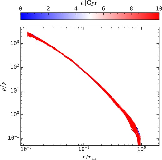
The time evolution of the density profile of a halo with 10 000 particles generated from the halofactory package from 0 to 10 Gyr.
The implementation of halofactory relies on Eddington’s formula. For an equilibrium and spherical system given by the density distribution ρ(r), the particle energy distribution is given by
which is called Eddington’s formula (see chapter 4 in Binney & Tremaine 2008). Here E is the particle energy and V is the potential energy. We also require the maximum energy of particles ET equals to the potential energy at the truncation radius rT, which is a free parameter, so that particles are restrained within rT. In halofactory, the sampling of particle position and velocity are proceeded as follows:
Sampling particle position: We can integrate the radial density profile ρ(r) to get the accumulative mass distribution, which is |$M(\lt r) = \int _0^r 4\pi x^2\rho (x)\mathrm{ d}x$|. Then we generate random numbers |$\mathcal {R}_0$|, which are uniformly distributed between 0 and 1, and solve |$\mathcal {R}_0=M(\lt r)/M(\lt r_{\rm T})$| to get the radial distance. Finally, we randomly sample orientations (θ, ϕ), which are uniformly distributed on a sphere, and the tuples of (r, θ, ϕ) can specify the positions of particles.
- Sampling particle velocity: The sampling of particle velocities relies on Eddington’s formula, which is numerically calculated and tabulated at first.7 We first generate three random numbers |$\mathcal {R}_1$|, |$\mathcal {R}_2$|, and |$\mathcal {R}_3$|, which are uniformly distributed between 0 and 1. Then we can get the radial velocity vr and tangential velocity vt by solving(A2)$$\begin{eqnarray} \mathcal {R}_1 &=& \frac{3}{4}\left[\frac{v_{\rm r}}{v_{\rm max}}-\frac{1}{3} \left(\frac{v_{\rm r}}{v_{\rm max}}\right)^3\right] + \frac{1}{2} \end{eqnarray}$$where |$v_{\rm max}(r) = \sqrt{2(E_T-V(r))}$| is the maximum velocity. Then we evaluate(A3)$$\begin{eqnarray} \mathcal {R}_2 &=& \frac{v_{\rm t}^2}{v_{\rm max}^2-v_{\rm r}^2} , \end{eqnarray}$$and we accept the velocity tuple (vr, vt) if the above assertion is true and otherwise discard it. Finally, we generate an orientation on the plane perpendicular to |$\mathbf {\hat{r}}$| for the tangential velocity component.(A4)$$\begin{eqnarray} \frac{f\left(v_{\rm r}^2/2 + v_{\rm t}^2/2 + V(r)\right)}{f\left(V(r)\right)} \gt \mathcal {R}_3, \end{eqnarray}$$
APPENDIX B: IMPACT OF BINNING ON NFW PROFILE FITTING
Fig. B1 shows the fractional concentration deviation for the NFW profile fitting method on ideal NFW haloes generated from halofactory, and the three rows correspond to the following binning strategies
|$(0.01-1r_{\rm vir}, ~\rm log)$|: 20 equally spaced radial bins on a logarithmic scale from 0.01rvir to rvir, which is used in the main body of the paper;
|$(0.1-1r_{\rm vir}, ~\rm log)$|: 20 equally spaced radial bins on a logarithmic scale from 0.1rvir to rvir (e.g. Bhattacharya et al. 2013);
|$(0-1r_{\rm vir}, ~\rm linear)$|: 20 equally spaced radial bins on a linear scale from 0 to rvir (e.g. Chen et al. 2020);
As one can see, the bias in the first and last binning methods converges to zero as the particle number increases, but the second binning method underestimates the halo concentration, especially for high-concentration haloes. This happens because the second method does not fit the inner density distribution. As the particle number decreases to a few hundred, all three methods produce systematics at the level of |$\approx 10\!-\!20~{{\ \rm per\ cent}}$|, and the sign of the systematics depends both on the binning method and the concentration of the input halo. These results demonstrate that it is not straightforward to find an optimal binning to achieve a reliable estimation of the halo concentration, particularly when individual haloes are only sampled by a small number of particles.
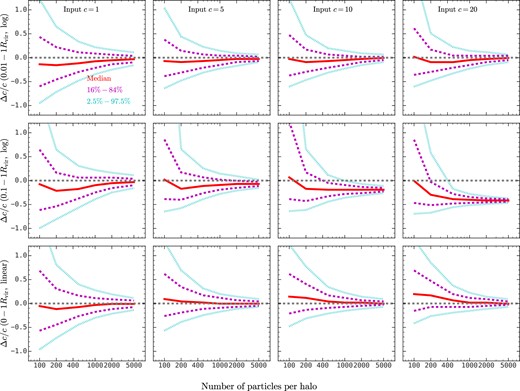
Similar to Fig. 2, except that different rows are the results obtained from the NFW profile fitting method with different binning strategies: binning on a logarithmic scale within 0.01 − 1rvir (top panels), binning on a logarithmic scale within 0.1 − 1rvir (middle panels), and binning on a linear scale within 0 − 1rvir (bottom panels).
APPENDIX C: OTHER METHODS TO ESTIMATE HALO CONCENTRATION
Maximum likelihood: We propose to use the maximum likelihood method to estimate the concentration parameter of NFW haloes. To begin with, the NFW differential mass profile is given by
where m(c) = ln (1 + c) − c/(1 + c), x = r/rvir. Then, for a set of particles, each represented by the normalized radial location xi = ri/rvir, one can express the logarithmic likelihood function as
The concentration parameter can then be estimated by maximizing this likelihood function. We note that the maximum likelihood method is unambiguous and applicable to different halo profiles. However, the summation in the likelihood function needs to be evaluated in each iteration of the optimization, which makes this method computationally expensive, especially for finely sampled haloes.
Peak finding: The NFW differential mass profile (see equation C1) peaks at r = rs, so the concentration parameter c = rvir/rs can be inferred by locating the peak of equation (C1) (e.g. Child et al. 2018). In order to suppress the noise for poorly sampled haloes, we first smooth the differential mass profile with a three-point Hanning filter, which is
Here we calculate the NFW differential mass profile with 20 bins from 0.01rvir to rvir on a logarithmic scale, and the two bins at both ends are dropped after the smoothing step. In this case, the peak is constrained within 0.014rvir and 0.713rvir, so that the minimum and maximum concentrations that can be recovered are 1.4 and 70.3. We note that the result obtained here is subject to the choice of binning.
Cumulative mass: For ideal NFW haloes, the half-mass radius rh, which encloses half of the total halo mass, is given by
where g(x) = ln [(rs + x)/rs] − x/(rs + x). Therefore, the concentration parameter can be inferred through rs by numerically solving this equation (e.g. Lang, Holley-Bockelmann & Sinha 2015).
Fig. C1 shows the performance of these three methods of concentration estimation on ideal NFW haloes. First, the maximum likelihood method performs the best, even outperforming our R1 method (see Fig. 2). This method can be easily generalized to other profiles. However, the optimization of the likelihood is computationally expensive, especially for finely sampled haloes, since the summation of the logarithmic likelihood of all particles needs to be evaluated during each optimization iteration. Secondly, the peak finding method makes no assumption about the specific form of the halo profile. However, this method performs poorly with large systematics and scatter, since it requires the evaluation of the (differential) density profile, which poses challenges to the choice of binning: a large bin size will not sample both ends well, while a small bin size will cause large shot noise. Finally, the cumulative method performs quite well, except for the |$\approx 20~{{\ \rm per\ cent}}$| systematics for poorly sampled high-concentration haloes. Moreover, this method requires numerically solving a non-linear equation, whose complexity is comparable to the conventional NFW profile fitting method.
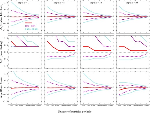
Similar to Fig. 2, except for three other methods to estimate halo concentration: the maximum likelihood method (top panels), the peak finding method (middle panels), and the cumulative mass method (bottom panels).
APPENDIX D: UNCERTAINTIES OF THE R1 METHOD
Here we quantify the statistical uncertainties of our R1 method in estimating halo concentration for ideal NFW haloes. Fig. D1 shows the distribution of the logarithmic deviation of the estimated concentration with our R1 method from the true concentration of ideal NFW haloes. For each input concentration and particle number, we generate 10 000 realizations of NFW haloes and estimate their concentration based on equations (3) and (4). The logarithmic deviation is shown in the grey histogram. We then calculate the standard deviation of the logarithmic deviation as follows:
where Nsamp = 10 000 in this case. Finally, we overplot the probability distribution function of a Gaussian distribution with a mean of 0 and a standard deviation of σ in each panel. Here one can see that this Gaussian distribution matches the histogram very well.
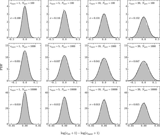
Probability distributions of the deviation of the concentration estimated using the R1 method, cest from the input concentration, cinput for different cinput (different columns) and different numbers of particles (different rows); note the different x-axis ranges. In each panel, the distribution of log (cest + 1) − log (cinput + 1) is shown as a grey histogram, and the standard deviation, σ, calculated with equation (D1) is indicated. A Gaussian distribution of |$\mathcal {N}(\mu =0, \sigma =\sigma)$| is shown in black solid line. This figure shows that the logarithmic deviation of the estimated concentration from the true concentration can be described by a Gaussian distribution.
Fig. D2 shows the relation between σ and the sampling particle number for four different input concentrations. Here one can see that σ is about 0.10–0.15 dex for haloes sampled with only 100 particles. With increasing sampling, the uncertainty of the concentration estimation rapidly decreases, to a value of 0.01 dex when the number of particles reaches 2 × 10⁴. We also find that the dependence of σ on the particle number and the input concentration can be fitted with
where Npart is the particle number. And this function is overplotted in Fig. D2 as solid lines.
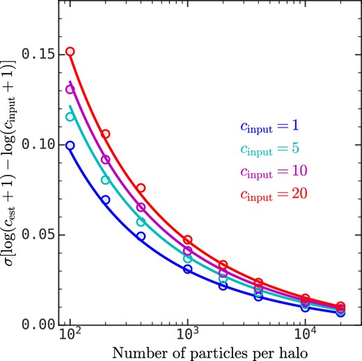
The standard deviation of log (cest + 1) − log (cinput + 1) as a function of particle number per halo for different input concentrations, where cest is estimated with out R1 method. The circles are results obtained with equation (D1) for ideal NFW haloes. The solid lines are the fitting results of equation (D2).
APPENDIX E: DENSITY PROFILE FOR LOW-MASS AND HIGH-CONCENTRATION HALOES
In order to understand the discrepancy in the concentration estimated from the NFW fitting method and our R1 method for low-mass high-concentration haloes in Fig. 4, we select high-concentration haloes with 11 ≤ log (M200c/[h−1M⊙]) < 11.5 from TNG50-1-Dark and plot their density distribution in the right panels of Fig. E1. For comparison, we also plot the density distribution of low-concentration haloes in the same mass range (left panels). Here one can see that the mass distribution of high-concentration haloes deviates from the NFW profile due to stripping in the outskirts of haloes. The density and mass distributions reconstructed from both NFW fitting and R1 methods match the data equally well, despite the |$(18.74-16.32)/18.74\approx 13~{{\ \rm per\ cent}}$| systematics between their results.
![The density distribution of low-concentration (left panels) and high-concentration (right panels) haloes with 11 ≤ log (M200c/[h−1M⊙]) < 11.5 selected from TNG50-1-Dark. The top panels and bottom panels show the density distributions and the mass distributions, respectively. The red solid and blue dashed lines show the NFW profile from the mean concentration of each subsample, where the concentration is estimated with our R1 method and the NFW fitting method, respectively. This figure demonstrates that the discrepancy of concentration estimation from the NFW fitting method and our R1 method for low-mass and high-concentration haloes in Fig. 4 is attributed to the deviation from the NFW distribution due to the stripping of the halo outer regions.](https://oup.silverchair-cdn.com/oup/backfile/Content_public/Journal/mnras/527/4/10.1093_mnras_stad3927/1/m_stad3927fige1.jpeg?Expires=1750340966&Signature=T1ytZEkYs1HgH0biHsfUc2Fu8IhZqBGR1tMev-ctBuz305JR~rgxUTGDfTKk37Nje~uhIOMVfwLYu1VwzmveHVgsBgvskKajoPP5v9zHsM~VJuoDgTJHy2Lj5twEQ01~na2IlUp7oAOJe3P-8UDknZ~imNl~La2cMdPtXPxiAPsd0fAlHoLRYIKthovK4eZ-huUU662tR9lTLziWLUHqxMZRmgogbHGjGn1pL449THxMggWUH8ZgROcp~lOvM8Gpcd8tIRggdQsS6fj5133RvANkGmYeAwzDY-d2L0iA4kTlePd~~-cOWUgG40giYqzHclBZSPRXTgIB8xB~oSmZMQ__&Key-Pair-Id=APKAIE5G5CRDK6RD3PGA)
The density distribution of low-concentration (left panels) and high-concentration (right panels) haloes with 11 ≤ log (M200c/[h−1M⊙]) < 11.5 selected from TNG50-1-Dark. The top panels and bottom panels show the density distributions and the mass distributions, respectively. The red solid and blue dashed lines show the NFW profile from the mean concentration of each subsample, where the concentration is estimated with our R1 method and the NFW fitting method, respectively. This figure demonstrates that the discrepancy of concentration estimation from the NFW fitting method and our R1 method for low-mass and high-concentration haloes in Fig. 4 is attributed to the deviation from the NFW distribution due to the stripping of the halo outer regions.
APPENDIX F: IMPACT OF COSMOLOGY ON THE MASS–CONCENTRATION RELATION
Fig. F1 shows the mass–concentration relation for different cosmological parameters generated from the analytical model in Zhao et al. (2009). Here one can see that the cosmology adopted by TNG yields higher concentrations than that of ELUCID at a given halo mass, as we see in Figs 3 and 5. The bottom panel shows the ratio between these two analytical relations as the black solid line, and the error bars show the ratio between the mass–concentration relations for simulated haloes in TNG100-1-Dark and ELUCID. The two ratios are broadly consistent with each other, indicating that the difference in the mass–concentration relation between TNG100-1-Dark and ELUCID is caused by the different cosmological parameters they adopt.
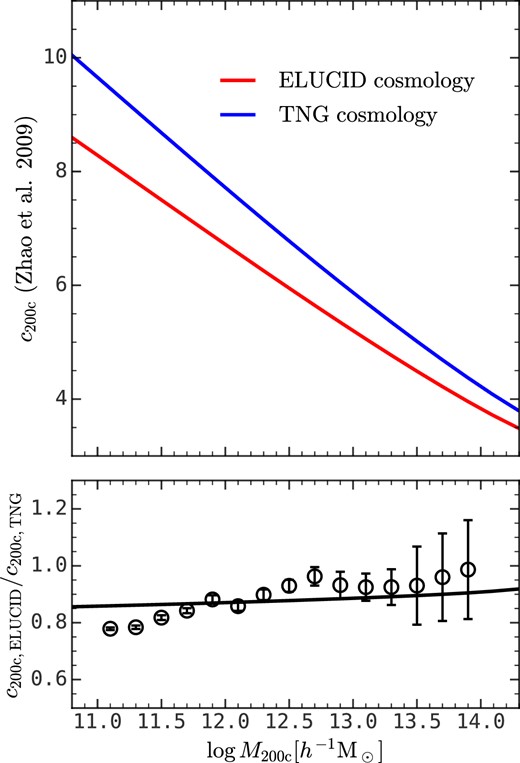
Top panel: The mass–concentration relation generated from the analytical model in Zhao et al. (2009) with the cosmological parameter values used in TNG100-1-Dark and ELUCID (see Section 2). Bottom panel: The ratio between the mass–concentration relations from two different sets of cosmological parameters. The black solid line is the prediction of the model from Zhao et al. (2009), and the black error bars are the result obtained from simulations. The difference of the mass–concentration relation in TNG100-1-Dark and ELUCID can be attributed to the difference in their cosmological parameters.
APPENDIX G: ESTIMATING c200c FROM c500c
Fig. G1 shows the relation between the concentrations obtained from equations (3) and (4) with rvir = r200c and rvir = r500c, which are the radius within which the mean density is 200 and 500 times the critical density, respectively. And the corresponding halo masses are M200c and M500c. The relation between c200c and c500c is fitted with
which has marginal dependence on halo mass. With this relation, we can infer the concentration parameter c200c by integrating equation (3) only to r500c.

APPENDIX H: Vmax ESTIMATION FOR PRE-INFALL HALOES
Fig. H1 compares Vmax/Vvir calculated from equation (9) and estimated from R1 for haloes selected from TNG100-1-Dark at z = 0.7. Here haloes are divided into two subsamples: ‘pre-infall’ haloes are those that will be accreted on to other haloes to become subhaloes in the next snapshot; ‘others’ are haloes excluding ‘pre-infall’ haloes. No additional systematics are seen for pre-infall haloes, indicating that environmental effects on superhalo scales have insignificant effects on the estimation of Vmax/Vvir from R1.
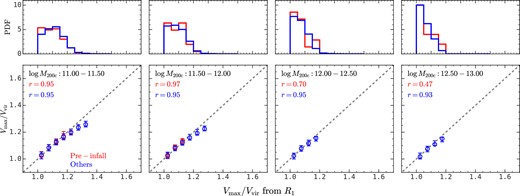
Similar to Fig. 8, except that these haloes are selected from TNG100-1-Dark at z = 0.7. The red error bars are for haloes that will be accreted by other haloes and become a satellite subhalo at the next snapshot, and blue error bars are for the remaining haloes. The environmental effects before accretion do not affect the estimation of Vmax/Vvir from R1.
