


ABSTRACT
We investigate non-linear structure formation in the context of the fuzzy dark matter (FDM) model and compare it to the cold dark matter (CDM) model from a weak lensing perspective. Employing Eulerian perturbation theory (PT) up to fourth order, we calculate the tree-level matter trispectra and the one-loop matter spectra and bispectra from consistently chosen initial conditions. Furthermore, we conduct N-body simulations with CDM and FDM initial conditions to predict the non-linear matter power spectra. Subsequently, we derive the respective lensing spectra, bispectra, and trispectra for CDM and FDM within the framework of a Euclid-like weak lensing survey. In our analysis, we compute attainable cumulative signal-to-noise ratios and estimate χ2-functionals, aimed at distinguishing FDM from CDM at particle masses of m = 10−21 eV, m = 10−22 eV, and m = 10−23 eV. Our results indicate that PT predictions are insufficient for distinguishing between the CDM and FDM models within the context of our simulated weak lensing survey for the considered particle masses. Assuming that N-body simulations overestimate late-time small-scale power in the FDM model, future weak lensing surveys may provide the means to discriminate between FDM and CDM up to a mass of m = 10−23 eV. However, for stronger constraints on the FDM mass, observations of the local high-z universe may be more suitable.
1 INTRODUCTION
The fuzzy dark matter (FDM) model, initially proposed by Hu, Barkana & Gruzinov (2000), describes dark matter as a bosonic, scalar field composed of very light particles with typical masses m ∼ 10−22 eV, exhibiting negligible self-interactions and possessing a macroscopic de Broglie wavelength. In the non-relativistic regime, the dynamics of FDM are governed by the Schrödinger–Poisson system (SPS) of equations. Due to its small mass, the FDM boson has an astrophysically relevant de Broglie wavelength on the order of a few kiloparsecs. FDM represents a small-scale modification of cold dark matter (CDM), governed by the particle mass. Its wave-like behaviour suppresses structure formation on small scales, while CDM-like behaviour is recovered on larger scales. Consequently, the FDM model holds the potential to address the small-scale crisis of CDM.
The FDM bosons are also called axions or axion-like particles. Axion-like particles with exponentially suppressed masses are naturally generated in supersymmetric theories and theories with extra-dimensions including string theory (Marsh 2016). A currently popular FDM model is one where all dark matter is composed of axions with m ≈ 10−22 eV (Hu, Barkana & Gruzinov 2000; Marsh 2016). This mass has also been suggested by Schive, Chiueh & Broadhurst (2014) who fitted the ground-state density of a halo obtained in a numerical simulation of FDM to the mass distribution of the Fornax dwarf spheroidal galaxy. However, the allowed range of FDM masses that could solve the small-scale crisis of CDM is increasingly narrowed down by various observations:
Armengaud et al. (2017); Iršič et al. (2017); Kobayashi et al. (2017) constrain the FDM mass using measurements of the Ly α forest flux spectrum from the XQ-100, HIRES/MIKE, SDSS/BOSS, and XSHOOTER data sets and derive bounds between m > 7.1 × 10⁻²² eV and m > 2.3 × 10⁻²¹ eV. The biggest uncertainties in their approach stem from the modelling of the observed fluctuations in the neutral hydrogen and the use of hydrodynamical CDM simulations using FDM initial conditions (ICs), thereby neglecting FDM dynamics at late times. Nori et al. (2018) improve on these results by including the effect of the quantum pressure term in their N-body simulations and derive the bound m > 2.1 × 10⁻²¹ eV. The fact that the different groups’ results are consistent indicates that the effect of late-time FDM dynamics on the Ly α flux power spectrum may be negligible. At the same time, Zhang et al. (2018) carefully examine the Ly α forest constraints on FDM and conclude that full FDM simulations are required for reliable constraints based on the Ly α forest. They also point out that the uncertainties of hydrodynamics simulations and the thermal properties of the intergalactic medium (IGM) may have been underestimated in previous studies. Rogers & Peiris (2021) improve on the modelling of the IGM by using a new, robust N-body-based modelling pipeline marginalizing over an IGM model which allows for a wide range of heating and ionization histories. They find a stronger bound of 2 × 10⁻²⁰ eV (95 per cent C.L.). Note that modifications of FDM such as the extreme-axion FDM model that features single-mass FDM dynamics with a modified linear matter power spectrum may provide another avenue to relieve the FDM constraints posed by the Ly α forest observations (Leong et al. 2019).
Order unity density fluctuations as a result of wave interference in haloes are a robust and well-understood prediction of the FDM model. They are expected to dynamically heat stellar orbits in ultra-faint dwarf galaxies (UFDs). Marsh & Niemeyer (2019) compute the gravitational heating of a star cluster in the UFD Eridanus II and find that the mass range 0.8 × 10⁻²¹ eV <m < 1.0 × 10⁻¹⁹ eV is disfavoured. Moreover, they find that the formation of Eridanus II as a subhalo demands m ≳ 0.8 × 10⁻²¹ eV. Schive, Chiueh & Broadhurst (2020) use FDM simulations to demonstrate that the random walk which the central soliton in the FDM halo undergoes, represents an even bigger challenge for the survival of the central star cluster in Eridanus II. As a possible solution, they argue that the star cluster could survive the soliton random walk if the FDM subhalo had been tidally stripped by the influence of the Milky Way’s gravitational potential.
Dalal & Kravtsov (2022) derive the bound m > 3 × 10⁻¹⁹ eV by showing that the dynamic stellar heating predicted by FDM is not consistent with the observed stellar velocity dispersion in the UFDs Segue 1 and Segue 2. Amorisco & Loeb (2018) study the dynamical heating of thin stellar streams through the density granulation in FDM haloes and find the limit m > 1.5 × 10⁻²² eV. In a similar spirit, Church, Mocz & Ostriker (2019) study the dynamical heating of galactic discs in CDM and FDM and find the lower bound m > 0.6 × 10⁻²² eV.
The inner density profile of dwarf galaxies provides another way of testing FDM predictions. Calabrese & Spergel (2016) and Chen, Schive & Chiueh (2017) compare the flat, inner density profile of Milky Way dwarf satellites to the inner solitonic profile of FDM haloes and find m ≈ 1 × 10⁻²² – 6 × 10⁻²² eV. Safarzadeh & Spergel (2020) point out that while the FDM prediction for m ≳ 10−21 eV matches the profiles of the known UFD Milky Way satellites, the density profiles of the dwarf spheroidals Fornax and Sculptor, originally considered by Schive, Chiueh & Broadhurst (2014), disagree with the FDM predictions. In turn, a mass around 10−22 eV seems to suggest that the mass of the UFDs is too large. In other words, no single-FDM mass seems to be able to account for the density profiles of all known dwarf galaxies.
Another constraint on the FDM mass can be derived from the circular velocity in disc galaxies. Assuming the soliton–host halo mass relation empirically found by Schive, Chiueh & Broadhurst (2014), Bar et al. (2018); Bar, Blum & Sun (2022) argue that the peak circular velocity characterizing the host halo on large scales should repeat itself in the central region and rule out FDM masses in the range m = 10−24 − 10−20 eV.
Using the subhalo mass function inferred from the observed luminosity function of Milky Way satellites, Nadler et al. (2021) constrain the warm dark matter, self-interacting dark matter, and FDM models alike and obtain the bound m > 2.9 × 10⁻²¹ eV (|$95~{{\ \rm per\ cent}}$| C.L.) on the FDM mass. Uncertainty comes from the prediction of the halo mass function from the linear power spectrum. A further mass constraint based on the early formation of haloes is given by Lidz & Hui (2018) who use the hyperfine 21 cm transition of hydrogen at redshifts between z = 15 and z = 20 to constrain the FDM mass to be m > 5 × 10⁻²¹ eV.
Future surveys of the 21-cm power spectrum such as HERA are expected to be sensitive to FDM masses up to 10−18 eV if all of the cosmological dark matter is fuzzy. In addition, they are sensitive to small FDM fractions around 1 per cent in the mass range 10−25 eV ≲ m ≲ 10−23 eV (Hotinli, Marsh & Kamionkowski 2022).
Superradiance rules out FDM masses in the mass range from m = 10−21 − 10−17 eV (Ünal, Pacucci & Loeb 2021). Davies & Mocz (2020) study solitons with supermassive black holes at their centre and exclude 10−22.12 eV ≲ m ≲ 10−22.06 eV. González-Morales et al. (2017) find the upper bound of m < 0.4 × 10⁻²² eV (|$97.5~{{\ \rm per\ cent}}$| C.L.) by fitting the luminosity-averaged velocity dispersion of dwarf spheroidal galaxies. Sarkar, Pandey & Sethi (2021) constrain the FDM mass to be m > 0.2 × 10⁻²² eV (1σ) by studying the Ly α effective opacity. Maleki, Baghram & Rahvar (2020) find m > 0.7 × 10⁻²² eV by studying X-ray emissions during solitons mergers.
Gravitational lensing provides yet another complementary probe in addition to the aforementioned constraints. Powell et al. (2023) study the granular structure in the main dark matter halo of a single-gravitational lens system and derive the bound m > 4.4 × 10⁻²¹ eV. For lower masses, Hložek, Marsh & Grin (2018) identify the possible mass range for FDM via CMB lensing based on the full Planck data set and find no evidence for an FDM component in the mass range 10−33eV ≤ m ≤ 10−24 eV. More recently, Rogers et al. (2023) combine the Planck CMB data and galaxy power spectrum and bispectrum data from the BOSS survey to conclude that FDM with m ≤ 10−26 eV makes up less than 10 per cent and FDM with 10−30 eV ≤m ≤ 10−28 eV makes up less than 1 per cent of dark matter today.
To sum up, essentially the entire mass range from m = 10−26 eV to m = 10−16 eV is under tension with various observations. The m ≈ 10−22 model is particularly constrained by the Ly α forest, galactic rotation curves, dynamical heating arguments, the subhalo mass function, and strong lensing.
In this work, we estimate whether future weak lensing surveys have the constraining power to further complement some of the existing constraints on the FDM mass. Weak lensing surveys such as Euclid measure the lensing shear spectrum and allow inferring the shape and amplitude of the matter spectrum Pδ, thereby giving constraints on cosmological parameters such as the axion mass. Gravitational lensing probes the matter distribution without any biasing assumption. This is important because the preferred value of the galaxy bias b and therefore the normalization of the galaxy spectrum are different for FDM than for ΛCDM. As a consequence, the constraining power of galaxy surveys on the FDM mass is lower than that of weak lensing.
In the existing literature on weak lensing studies of FDM, Marsh et al. (2012) analyse whether adding a small fraction of axions of mass in the range m = 10−29 eV would be detectable via the lensing convergence spectrum. For modelling non-linearities, they neglect the quantum pressure and employ the CDM halofit model implemented in the camb code (Lewis, Challinor & Lasenby 2000). Dentler et al. (2022) combine CMB Planck data with shear correlation data from the Dark Energy Survey Year 1 and find m > 10−23 eV (95 per cent C.L.). They model the non-linear FDM spectra using the adapted halo model hmcode. Lensing can also serve as a tool to investigate axion-related isocurvature fluctuations (Feix et al. 2019, 2020), with a sensitivity to axion masses at the scale 10−19 eV. In contrast, we estimate the spectra, bispectra, and trispectra using fluid perturbation theory (PT). To this end, we recast the SPS into a hydrodynamical form using the so-called Madelung transform. The Madelung equations are Euler–Poisson equations with an additional scale-dependent modification, the so-called quantum pressure term. On large scales, this term vanishes and one recovers the ideal fluid equations for CDM. One of the appeals of the Madelung transform lies in being able to apply standard cosmological PT to the SPS. Its range of validity is higher than that of wave PT and one can easily contrast it with PT in CDM (Woo & Chiueh 2009; Li, Hui & Bryan 2019). Whether the inherently higher degree of small-scale anisotropy in FDM (Dome et al. 2022) can differentiate between dark matter models remains to be investigated.
Building on and extending the work of Li, Hui & Bryan (2019) who compute the one-loop matter spectrum for FDM, we use time-dependent non-linear Eulerian PT up to fourth order to compute the tree- and loop-level bispectra as well as the tree-level trispectra. To estimate the range of validity of our results, we compare the PT predictions with a set of N-body simulations with CDM and FDM ICs. We go on to derive the corresponding lensing spectra for a Euclid-like lensing survey. We estimate the attainable signal-to-noise ratios as well as the χ2-functional for distinguishing axions of the masses m = 10−21 eV, m = 10−22 eV and m = 10−23 eV from standard CDM. These masses are interesting because they cover the range of masses that might solve the small-scale crisis of CDM.
The outline of this paper is as follows: Section 2 introduces the SPS, presents linear and non-linear Eulerian PT for FDM and computes the matter spectra, bispectra, and trispectra. Section 3 introduces the basics of weak lensing surveys, computes the respective lensing spectra and estimates the attainable weak lensing signal-to-noise ratios and χ2-functionals. Section 4 summarizes and discusses the results. Appendices A through C list the technical and numerical details of the FDM PT. Appendix D lists the details of the N-body simulations.
2 NON-LINEAR STRUCTURE FORMATION WITH FDM
Consider a (pseudo-)scalar field φ minimally coupled with gravity:
where we follow the convention in Hui et al. (2017). m is the axion mass, which naturally appears in the Compton scale λ = ℏ/(mc). This action is invariant under parity- and time-inversion because it is quadratic in φ. For QCD axions, this action is applicable after symmetry breaking and after non-perturbative effects have been switched on. Furthermore, we neglect possible non-gravitational self-interactions of the axion in the form of an axion potential V(φ). In our discussion, it will not be important whether the FDM particle is an axion-like particle or not. We only assume that the particle is bosonic, non-relativistic, has negligible self-interaction and makes up the entirety of dark matter. We can study solutions of the relativistic axion equation of motion for a perturbed Friedmann–Lemaître–Robertson–Walker (FLRW) metric including a cosmological constant Λ, all in Newtonian gauge. This is appropriate for studying structure formation because the virial velocity in a typical galaxy |$\upsilon _\mathrm{vir} \sim 100 \frac{km}{s} \ll c$| and galaxies are much smaller than the Hubble horizon. At the same time, we consider scales larger than the axion Compton wavelength which would correspond to relativistic scales in the Klein–Gordon equation. Except in the vicinity of black holes, the Newtonian potential Φ obeys |Φ|/c2 ≪ 1. To study the clustering of axions on non-linear scales, we further apply the Wentzel–Kramer–Brillouin approximation of the form
where ψ is a complex scalar field. In addition, we assume Φ ∼ ϵ2, k/m ∼ ϵ and H/m ∼ ϵ, keeping terms up to order |$\mathcal {O}(\epsilon ^2)$|, as well as the non-relativistic approximation |$|\dot{\psi }| \ll \frac{mc^2}{\hbar }|\psi |$|. The assumption |$\partial _t \ll m$| is non-relativistic because we have |$\partial _t \sim \Delta /m \sim k^2/m$| and therefore k2/m ≪ m. With these simplifications, we obtain the comoving Schrödinger–Poisson system of equations
where ρb(t) is the background density and |ψ|2 measures the density in a proper volume. We supplement the Schrödinger–Poisson equations with the normalization condition
which fixes the density ρ = |ψ|2 for N axions of mass m. In equation (3), positions of particles are described using comoving coordinates |$\boldsymbol {x}$|.
2.1 Quantum pressure and Jeans scale
The Madelung transform (Madelung 1927) follows by substituting
for real fields ρ(x, t) and S(x, t) into equation (3). Defining the velocity field
we obtain the Madelung equations
The Madelung equations describe the Schrödinger equation via a system of fluid equations for frictionless, compressible flow in an external gravitational potential Φ. The flow gets modified by the quantum pressure QP with
The quantum pressure accounts for the underlying wave dynamics in FDM. For a narrowly located source, the quantum pressure is large and reflects the Heisenberg uncertainty principle in quantum mechanics.1 On large scales, the Madelung equations reduce to the Euler equations of a pressureless fluid and we recover the dynamics of CDM. The quantum pressure QP is equivalent to an anisotropic pressure stress Pij, where
We can describe the linearized evolution of the density contrast by assuming δ ≪ 1 and |$\left|\boldsymbol {\upsilon }\right| \ll 1$| for the fluctuation fields and neglecting higher-order perturbations of the form |$\mathcal {O}(\delta ^2, \upsilon \delta , \upsilon ^2)$| to obtain
For each mode k, equation (11) describes a harmonic oscillator with time-dependent dampening H(t) and frequency ω(k, t) as
Unlike in the CDM case, linear growth in FDM is scale-dependent because of the quantum pressure term. The condition ω = 0 defines the comoving quantum Jeans scale kJ (see Khlopov, Malomed & Zeldovich 1985):
The Jeans scale describes a force balance between gravity and quantum pressure. For k < kJ, ω(k, t) becomes imaginary and we recover a growing and a decaying mode. Perturbations on these scales are unstable and will gravitationally collapse. For k > kJ, the frequency ω(k, t) becomes real. Perturbations on small scales therefore undergo oscillations and are stabilized against gravitational collapse. The comoving Jeans wavelength decreases with time as |$\lambda _J \sim a^{-\frac{1}{4}}$| which is why more small-scale features can develop as the universe expands. We can find an analytical solution of the linear FDM growth equation (11) in the Einstein–de-Sitter (EdS) case for Ωm = 1. To this end, we substitute the ansatz |$\delta (\boldsymbol {x}, a) = \delta (\boldsymbol {x}, a=a_0) D(a, a_0)$| into equation (11) and rewrite the resulting ODE for the growth factor D in terms of the scale factor a
Simplifying with Ωm, 0 = 1 yields
Chavanis (2012) and Suárez & Chavanis (2015) study solutions of equation (15) in terms of Bessel functions in the context of Bose–Einstein condensate dark matter with self-interaction and the weak-field limit of the Klein–Gordon–Einstein equation. They find
where J∓5/2 are cylindrical Bessel functions of fractional order
Li, Hui & Bryan (2019) give a solution of equation (15) with D±(k, a0, a0) = 1 in terms of the solutions equation (16) as
We immediately notice that equation (19) can exhibit unphysical divergences at the roots of the Bessel function. Laguë et al. (2020) argue that this is simply a matter of choice of normalization, but this is not quite true. Equation (19) is not a solution of the linear growth equation (15) if it diverges in the domain of interest. We are not aware of a general analytical solution to equation (15), even in the EdS case. Laguë et al. (2020) suggest two ways to remedy this issue: One way is to approximate the denominator of equation (19) by a fifth-order Taylor expansion of the Bessel function which removes divergences from equation (19) and gives fewer oscillations. In contrast, a different number of terms in the Taylor expansion leads to fast oscillations and/or divergences. An alternative that Laguë et al. (2020) adopt is to use a model for the mean growth of the FDM growth function. They describe the growing mode D+ in terms of a smoothed Heaviside step function where free parameters are determined via a fit to the axionCAMB transfer function (Hlozek et al. 2014). For large scales, this approach exactly recovers the CDM growth function but has the disadvantage that oscillations are entirely neglected. Moreover, the smoothed Heaviside step function falls off exponentially for large k which is not a correct description of the asymptotic behaviour of D+. We therefore opt for integrating equation (15) numerically. As ICs, we choose
where |$D_{\mathrm{CDM}}^{\prime }(a_0)$| is obtained via numerical integration of the linear growth equation (14) for ℏ = 0 corresponding to CDM. This approach has several advantages: We ensure D(k, a0, a0) = 1 via the ICs and obtain the correct CDM evolution in a general cosmology in the limit k → 0. Further and most importantly, the growth factor obtained in this way is a solution to the linear growth equation (15). It does not exhibit unphysical divergences as shown in Fig. 1. We see that the numerical solution of the growth equation also exhibits the correct asymptotic behaviour |$\lim _{k\rightarrow \infty } \frac{D_{\mathrm{FDM}}(k, a)}{D_{\mathrm{CDM}}(a)} = 0.$|
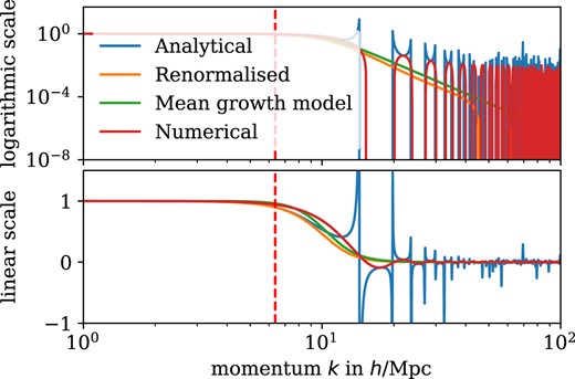
Asymptotic behaviour of growing modes represented via the quotient of FDM and CDM growth factors D+, FDM(k, a)/D+, CDM(a) in a EdS universe filled with FDM with a mass of m = 10−23 eV. The graphs show the analytical, divergent expression (19), the renormalized expression using the fifth-order Taylor expansion, the numerical solution obtained by integrating the linear growth equation with ICs given by equation (20) as well as a mean growth model |$D(k, a) \approx \Bigl (1 + \alpha \left(\frac{k}{k_J}\right)^{\beta }\Bigl) D_{\mathrm{CDM}}(a)$| with the fit parameters α = 0.17, β = 6.50 obtained via fitting to the analytical solution.
In addition, the numerical solution captures the oscillatory behaviour of the analytical solution for high k. At the same time, there are also several disadvantages of numerically integrating the linear growth equation in FDM. First, we do not capture the growing mode in the oscillating regime. This is because we do not know the correct ICs for the growing mode. Therefore, the numerical solution in the oscillating regime will in general be a linear combination of the two modes D+ and D−. However, since the physically correct ICs for the linear fluctuation fields are unknown, this does not add any uncertainty to the linear growth model in terms of ICs. In any case, we recover the correct modes for a > aosc. This is because any component proportional to D− in the ICs quickly decays for a > aosc. Fig. 2 shows the growing solutions obtained for a fiducial cosmology with Ωm, 0 = 0.3159 and a dark energy equation of state w = −0.9 used in the rest of this work.
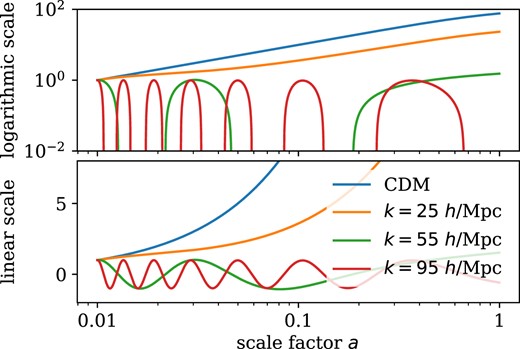
Growing modes D+(a) in CDM and D+(k, a) in FDM in fiducial cosmology obtained by numerical integration of equation (15) for ℏ = 0 (CDM) and a mass of m = 10−22 eV at three different scales k (FDM). Growth factors are normalized to D+(a0) = 1 at a0 = 0.01.
To sum up, the key difference between CDM and FDM in linear PT is the existence of a unique length-scale in FDM. Whereas all scales are gravitationally unstable in CDM, the perturbations below the quantum Jeans scale are stabilized in FDM. Nonetheless, non-linear PT may alter these conclusions since the quantum Jeans scale is a concept only valid within linear PT. This can be seen by taking the first few terms of the Taylor expansion of the quantum pressure equation (9): |$\frac{2m^2}{\hbar ^2} \Delta Q_P = - \Delta \frac{\Delta \sqrt{\rho }}{\sqrt{\rho }} = \Delta \left(- \Delta \delta + \frac{1}{4} \Delta \delta ^2 + \frac{1}{2} \delta \Delta \delta + \mathcal {O}(\delta ^2) \right)$|. The linear contribution −Δ2δ counteracts gravity. However, the quadratic term acts in the same direction as gravity and could therefore potentially enhance gravitational collapse (Li, Hui & Bryan 2019). This is related to the fact that the interference of waves can lead to structures that are smaller than their wavelength. To estimate the effect of non-linearities on cosmological structure formation, we develop a non-linear PT for CDM and FDM in the further section.
2.2 Tree- and loop-level PT
The goal of cosmological PT is to describe the departure of matter evolution from the homogeneous Hubble expansion perturbatively. In Eulerian PT, one describes the non-linear gravitational dynamics in terms of solutions δ(1) and |$\boldsymbol {\upsilon }^{(1)}$| of the linearized fluid equations in a fixed laboratory frame:
where |$\theta = \nabla \cdot \boldsymbol {\upsilon }$| and the nth-order fluctuation fields δ(n) and θ(n) are proportional to the nth power of the linear fluctuation fields:
In addition, the linearized continuity equation implies |$\partial _a \delta ^{(1)} = \theta ^{(1)}$|. Therefore, both the velocity and the density field are fully determined by the linear density fluctuations. The coupling of linear modes in the non-linear theory is described by the non-linear coupling kernels Fn and Gn:
where Fn and Gn are homogeneous functions of the wave vectors |$\boldsymbol {q}_1, \ldots , \boldsymbol {q}_n$| with degree zero and |$\boldsymbol {q}_{1, \ldots , n} \equiv \boldsymbol {q}_1 + \ldots + \boldsymbol {q}_n$|. A series of papers (Fry 1984; Goroff et al. 1986; Jain & Bertschinger 1994) developed a method for deriving the time-independent CDM mode coupling kernels in terms of algebraic recursion relations. They rely on the Euler–Poisson system being homogeneous in the scale factor a in the EdS case. Including the quantum pressure breaks this homogeneity and just like for a general cosmology in CDM, the solutions at each order become non-separable functions of time and scale.
A method to nonetheless obtain the PT kernels is described in the series of papers (Scoccimarro 1998, 2006) that developed time-dependent Eulerian PT with the aid of Feynman diagrams. Effectively, Li, Hui & Bryan (2019) use this method to compute the kernels F2 and F3 in FDM. The non-linear terms in the Madelung equations are treated as inhomogeneity g(η) while solving the linear growth equation. This leads to an integral equation that can be represented as a Dyson series. The Dyson series allows for a diagrammatic representation and can be recursively solved up to a given order in PT. In Appendix A, we retrace the steps taken by Li, Hui & Bryan (2019) and extend them to higher order in PT for the consistent tree- and loop-level computation of bi- and trispectra in FDM, which necessitates the kernels F2, F3, and F4. Recent developments in PT recast this straightforward perturbative approach into more powerful formalisms (Pietroni 2008; Bartelmann et al. 2016; Kozlikin et al. 2021) including FDM (Littek 2018).
2.3 Spectra, bispectra, and trispectra at tree and loop level
We derive explicit expressions for the kernels F2, F3, and F4 in the FDM and CDM case in Appendix A. These kernels Fn can then be used to perturbatively expand n-point-matter correlation functions |$P_n(\boldsymbol {k}_1, \boldsymbol {k}_2, \ldots , \boldsymbol {k}_n)$|. The latter are defined as the Fourier transform of the connected correlation functions:
In the following, we are interested in the equal-time matter spectrum P ≡ P2, bispectrum B ≡ P3, and trispectrum T ≡ P4. We express the n-point correlations of non-Gaussian perturbations as integrals over higher-order correlations of Gaussian perturbations. We then apply Wick’s theorem to express higher-order correlations of Gaussian perturbations as two-point correlations of Gaussian perturbations. The latter are completely specified by the ICs. Expanding the two-point correlation as a perturbation series |$P(k, a) = P^{(0)}(k, a) + P^{(1)}(k, a) + \ldots$|, we find that the time evolution of the linear spectrum P(0) can be expressed as linear scaling of the initial spectrum:
In the following, we omit the explicit time dependencies. The first higher-order contribution P(1) to the spectrum comes at loop level.2 The two loop-level contributions to the one-loop spectrum P(1) are given by
with
The bispectrum at tree level corresponding to second-order PT is given by
The one-loop contribution to the bispectrum consists of four distinct diagrams involving up to fourth-order PT kernels:
whose explicit expressions are given by
In the following, we also examine the reduced bispectrum
It is independent of time and normalization. For scale-free ICs P(0), that is, P(0)∝kn with the spectral index n, Q(0) is also independent of overall scale and for equilateral configurations it is also independent of the spectral index. Finally, the diagrams for the trispectrum involve vertices connecting two and three lines and therefore correspond to second-order and third-order PT. One can decompose the tree-level trispectrum into the contributions
where
We now present the different spectra computed with time-dependent PT in CDM and FDM for a dark energy cosmology with w = −0.9 and Ωm, 0 = 0.3159 at z = 0. For computing the non-linear PT kernels Fn, we use the EdS growth factors in both CDM and FDM.3 The initial spectra are computed using the camb and axionCAMB codes for CDM and FDM, respectively (Lewis, Challinor & Lasenby 2000; Hlozek et al. 2014). Importantly, the non-linear CDM matter power spectra obtained via N-body simulations and PT are only expected to agree to percent level up to k ∼ 0.1 h Mpc−1 at z = 0 (Carrasco et al. 2014). Therefore, we also run a total of 8 N-body simulations in two boxes with sizes L = 256 Mpc h−1 and L = 30 Mpc h−1 featuring N = 5123 particles using the gadget-2 code (Springel 2005). The L = 256 Mpc h−1 box provides a cross-check of the large-scale loop-level PT matter power spectra. The L = 30 Mpc h−1 simulations are used to obtain a rough estimate of the fully non-linear matter power spectra on small scales. Since we probe the matter power spectrum at late times and on scales smaller than the Jeans scale, we expect the effect of the quantum pressure to be important. Armengaud et al. (2017) note that especially for masses smaller than m ∼ 10−22 eV, the quantum pressure affects a significant portion of the dark matter particles on scales k ≳ 1 h Mpc−1. Therefore, the N-body power spectra for the m = 10−22 eV and m = 10−23 eV cases are expected to exhibit large errors on small scales that could only be eliminated with large-scale FDM simulations including wave dynamics which are arguably beyond the reach of current supercomputers. To the authors’ knowledge, May & Springel (2021, 2022) perform the largest high resolution wave-based simulations of the FDM model to date. They employ a mass of m = 7 × 10⁻²³ eV in a L = 10 Mpc h−1 box and compare CDM and FDM simulations both with CDM and FDM IC at different times up to z = 3. They observe that the effect of the quantum pressure generally leads to further suppression of small-scale power, except for a feature at k ∼ 1000 h Mpc−1 where the FDM spectrum slightly exceeds the CDM spectrum – likely as a result of wave interference. Nori et al. (2018) also compare N-body simulations with and without quantum pressure up to z = 0 and find that the quantum pressure reduces small-scale power. Therefore, we believe that the N-body simulations serve as an important cross-validation. Technical details can be found in Appendix D.
Fig. 3 shows the CDM and FDM spectra at tree level and with loop-level corrections as well as the spectra from several N-body simulations with FDM and CDM IC at z = 0. At tree level, power is strongly suppressed below the Jeans scale in the FDM model. Non-linear corrections at loop level transfer power to small scales, but suppression is still dominant. As previously noted by Nori & Baldi (2018) and Nori et al. (2018), the initial suppression of power on small scales in the N-body simulations is almost completely overcome by late-time non-linear CDM dynamics. Note that the low-k modes in the N-body simulations suffer from large variations due to a low sample number. Moreover, there is a mismatch between the high-k modes of the L = 256 Mpc h−1 and the low-k modes of the L = 30 Mpc h−1 simulations at k = 6 h Mpc−1 indicated by the vertical grey line. This is because the L = 30 Mpc h−1 box is too small for the large-scale modes to evolve correctly. Fig. 4 shows the respective spectra at z = 6.1 for reference. The loop-level PT and the N-body results agree up to k = 1 h Mpc−1, but still start to differ on smaller scales. The different N-body power spectra demonstrate that late-time CDM dynamics have not yet overcome the initial suppression of power on small scales at z ∼ 6.
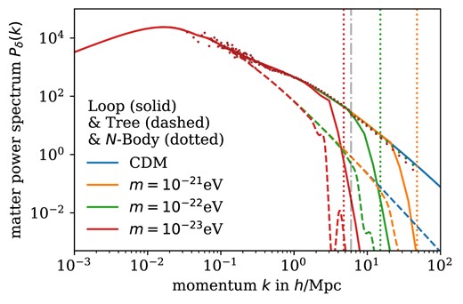
Dark matter spectra Pδ(k) at tree and loop level as well as from N-body simulation at z = 0. The N-body results overlap. The dashed, grey line indicates the transition between the simulation boxes of different sizes. The dotted, vertical lines denote the respective Jeans scales from equation (13) at z = 99.
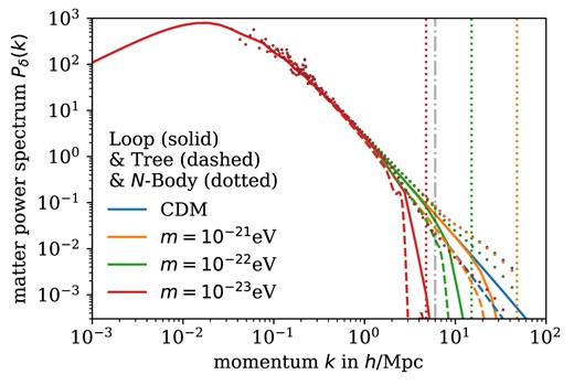
Dark matter spectra Pδ(k) at tree and loop level as well as from N-body simulation at z = 6.1. The dashed, grey line indicates the transition between the simulation boxe of different size. The dotted, vertical lines denote the respective Jeans scales from equation (13) at z = 99.
Figs 5 and 6 show the equilateral matter bispectra and equilateral square matter trispectra. Figs 11 and 12 show the respective convergence spectra. As in the case of the spectrum, loop-level corrections for the bispectrum have the effect of adding power on small scales in both CDM and FDM. At both tree and loop level, however, suppression below the Jeans scale is still the dominant effect in FDM.
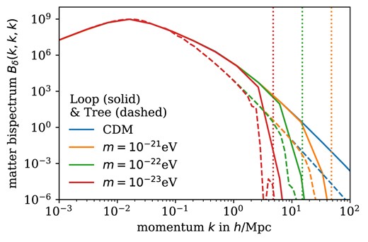
Equilateral dark matter bispectra Bδ(k, k, k) at tree and loop level at z = 0. The dotted, vertical lines denote the respective Jeans scales from equation (13) at z = 99.
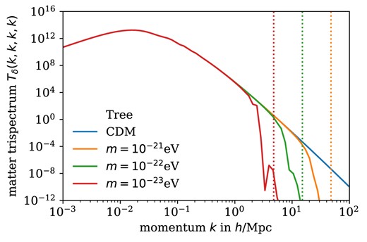
Equilateral square matter trispectra Tδ(k, k, k, k) at tree level at z = 0. Dashed lines indicate respective Jeans scales from equation (13) at z = 99.
The loop-level corrections given by equation (27) were computed in a form free of infrared divergences using the cuba library (Hahn 2005). Details of the numerical integration can be found in Appendix C. Fig. 7 shows the angular dependence of the reduced matter bispectrum Q(0) at tree level. The fact that Q(0) is enhanced for θ = 0, π reflects the fact that large-scale flows generated by gravitational instability are mostly parallel to density gradients. As discussed in subsection 2.1, the kernel |$F_2^{(s)}$| includes the first higher-order correction from the quantum pressure term. Therefore, it does not only counteract gravitational collapse but can also enhance it as is exemplified by the graphs for m = 10−21 eV and m = 10−22 eV at scales k around or below the Jeans scale for the respective masses.
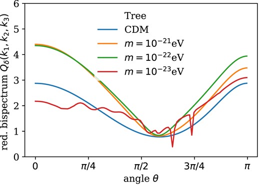
Angular dependence of reduced bispectra at tree level with |$\theta = \sphericalangle (\boldsymbol {k}_1, \boldsymbol {-k_2})$| with k1 = 10 h Mpc−1 and k2 = 0.1 h Mpc−1 at z = 0. The graph for m = 10−23 eV is in the oscillating regime and its shape depends on how oscillations are approximated by the growth factors and the initial spectra.
3 WEAK LENSING PREDICTIONS
The observational quantity of interest in a weak lensing survey is the shear γ or equivalently the convergence κ. The weak lensing convergence is given by a line-of-sight integration over the density contrast:
where the weight function Wκ(χ) in the integral is also called weak lensing efficiency and can be modelled as
G(χ) is the weighted distance distribution of the lensed galaxies:
where q(z) is the galaxy-redshift distribution measured in a weak lensing survey. We assume a simple model for the galaxy redshift distribution
used in the Euclid survey (Laureijs et al. 2011) with a median redshift z0 = 0.9 and β = 1.47. With this knowledge, one can derive the correlation function of the density contrast from the correlation function of the convergence. In practice, weak lensing surveys do not measure the convergence κ, but the shear γ by fitting models to or measuring the quadrupole moments of the surface brightness of distant galaxies. The convergence κ is harder to measure since the intrinsic luminosity of the background galaxies is unknown. However, we find |γ|2 = |κ|2 in Fourier space and conclude that the respective convergence and shear spectra are equivalent. Schematically, the relationship between the density contrast and the effective convergence is represented in Fig. 8.
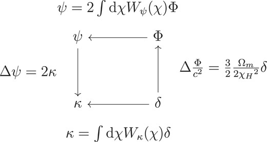
Relationship between density contrast, gravitational potential, lensing potential, and effective convergence.
Our lensing survey parameters are those of a Euclid-like survey. We consider a half-sky survey with fsky = 0.5, a standard deviation of intrinsic ellipticities of galaxies of σϵ = 0.4 and an average number of galaxies per steradian |$\bar{n} = 4.727 \times 10^8$|. Perhaps most importantly, we list results up to a maximum multipole moment of ℓmax = 104. Such a high multipole moment is not accessible in a weak lensing survey. To see the effect of axion DM in the considered mass range, we need to resolve scales at the order of k = 1 h Mpc−1 which roughly corresponds to multipole orders ℓ ≳ 103 in the case of Euclid. In practice, the highest multipole moment measurable in a weak lensing survey is limited by the shape noise. The signal-to-noise ratio of a single-multipole moment drops below 1 at ℓ ∼ 3 × 10³. However, we may still gain information by summing over these noise-dominated multipole moments as we make a relatively conservative estimate for the shape noise. At even higher multipole moments of around ℓ ∼ 5 × 10³, baryonic feedback becomes an important process that is entirely neglected in PT. At this point, our results must become completely unreliable. We still show the plots for multipole moments ℓ ≳ 5 × 10³ to visually compare the different masses.
More importantly, PT disagrees with N-body simulations on the scales considered and significantly underestimates the full non-linearity for large k. We therefore compare with an estimate of the lensing spectrum signal obtained by integrating the power spectra obtained from the L = 30 Mpc h−1N-body simulations from k = 6 h Mpc−1 to k = 30 h Mpc−1 well below the Nyquist frequency |$k_{Nyq} = \pi \frac{N}{L} = 53.6$| h Mpc−1. In addition, we demonstrate how the lensing PT results for CDM and the m = 10−23 eV case change when implementing a hard cut-off on the spectra, that is, we set the input matter spectra to zero above a cut-off scale and study how the PT lensing results depend on the cut-off scale.
3.1 Lensing spectra, bispectra, and trispectra
The angular correlation function for a quantity such as the convergence |$\kappa (\boldsymbol {\theta })$| measured on the sky is given by
where the expectation value is computed as an ensemble average over statistically equivalent realizations of the field |$\kappa (\boldsymbol {\theta })$|. We take the Fourier transform to obtain the angular spectrum in the flat-sky approximation:
To simplify the computation of angular correlation functions, we employ Limber’s approximation (Limber 1953). It asserts that if the quantity |$x(\boldsymbol {\theta })$| defined in two dimensions is a projection
of a quantity |$y(\boldsymbol {r})$| defined in three dimensions with a weight function wx(χ), then the angular spectrum of |$x(\boldsymbol {\theta })$| is given by
where Py(k) is the spectrum of y, evaluated at the three-dimensional wavenumber k = ℓ/χ. This approximation is applicable if y varies on length-scales much smaller than the typical length-scale of the weight function wx. Intuitively, we divide χ by ℓ such that we can compare different scales for a given angle. From the Limber approximation, it immediately follows that the convergence spectrum Cκ(ℓ) is determined by a weighted line-of-sight integral over the spectrum of the density contrast Pδ(k). Likewise, we can express the convergence bi- and trispectrum as appropriately weighted line-of-sight integrals over the bi- and trispectra. All in all, we find
where we introduced the subscripts δ and κ to distinguish between the matter and the convergence spectra. The weight function Wκ is the weak lensing efficiency defined in equation (37). Fig. 9 shows the respective convergence spectra. Non-linear corrections significantly increase the magnitude of the dimensionless spectra for multipole moments ℓ ≳ 100. To highlight where one might expect the models to differ, we translate the comoving quantum Jeans scale into a corresponding multipole order by an order-of-magnitude estimate. We define the quantum Jeans multipole order ℓJ(m) via
where χ(z = z0) is the comoving distance at the redshift z0 and kJ is as defined in equation (13) at z = 99. For the mean redshift z0 = 0.9 of the redshift distribution defined in equation (39), we obtain ℓJ(m = 10−21eV) ≈ 5.0 × 10⁴, ℓJ(m = 10−22eV) ≈ 1.6 × 10⁴ and ℓJ(m = 10−23eV) ≈ 5.0 × 10³. Since these quantum Jeans multipole orders are too high to be measurable in a weak lensing survey, the vertical lines in Fig. 9 display 0.1 × ℓJ which roughly describes the multipole order where the CDM PT and FDM PT lensing spectra start to differ.
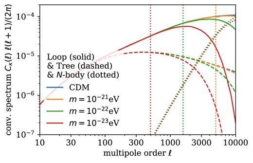
Dimensionless convergence spectra at tree level, with loop-level corrections and from N-body simulations. The N-body results overlap. The vertical, dotted lines correspond to 0.1 × ℓJ where the quantum Jeans multipole order ℓJ is defined in equation (47).
We also compute the lensing spectra using CDM PT with FDM IC via the CDM coupling kernels obtained from the EdS recursion relations as well as the CDM growth factors in the fiducial cosmology. CDM dynamics at tree and loop level yield lensing spectra, bispectra, and trispectra that are, within the numerical errors, indistinguishable from the ones computed using FDM PT. This is why we refrain from showing the corresponding figures. We conclude that the reason for the suppression of the lensing spectra below the quantum Jeans multipole order in PT lies mainly in the ICs and is not the result of the approximation of late-time FDM dynamics through FDM PT.
In contrast, the lensing spectra computed from the N-body spectra in the range k = 6 h Mpc−1 – k = 30 h Mpc−1 paint a different picture. The late-time difference in power on small angular scales between the FDM and CDM models is significantly smaller than estimated via PT. Moreover, the FDM models exhibit more power on small angular scales than predicted via PT. Note that the N-body lensing spectra underestimate power for small ℓ because of the cutoff of k. To assess the impact of the high k-modes of the power spectra estimated via PT, we implement a high-k cutoff in the PT lensing results for CDM and m = 10−23 eV. The tree-level and full loop-level matter power used as input for the lensing integral are set to zero above the cut-off scale. Fig. 10 demonstrates that a significant part of the discerning power of the model survey comes from the modes with k > 3 h Mpc−1. For a smaller cut-off scale, the difference between the CDM and FDM model is not visible and for a cutoff at k = 0.1 h Mpc−1 where the loop-level PT corrections for CDM are highly accurate, even the difference between tree- and loop-level PT is not discernible.
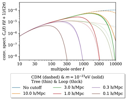
Dimensionless convergence spectra at tree level as well as with loop-level corrections where the loop integrals were evaluated with a small-scale cutoff.

Dimensionless equilateral convergence bispectrum configurations. The vertical, dotted lines correspond to 0.1 × ℓJ where the quantum Jeans multipole order ℓJ is defined in equation (47).
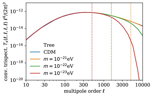
Dimensionless equilateral square convergence trispectrum configurations. The vertical, dotted lines correspond to 0.1 × ℓJ where the quantum Jeans multipole order ℓJ is defined in equation (47).
3.2 Attainable signal strength
The convergence spectrum is measured by analysing the ellipticities of an ensemble of galaxy images. Averaging over N faint galaxy images, the scatter of the intrinsic ellipticity is reduced to
where σϵ is the standard deviation of the intrinsic ellipticity. The angular resolution of this measurement is limited by
where |$\bar{n}$| is the average number of source galaxies per squared arc minute. As a result, the observed convergence spectrum |$C_{\kappa }^{(\mathrm{obs})}(\ell)$| can be modelled as the true spectrum with an additional shot noise contribution:
Assuming that the estimates for the spectra can be approximated by a Gaussian distribution, we can estimate the covariance matrices for the lensing spectra, bispectra, and trispectra. The covariance of the lensing spectrum is given by
where fsky denotes the fraction of the observed sky and we neglect a contribution proportional to the lensing trispectrum due to the non-Gaussianity of the weak lensing field (Kaiser 1998; Scoccimarro, Zaldarriaga & Hui 1999). Takada & Jain (2004) provide an expression for the covariance of the weak lensing bispectrum:
where ℓi ≤ ℓi + 1 to count every triangle/quadrilateral configuration only once. Δ(ℓ1, l2, l3) counts the multiplicity of triangle configurations and is defined as
Similarly, we have
for the covariance of the weak lensing trispectrum where Δ(ℓ1, ℓ2, ℓ3, ℓ4) counts the multiplicity of quadrilateral configurations. These covariance matrices allow us to understand the statistical uncertainties of the spectrum measurement. With their help, we can calculate the expected cumulative signal-to-noise ratio Σ(ℓ) for weak lensing measurements of the different spectra up to multipole order ℓ:4
Fig. 13 shows the signal-to-noise ratios obtained in CDM according to equations (55), (56), and (57). We compute the respective covariance matrices using the convergence spectrum with loop-level corrections. This is because the non-vanishing contributions to the bi- and trispectra are generated by non-linear dynamics. Using the tree-level convergence spectra would therefore underestimate the covariance and overestimate the attainable signal-to-noise ratios. Since the bulk of the cumulative signal comes from the modes with low ℓ, there are no significant differences in the attainable signal-to-noise ratios in CDM and FDM weak lensing surveys for the considered masses. We do not show the respective N-body results since they would severely underestimate the attainable S2N ratios due to the finite box size. The sums in equations (55), (56), and (57) are expressed as integrals and integrated using the cuba library (Hahn 2005). The signal-to-noise ratios for the weak lensing bispectra at loop level for FDM proved computationally intractable.
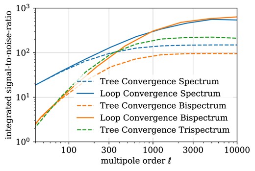
Attainable signal-to-noise ratio for convergence spectra at tree and loop level, convergence bispectra at tree and loop level and convergence trispectra at tree level (CDM and FDM identical).
Nevertheless, we compare against the signal-to-noise ratios of the loop-level lensing bispectra computed with CDM PT for FDM IC. Note, however, that these results are also subject to substantial numerical uncertainty since the Monte Carlo integration routine fails to provide error estimates. Fig. 14 visualizes the angular dependence of the lensing bispectrum at tree level for m = 10−23 eV. The bottom plots reflect that the small-angular scales where the CDM and FDM models differ only have a relatively small signal-to-noise ratio in a weak lensing survey. In contrast, Fig. 15 shows the corresponding loop-level results approximated by CDM with FDM IC. We observe that the loop-level corrections significantly enhance the signal-to-noise ratio for the multipole orders where CDM and FDM with m = 10−23 eV can be distinguished.
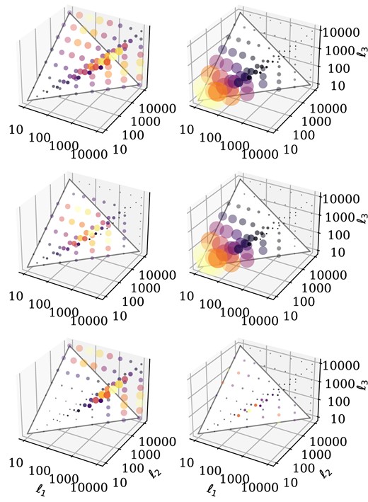
Configuration dependence (first column) and signal-to-noise ratio (second column) of the weak lensing bispectrum at tree level. Colour and size both represent magnitudes. Same, arbitrary normalization is employed across rows. Top to bottom: CDM, FDM for m = 10−23 and the difference between the two. Left column: Dimensionless lensing bispectrum |$(\ell _1\ell _2\ell _3)^{\frac{3}{4}}B_{\kappa }(\ell _1, \ell _2, \ell _3)$| at z = 0. Right column: Signal-to-noise ratio |$B_{\kappa }(\ell _1, \ell _2, \ell _3)/\sqrt{\text{cov}(\ell _1, \ell _2, \ell _3)}$| at z = 0.

Configuration dependence (first column) and signal-to-noise ratio (second column) of the weak lensing bispectrum at loop level where FDM dynamics are approximated by CDM PT with FDM IC. Colour and size both represent magnitudes. Same normalization as in Fig. 14. Top to bottom: CDM, CDM with FDM IC for m = 10−23 and the difference between the two. Left column: Dimensionless lensing bispectrum |$(\ell _1\ell _2\ell _3)^{\frac{3}{4}}B_{\kappa }(\ell _1, \ell _2, \ell _3)$| at z = 0. Right column: Signal-to-noise ratio |$B_{\kappa }(\ell _1, \ell _2, \ell _3)/\sqrt{\text{cov}(\ell _1, \ell _2, \ell _3)}$| at z = 0.
3.3 Differentiability between FDM and standard CDM
We can also give an estimate of whether we can distinguish CDM and FDM experimentally via a weak lensing survey. We assume that the true spectra are given by the CDM spectra and compute the χ2-functionals for measuring the noise-weighted mismatch between the true CDM and the wrongly assumed FDM spectra:
Fig. 16 shows the χ2-functionals for distinguishing CDM and FDM computed according to equations (58) and (59) where all sums are again expressed as integrals and calculated using the cuba library (Hahn 2005).
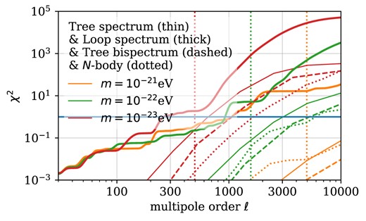
Differentiability between CDM and FDM in terms of the χ2-functionals for weak lensing spectra and bispectra as a function of the maximum multipole order ℓ according to equations (58) and (59). The vertical, dotted lines correspond to 0.1 × ℓJ where the quantum Jeans multipole order ℓJ is defined in equation (47). The horizontal blue line corresponds to χ2 = 1.
We observe that the χ2-values obtained from the N-body simulation for a box size of L = 30 Mpc h–1 for k between 6 h Mpc−1 and 30 h Mpc−1 are significantly lower than the PT predictions at loop and even at tree level. While we expected linear PT to provide a conservative estimate of the distinguishing power of the model lensing survey, it seems that the restoration of small-scale power through late-time non-linear CDM dynamics might cause the actual signal to be smaller than predicted by PT. Further contrasting FDM PT and CDM PT in Fig. 17, we conclude that the difference in late-time dynamics between FDM and CDM is negligible for the χ2-values computed via PT. The only obvious difference at high ℓ arises for the m = 10−21 eV loop-level PT prediction. Since the other spectra agree well and the FDM PT loop-level PT lensing prediction is computed using splines, we conclude that the respective FDM PT χ2 functional is dominated by noise up to high ℓ. Fig. 18 displaying the tree level χ2-functionals for FDM PT and CDM PT with FDM IC underscores this conclusion.
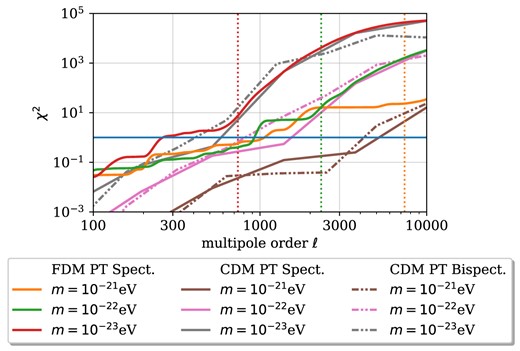
Differentiability between CDM and FDM in terms of the χ2-functional for weak lensing spectra and bispectra as a function of the maximum multipole order ℓ according to equations (58), (59), and (60). Both FDM PT and FDM dynamics approximated by CDM PT with FDM IC are shown. The vertical, dotted lines correspond to 0.1 × ℓJ where the quantum Jeans multipole order ℓJ is defined in equation (47).
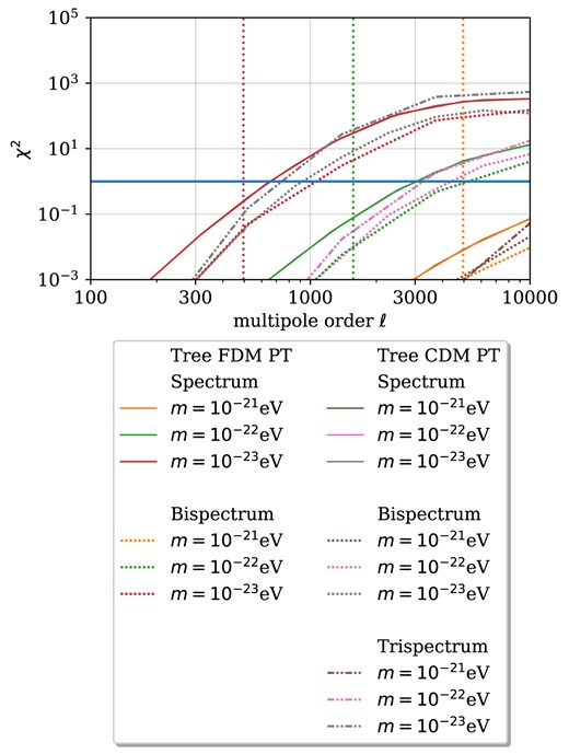
Differentiability between CDM and FDM in terms of the χ2-functional for weak lensing spectra, bispectra, and trispectra as a function of the maximum multipole order ℓ according to equations (58), (59), and (60). Both FDM PT and FDM dynamics approximated by CDM PT with FDM IC are shown. The vertical, dotted lines correspond to 0.1 × ℓJ where the quantum Jeans multipole order ℓJ is defined in equation (47).
4 SUMMARY AND DISCUSSION
In this work, we studied structure formation in the CDM and FDM models and their possible distinction through a Euclid-like weak lensing survey. We extended Eulerian PT to account for genuine quantum mechanical effects on the de Broglie scale of the dark matter particle. For sufficiently light elementary particles, such as axions and axion-like particles, this scale can be set to be relevant for cosmological structures on the scale of galaxies and below, typically for masses in the range of 10−23… − 21 eV. As a consequence of the Madelung transform of the Schödinger equation, the fluid mechanical equations acquire a quantum pressure term, counteracting structure formation on scales smaller than the de Broglie scale. We draw the following conclusions:
Evolving the density and velocity fields using Eulerian PT including a quantum pressure term with suitable Gaussian ICs leads us to perturbative expressions for the bi- and trispectra, as well as non-linear corrections to the spectra themselves. We can consistently compute corrections to the spectra and the bispectra at loop level using FDM PT and CDM PT with FDM IC. Limitations in the numerical evaluation of the resulting integrals via adaptive integration schemes restrict us to tree-level evaluation of the trispectra. In all computations, non-linear structure formation as predicted by PT does not make up for the lack of initial power on small scales. In contrast, small-scale power on mildly non-linear scales is almost completely restored according to the N-body prediction. In both CDM and FDM, non-linear effects lead to increased spectral amplitudes on scales larger than the de Broglie scale.
Limber projection in the flat-sky approximation with lensing efficiency functions incorporating a Euclid-like source redshift distribution yields lensing spectra, bispectra, and trispectra. Again, the lensing quantities are evaluated using adaptive integration. We choose lensing as an observational channel to be independent of any biasing assumption typical for galaxy surveys. The respective shear spectra can be found through a correlation analysis of galaxy shapes. As expected, we find a loss in power on the de Broglie scale in the FDM models compared to the CDM model. However, the loss of power predicted by the N-body simulations is significantly smaller than the loss of power predicted by FDM PT. For reference, we convert the de Broglie scale into an angular scale with a typical comoving distance corresponding to the median redshift. Measurements of bi- and even trispectra are clearly within reach of Euclid, with a significance of a few hundred σ: In these estimates, we use a full configuration and scale integration with shape noise and a non-linear covariance.
With a similar numerical computation, we can estimate whether the spectra, bispectra, and trispectra for the CDM and FDM cases are distinguishable: For this purpose, we compute the χ2-functional for a given Gaussian-approximated non-linear CDM covariance as a function of the FDM particle mass. As in the case of the signal-to-noise computations, the χ2-functionals follow from a complete configuration space integration up to a limiting multipole, and we consider Δχ2 = 1 as a rough criterion of distinguishability: For FDM at tree level with m = 10−23 eV this limit is reached at ℓ ∼ 700. The N-body lensing prediction indicates that this limit is reached at ℓ ∼ 1000 − 2000. Yet, for m = 10−23 eV the late-time impact of the quantum pressure on the scales considered is non-negligible which is why this result suffers from a substantial uncertainty. For masses m = 10−22 eV and m = 10−21 eV, the respective signals in our weak lensing survey are too weak to distinguish CDM and FDM below ℓ = 3 × 10³. This is the maximum multipole order accessible in a Euclid-like survey. The lensing bispectrum gives a lower χ2-functional than the lensing spectrum at tree level, but might still serve as an important cross-validation.
CDM loop-level perturbative results are found to agree reasonably well with the CDM N-body predictions while FDM loop-level PT significantly underestimates the power on scales k ∼ 1 − 100 h Mpc−1 when compared to the N-body predictions. Unless the additional suppression of small-scale power through late-time FDM dynamics significantly increases the values of the χ2-functionals, the values χ2 = 1 at ℓ ∼ 600 and ℓ ∼ 1500 for m = 10−23 eV and m = 10−22 eV by the loop-level lensing spectra are found to be unreliable. In any case, the signal for m = 10−21 eV is still too weak to be measurable in a realistic weak lensing survey. Considering PT at loop level, the lensing bispectrum gives slightly higher χ2-values than the lensing spectrum. Again, these values are likely unreliable and overestimate the potential of a Euclid-like weak lensing survey.
The main uncertainty in our approach stems from the modelling of non-linear structure formation via PT. In general, the extent to which the FDM and CDM models can be compared depends on the times and scales considered. As the analysis of the impact of a high-k cutoff on the loop-level matter power spectra demonstrates, the bulk of the lensing signal comes from modes with k > 3 h Mpc−1 for all masses considered. At these scales, loop-level PT is known to underestimate the true power spectra at late times. However, as the comparison with the N-body simulations highlights, full non-linear CDM dynamics make up for the initial lack of small-scale power while loop-level PT does not. As a consequence, PT seems to significantly overestimate the attainable χ2-functionals and is therefore not the right tool to distinguish between the considered FDM models and the CDM model in our weak lensing survey. Still, PT might be suited for other observational channels, such as neutral hydrogen surveys for probing the cosmic dawn. They are confined to probing the cosmic state before reionization at z ∼ 6 where PT still provides a better estimate for the non-linearity at smaller scales. Technical and numerical details of the FDM PT are described in detail in Appendices A – C, along with the representation of the coupling kernels in terms of Feynman diagrams.
The estimation of the power spectra from N-body simulations is subject to several uncertainties: We only run one simulation per box size and IC. Ideally, one conducts a statistically representative sample of simulations with different ICs and averages over the resulting spectra to obtain error estimates. The large-scale power suffers estimated from runs in small simulation volumes is underestimated and suffers from high variance due to a lack of samples. Most importantly, a consistent FDM simulation in a sufficiently large simulation box would be required to reliably estimate the late-time power spectrum on small scales and, as a consequence, the lensing spectra for the FDM masses m = 10−22 eV and m = 10−23 eV considered here.
Acknowledgement
We would like to thank Guan-Ming Su for providing power spectra from numerical FDM simulations to crosscheck the perturbation theoretical results. This work made significant use of many open-source software packages, including python, ipython, numpy, scipy, matplotlib, yt, cuba, and gsl. These are products of collaborative efforts by many independent developers from numerous institutions around the world. Their commitment to open science has helped to make this work possible.
DATA AVAILABILITY STATEMENT
The code that computes the matter spectra, bispectra, and trispectra in CDM and FDM is available under https://github.com/KunkelAlexander/fdm-eulerpt.
Footnotes
Note, however, that in the context of axion cosmology, the quantum pressure follows from the non-relativistic equation of motion of a classical field and is therefore not a quantum mechanical result.
Note that a consistent truncation of series in PT is obtained by including terms up to a certain power m in the linear spectrum. This corresponds to grouping the PT contributions in terms of the number of loops in a diagrammatic representation.
We were unable to compute the PT kernels in a general cosmology in FDM. This would require obtaining two linearly independent solutions to the linear growth equation equation (15).
Note that unlike for lensing bispectrum configurations that are uniquely specified by the three multipole moments ℓ1, ℓ2, ℓ3 up to spatial orientation, a lensing trispectrum configuration is not uniquely specified by ℓ1, …, ℓ4. In our code, we sum over all configurations by varying the length of three sides as well as the two enclosed angles.
References
APPENDIX A: TIME-DEPENDENT PT
In this section, we develop a general framework for time-dependent Eulerian PT that we then apply to FDM. The CDM case follows by setting ℏ = 0, that is, the formal transition from quantum to classical mechanics. We start with a system of two coupled equations of the form
where |$\nabla \cdot \boldsymbol {\upsilon } = \theta$|, f is a well-behaved function that is allowed to depend on θ and δ and their spatial derivatives and we work in the conformal time τ. Hence, equation (A2) includes both the ideal fluid equations with pressure if we neglect the vorticity degrees of freedom as well as the Madelung equations. In the latter case, f(θ, δ) includes the full non-linear quantum pressure term. By later expanding this expression in terms of the density contrast δ and truncating the resulting series at a given order in δ, we perturbatively include the effects of the non-linearities of the quantum pressure. Further, we introduce the two-component vector
such that the density and velocity fields can be treated on equal footing. We now expand equation (A2) in terms of powers of δ and θ and then Fourier transform it:
where we introduced the time- and scale-dependent mode-coupling matrices Ωab and |$\Gamma _{a, i_1,\ldots ,i_n}$| for the indices a, b, i1, …, in ∈ {1, 2} and we employ the Einstein sum convention. Moreover, we employ a convention where integration over momenta |$\boldsymbol {k}_i, \boldsymbol {k}_j$| with equal indices i, j is understood:
The matrix Ωab encodes the linearized fluctuations, whereas the matrices |$\Gamma _{a, i_1\ldots i_n}$| encode all non-linearities. The meaning of the indices can be easily understood: The index a tells us whether we are looking at a contribution to the density contrast δ or the velocity divergence θ. The indices i tell us which fields couple to one another. The continuity equation equation (A1) gives Ω11 = 0 and Ω12 = 1. We can therefore substitute
into equation (A2) for a = 2 to obtain
where we omit the time and momentum variables. The inhomogeneity |$g(\boldsymbol {k}, \tau)$| is defined as
Linearizing equation (A7) gives the homogeneous, linear second-order ODE
whose solutions are the linear growth factors D+ and D− if we make the ansatz |$\Psi _1^{(1)}(\boldsymbol {k}, \tau) = \delta (\boldsymbol {k}, \tau _0) D(\tau , \tau _0)$|. A particular solution of an inhomogeneous second-order ODE can be found by the convolution of the inhomogeneity g(k, a) with the Green’s function Gk(s, a):
where the Green’s function Gk(s, τ) of the ODE is given by a combination of two linearly independent solutions, that is, D+ and D−, of the homogeneous equation
The Green’s function has the following properties:
The crucial idea of the derivation of the coupling kernels is as follows: Writing down the convolution in equation (A10) for the inhomogeneity defined in equation (A8), one obtains an integral equation for Ψa. This integral equation can be brought into the form of equations (23) and (24). Finding the coupling kernels Fi and Gi then boils down to comparing integrands. Pursuing this idea, we express the solution Ψ1 of the full theory as sum of the homogeneous solution |$\Psi ^{(1)}_1$| and a particular solution
We now parametrize the inhomogeneous solution in terms of the vertex couplings |$C^{(n)}_{a, i_1\ldots i_n}(\boldsymbol {k}, \boldsymbol {k}_1, \ldots , \boldsymbol {k}_n, s, \tau)$| and write
The vertex couplings for Ψ1 can be immediately derived from equation (A8) by partial integration of the derivative term |$\partial _{s} \bigl [\Gamma _{1,i_1\ldots i_n} \Psi _{i_1}(\boldsymbol {k}_1, s) \times \ldots \times \Psi _{i_n}(\boldsymbol {k}_n, s)\bigl ]$| using Gk(τ, τ) = 0:
The vertex couplings C(n) owe their name to the diagrammatic representation of equation (A13) shown in Fig. A1. In the following, we make use of this diagrammatic language to compute the higher-order coupling kernels. Equation (A13) can be used to obtain the perturbative solution iteratively: We substitute |$\Psi = \Psi ^{(1)} + \mathcal {O}(\delta ^2, \upsilon ^2, \delta \upsilon)$| into the RHS of equation (A13) which gives an equation whose solution is Ψ = Ψ(1) + Ψ(2) + third-order terms. Substituting this expression back into the RHS of equation (A13) gives an equation whose solution is Ψ = Ψ(1) + Ψ(2) + Ψ(3) + fourth-order terms and so on. The following section gives expressions for |$\Psi _a(\boldsymbol {k}, \tau)$| up to quartic order to compute the kernels F2, F3 and F4. The linear velocity divergence fluctuations are related to the density fluctuations via
We therefore define the two-component vector |$\boldsymbol {f}$| that relates the linear density and velocity divergence fluctuations at time s with the linear density fluctuations at time τ:
With this definition in place, |$\Psi _a^{(2)}(\boldsymbol {k}, \tau)$| can be expressed as
Comparing this expression to the definition of Fn in equation (23), we can finally read off the coupling kernels. The coupling kernel F2 can be expressed diagrammatically as shown in Fig. A2 or explicitly written as
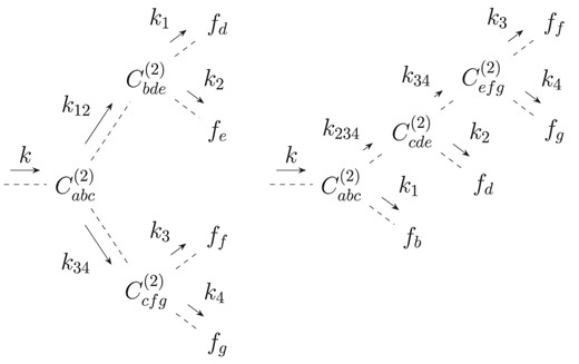
Note that all the kernels derived in this section have yet to be symmetrized with respect to exchange of momenta. We now proceed by deriving the kernels at third and fourth order in diagrammatic representation. At third order, the diagrammatic representation of the coupling kernels F3 and G3 is given by the two types of diagrams shown in Fig. A3. Finally, at fourth order, we find the diagrams shown in Figs A4, A5, and A6.
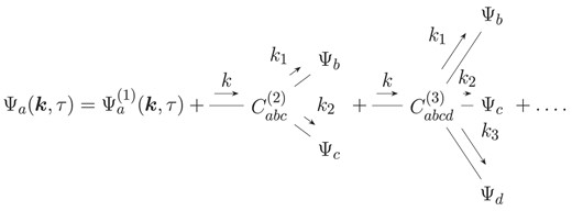
Diagrammatic representation of equation (A13) in terms of trees. Outgoing momentum arrows express momentum integrations. The Dirac-Delta functions enforce momentum conservation at the vertices and employ the Einstein sum convention for repeated indices. The depth of the tree denotes the number of time integrations.
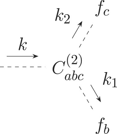
Diagrammatic representation of the coupling kernels F2 and G2. There is one free index a that describes the density coupling kernel |$F_2(\boldsymbol {k}, \boldsymbol {k}_1, \boldsymbol {k}_2)$| for a = 1 and the velocity coupling kernel |$G_2(\boldsymbol {k}, \boldsymbol {k}_1, \boldsymbol {k}_2)$| for a = 2. The tree has a depth of one and therefore requires one time integration.
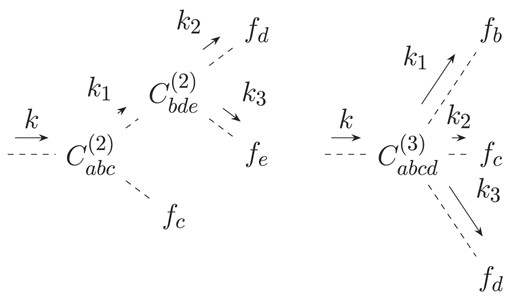
Diagrammatic representation of contributions to PT kernels F3 and G3. The left diagram describes two contributions with the permutation b↔c. The depth of the tree is 2. Accordingly, it requires two time integrations.
Diagrammatic representation of contributions to PT kernels F4 and G4 involving only the fourth-order vertex coupling C(4).
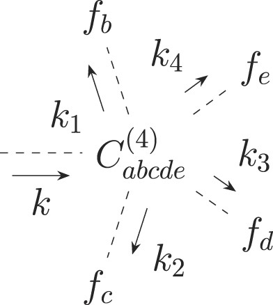
Diagrammatic representation of contributions to PT kernels F4 and G4 involving only the second-order vertex coupling C(2). There are four additional permutations: the permutation b↔c for the left diagram as well as three additional permutations b↔c and d↔e for the right diagram.
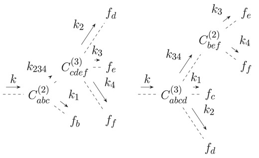
Diagrammatic representation of contributions to PT kernels F4 and G4 involving both the second-order and third-order vertex couplings C(2) and C(3). There are three additional permutations: the permutation b↔c for the left diagram and two additional permutations b↔c↔d for the right diagram.
A1 FDM for EdS cosmology
We now apply the time-dependent PT framework to the FDM case. First, we review the Madelung equations (8) in terms of the conformal time τ
Secondly, we Fourier transform the Madelung equations. The Fourier transform of the quantum pressure term is computed by the Taylor expansion up to eighth order using Mathematica (Wolfram Research 2021). We obtain the same continuity equation as in the CDM case:
as well as the Euler equation with quantum-pressure corrections
where we omitted the time dependence of all quantities and integrations over momenta with repeated indices are understood. Comparing equations (A23) and (A24) to equation (A4), we can now determine the mode coupling matrices. Following the convention in (Li, Hui & Bryan 2019) we provide them in terms of the time |$\eta \equiv 2 \sqrt{a} = H_0 \tau$|. The linear mode coupling matrix Ωab reads
where the characteristic FDM scale b(k) is defined as
Ω21 vanishes when k equals the comoving quantum Jeans scale kJ. We compute the non-linear mode coupling matrices |$\Gamma _{a, i_1, \ldots , i_n}$| up to n = 4: At second order, the matrices |$\Gamma _{a,i_1, i_2}$| include the non-linear contribution from the convection term as well as the second-order mode coupling from the quantum pressure term:
where |$\alpha (\boldsymbol {k}, \boldsymbol {k}_1)$| and |$\beta (\boldsymbol {k}, \boldsymbol {k}_1, \boldsymbol {k}_2)$| are defined as
and all other components vanish. All higher-order contributions to |$\Gamma _{a, i_1\ldots i_n}$| stem solely from the quantum pressure term and therefore represent self-interactions of the density field:
and all other contributions at third and fourth order vanish. Using the analytical growth factors given in equation (19), we find the Green’s function
Note that the Green’s function is free of divergences because the denominators of the growth functions at the initial time cancel. Using equation (A14), the vertex couplings are given by
at second order as well as
at third and fourth order where all other vertex couplings vanish. This is because above order two there are only self-interactions of the density field stemming from the Taylor expansion of the quantum pressure term. This simplifies the computation and the symmetrization of the kernels |$F_3^{FDM}$| and |$F_4^{FDM}$| significantly. A more detailed discussion can be found in Appendix B.
Since |$\gamma _{abc}(\boldsymbol {k}, \boldsymbol {k}_1, \boldsymbol {k}_2, s, \eta)$| is symmetric with respect to exchange of |$\boldsymbol {k}_1$| and |$\boldsymbol {k}_2$|, |$C^{(2)}_{1bc}(\boldsymbol {k}, \boldsymbol {k}_1, \boldsymbol {k}_2, s, \eta)$| inherits this property. As a consequence |$F_2^{FDM}$|, as given by equation (A19), is already symmetric under the exchange of the momenta |$\boldsymbol {k}_1$| and |$\boldsymbol {k}_2$|.
APPENDIX B: EXPLICIT SYMMETRIZATION OF FDM PT KERNELS
In this section, we explicitly derive the symmetrized FDM PT kernels |$F_3^{(s)}$| and |$F_4^{(s)}$| by making use of the symmetries of the vertex couplings in FDM. We start with the third-order kernel F3 depicted in Fig. A3. It can be explicitly expressed as |$F_3 = I^{(3)}_1 + J^{(3)}_1$| with
Since Γ1bc = Γ1cb, as follows from equation (A27), equation (B1) reduces to
Since |$I^{(3)}_1$| already enjoys symmetry under |$\boldsymbol {k}_2 \leftrightarrow \boldsymbol {k}_3$| and |$\boldsymbol {k}_{23} \leftrightarrow \boldsymbol {k}_1$|, it can be symmetrized as
Furthermore, |$J^{(3)}_1$| is already symmetric under the exchange of momenta because the only non-vanishing element of the vertex coupling Γ at fourth order is the (1111)-component given in equation (A30) that stems from the quantum pressure term and is already symmetric under the exchange of momenta |$J^{(3, s)}_1(\boldsymbol {k}_1, \boldsymbol {k}_2, \boldsymbol {k}_3, \eta) = J^{(3)}_1(\boldsymbol {k}_1, \boldsymbol {k}_2, \boldsymbol {k}_3, \eta)$|. We conclude |$F_3^{(s)} = J^{(3, s)}_1(\boldsymbol {k}_1, \boldsymbol {k}_2, \boldsymbol {k}_3, \eta) + I^{(3,s)}_1(\boldsymbol {k}_1, \boldsymbol {k}_2, \boldsymbol {k}_3, \eta)$|. At fourth order, we distinguish five contributions to the coupling kernel:
The contribution W4 corresponds to the diagram in Fig. A4 and takes the simple form
Like in the third-order case, |$\Gamma ^{(4)}_{11111}$| stems from the quantum pressure term and is therefore symmetric under the exchange momenta. As a consequence W4 is symmetric under the exchange of momenta. The contribution I4 corresponds to the left diagram in Fig. A5:
which can be symmetrized by using the fact that it is already invariant under |$\boldsymbol {k}_1 \leftrightarrow \boldsymbol {k}_2$|; |$\boldsymbol {k}_3 \leftrightarrow \boldsymbol {k}_4$|; |$\boldsymbol {k}_1 , \boldsymbol {k}_2 \leftrightarrow \boldsymbol {k}_3, \boldsymbol {k}_4$|:
The contribution J4 corresponds to the right diagram in Fig. A5:
and enjoys symmetry under |$\boldsymbol {k}_1 \leftrightarrow \boldsymbol {k}_{234}$|; |$\boldsymbol {k}_2 \leftrightarrow \boldsymbol {k}_{34}$|; |$\boldsymbol {k}_{3} \leftrightarrow \boldsymbol {k}_4$|. The factor 4 follows from the three additional permutations of the diagram. Its fully symmetric form is given by
The contribution K4 corresponds to the left diagram in Fig. A6:
where the additional permutation together with the symmetry properties of |$\Gamma ^{(2)}_{abc}$| give the factor of 2. Again, we recognize that the expression is invariant under permutations of |$\boldsymbol {k}_2, \boldsymbol {k}_3$| and |$\boldsymbol {k}_4$|. Its symmetric form is given by
The last remaining contribution H4 corresponds to the right diagram in Fig. A6:
A symmetrized form of H4 is given by
It follows that
APPENDIX C: COMPUTATION OF LENSING INTEGRALS
In the following, we describe how to perform the loop-level, line-of-sight, signal-to-noise and χ2 integrations. First, we consider the numerical loop-level integrations to the matter spectra. The relevant integrals are given by equations (27) and (31). Both integrands exhibit IR divergences. Carrasco et al. (2013) argue that if one succeeds in rewriting the integrands such that the leading IR divergences cancel, all subleading IR divergences are guaranteed to cancel as well. They provide such an expression for the power spectrum:
Equation (C1) can be applied to the FDM case since the momentum dependence of the FDM mode coupling functions does not introduce any additional divergences compared to the CDM case. The same holds true for the IR-safe version of the bispectrum corrections that are divergent just as in the case of the one-loop power spectrum.
Baldauf et al. (2014) provide an IR-safe expression for the bispectrum contributions: The integrands of the contributions |$B_{321}^{II}$| and B411 as defined in equation (31) only exhibit divergences at q = 0. The integrand of |$B_{321}^{II}$| exhibits a divergence at |$\boldsymbol {q} = \boldsymbol {k}_2$| which can be mapped to a divergence at q = 0 by writing
Similarly, one finds the following expression for the integrand of B222:
The full one-loop bispectrum in a form where all IR divergences cancel is then given by
We integrate the above expressions for the IR-safe loop-level corrections to the matter power spectrum and bispectrum using the cuba library (Hahn 2005). For the loop-level corrections to the CDM power spectrum, the four integration algorithms Vegas, Cuhre, Divonne, and Suave all provide good results. The FDM integrations are much more problematic because they involve time integrations for the PT kernels in addition to the momentum integrations. In addition, the PT kernels and the growth factor both exhibit strong oscillations for large k. As a consequence, integrations take as long as 5 CPU hours for the Monte Carlo integration of the one-loop contribution to the FDM bispectrum for a single triangle configuration with a relative error of 10 per cent. For computing the power spectrum loop-level corrections, we use the Vegas algorithm that stores the integrand structure between different integration runs and thus accelerates integration for different k values. For the bispectrum loop-level corrections, we use the Divonne algorithm. We test our integration routines by comparing their results with the analytical solutions in the CDM case derived by Makino, Sasaki & Suto (1992). Furthermore, we numerically verify that the FDM PT kernels reduce to the correct analytical CDM expressions for small k. Moreover, we implement the PT code independently in python and C++ and crosscheck the results.
For the numerical integration of the line-of-sight integrals, we combine the PT kernel integrations, the loop integrations and the line-of-sight integrations into higher dimensional integrals that we integrate using the cuba library. This proves advantageous since the line-of-sight integrations smooth out oscillations and make the loop integrations more numerically tractable. The signal-to-noise sums and χ2-functionals are also computed as integrals using the cuba library. This leads to difficulties during the evaluation of the FDM loop-level bispectrum signal-to-noise sums and χ2-functionals. The combination of the six-dimensional PT integrals to compute the lensing bispectra and the line-of-sight integral yields a seven-dimensional integral. The computation of a single loop-level signal-to-noise ratio therefore requires the evaluation of a three-dimensional integral of a seven-dimensional integral which is computationally intractable. As an alternative, we combine the signal-to-noise integrals and the PT integrals to obtain a seventeen-dimensional integral which again proves computationally intractable. In the CDM case, this approach works better and yields an eleven-dimensional integral that can be evaluated numerically. We use this approach to estimate the loop-level bispectrum signal-to-noise ratios and χ2-functionals.
APPENDIX D: N-BODY SIMULATIONS
We run a total of 8 simulations with N = 5123 particles with the box sizes L = 30 Mpc h−1 and L = 256 Mpc h−1. They serve as an estimate of the full non-linear evolution of the CDM and FDM models. The ICs are created from the respective CAMB and axionCAMB spectra using the IC generator music (Hahn & Abel 2011). The simulations themselves are run from z = 99 to z = 0 with a total of 99 snapshots and a comoving gravitational softening length of 14 kpc h−1 and 1.7 kpc h−1, respectively. We use the tool GenPK to compute the matter power spectra from the snapshots (Bird 2017). The lensing spectra are integrated using a 2D spline fitted to the matter spectra in time and k-space. Fig. D1 shows the mass projections of the simulations used for the lensing predictions. The m = 10−23 eV plot in the lower right corner highlights another problem that N-body simulations with suppressed small-scale initial power suffer from: the formation of spurious haloes arranged like beads on a string along the filaments (for instance, see (Schive et al. 2016) for more information). These spurious collapsed objects likely also lead to an overestimation of small-scale power at late times in the N-body runs.
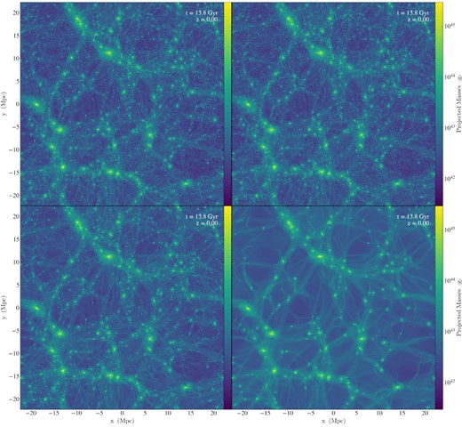
Mass projections of N-body simulations for CDM (upper left) and FDM IC with m = 10−21 eV (upper right), m = 10−22 eV (lower left), and m = 10−23 eV (lower right) in a L = 30 Mpc h−1 box with 5123 particles at z = 0.
