


ABSTRACT
In this paper, we study six slowly rotating mid-to-late M dwarfs (rotation period |$P_{\mathrm{rot}}\approx 40-190\, \mathrm{d}$|) by analysing spectropolarimetric data collected with SpectroPolarimetre InfraRouge (SPIRou) at the Canada–France–Hawaii Telescope as part of the SPIRou Legacy Survey from 2019 to 2022. From ≈100–200 least-squares-deconvolved (LSD) profiles of circularly polarized spectra of each star, we confirm the stellar rotation periods of the six M dwarfs and explore their large-scale magnetic field topology and its evolution with time using both the method based on principal component analysis (PCA) proposed recently and Zeeman–Doppler imaging. All M dwarfs show large-scale field variations on the time-scale of their rotation periods, directly seen from the circularly polarized LSD profiles using the PCA method. We detect a magnetic polarity reversal for the fully convective M dwarf GJ 1151, and a possible inversion in progress for Gl 905. The four fully convective M dwarfs of our small sample (Gl 905, GJ 1289, GJ 1151, and GJ 1286) show a larger amount of temporal variations (mainly in field strength and axisymmetry) than the two partly convective ones (Gl 617B and Gl 408). Surprisingly, the six M dwarfs show large-scale field strengths in the range between 20 and 200 G similar to those of M dwarfs rotating significantly faster. Our findings imply that the large-scale fields of very slowly rotating M dwarfs are likely generated through dynamo processes operating in a different regime than those of the faster rotators that have been magnetically characterized so far.
1 INTRODUCTION
M dwarfs are known to host strong magnetic fields with large- and small-scale field strengths that may exceed 1 kG (Morin et al. 2010; Kochukhov 2021). Zeeman–Doppler imaging (ZDI; Donati & Brown 1997; Donati et al. 2006) revealed different types of large-scale field topologies for M dwarfs: the partly convective early M dwarfs usually showing more complex, relatively weaker fields with non-axisymmetric poloidal fields and significant toroidal components (Donati et al. 2008). Mid M dwarfs often display simpler and stronger, mainly poloidal and axisymmetric large-scale fields (Morin et al. 2008) whereas the fully convective late M dwarfs of lowest masses may end up showing large-scale fields in either configuration (Morin et al. 2010; see also the review by Donati & Landstreet 2009).
Besides, magnetic activity (diagnosed by various proxies) increases for shorter rotation periods until it saturates, i.e. no longer increases with decreasing rotation periods (see e.g. Saar 1996; Wright et al. 2011). In the unsaturated regime, both large- and small-scale fields, diagnosed by polarized and unpolarized Zeeman signatures on line profiles, increase with decreasing rotation periods (Vidotto et al. 2014; See et al. 2015; Reiners et al. 2022).
The main parameter that describes magnetic fields and activity of most M dwarfs is found to be the Rossby number Ro, equal to the rotation period divided by the convective turnover time (e.g. Noyes et al. 1984; Wright et al. 2018, and references therein), with magnetic fields and activity increasing with decreasing Ro until saturation occurs at Ro ∼ 0.1 and below. Whereas large-scale fields of M dwarfs featuring Ro < 1 have been extensively studied, very little is known about those of very slow rotators with Ro ∼ 1 or larger.
In this paper, we explore large-scale fields of a small sample of very slowly rotating M dwarfs, whose fields and rotation periods were inaccessible to optical instruments. The six M dwarfs were observed with the SpectroPolarimetre InfraRouge (SPIRou), the near-infrared spectropolarimeter and velocimeter recently mounted on the Canada–France–Hawaii Telescope (CFHT), in the framework of the SPIRou Legacy Survey (SLS; Donati et al. 2020). The SLS is a large programme carried out with SPIRou at CFHT from early 2019 to mid 2022, with a 310-night time allocation spread over this period. The two main goals of the SLS are (i) the search for habitable Earth-like planets around very low mass stars and (ii) the study of low-mass star and planet formation in the presence of magnetic fields. Its long timeframe (of seven semesters) enables us to investigate the temporal variability in the time series of the monitored M dwarfs, and in particular to independently estimate rotation periods of up to a few hundred days and to study the temporal evolution of their large-scale magnetic fields (Bellotti et al. 2023; Donati et al. 2023, hereinafter D23; Fouqué et al. 2023).
In Section 2, we will present the details of the observations and targets. To analyse the magnetic field properties and to determine the stellar rotation period, we use different methods explained in Section 3, before we present our results for each M dwarf individually in Sections 4–9. We conclude and discuss our results in Section 10.
2 SPIROU OBSERVATIONS
We analyse here a total of 986 circularly polarized spectra collected with SPIRou. The spectra span a wavelength range of 0.95–2.5 μm in the near-infrared with a resolving power of |$R=70\, 000$|. Further details about SPIRou and its spectropolarimetric capabilities can be found in Donati et al. (2020). To process the data, we used the new version of libre esprit, i.e. the nominal reduction pipeline of ESPaDOnS at CFHT optimized for spectropolarimetry and specifically adapted for SPIRou (Donati et al. 2020).
We applied least-squares deconvolution (LSD; Donati et al. 1997) to all reduced unpolarized (Stokes I) and circularly polarized (Stokes V) spectra using an M3 mask constructed from outputs of the VALD-3 data base (Ryabchikova et al. 2015) assuming a temperature Teff = 3500 K, a logarithmic surface gravity log g = 5, and a solar metallicity [M/H]. Although our six stars do not have the exact same atmospheric properties (see Table 1), we none the less used a single mask, whose impact on the LSD results is only marginal, especially in the near-infrared domain where the synthetic spectra only provide a rough match to observed ones (e.g. Cristofari et al. 2022). Besides, the mask we chose corresponds to the coolest atmospheric model available by default on the VALD-3 data base. We have selected the atomic lines with a relative depth greater than 10 per cent and resulting in 575 lines for the mask. For further details see D23, section 2. The ephemeris used to calculate the phase and rotation cycle in this paper are summarized in Table A1 for all targets of our sample.
The stellar characteristics of our sample are from Cristofari et al. (2022) including spectral type, effective temperature Teff, stellar mass, stellar radius R⋆, metallicity [M/H], and log g. The rotation period Prot is copied from D23. For the Rossby number Ro = Prot/τ, we use Prot (eighth column) and determine the convective turnover time τ via Wright et al. (2018, equation 6). In the last column, we give the projected equatorial velocity |$v_e \sin i = \frac{2 \pi R_\star }{P_{\mathrm{rot}}} \sin i$|, determined from R⋆ (fifth column), Prot (eighth column), and an assumed inclination of i = 60° between the stellar rotation axis and the line of sight.
| Star | Spectral type | Teff | Mass | Radius | [M/H] | log g | Prot | Ro | vesin i |
|---|---|---|---|---|---|---|---|---|---|
| (K) | (M⊙) | (R⊙) | (d) | (km s−1) | |||||
| Gl 905 | M5.0V | 3069 ± 31 | 0.15 ± 0.02 | 0.165 ± 0.004 | 0.05 ± 0.11 | 4.78 ± 0.08 | 114.3 ± 2.8 | 0.88 | 0.06 |
| GJ 1289 | M4.5V | 3238 ± 32 | 0.21 ± 0.02 | 0.233 ± 0.005 | 0.05 ± 0.10 | 5.00 ± 0.07 | 73.66 ± 0.92 | 0.67 | 0.14 |
| GJ 1151 | M4.5V | 3178 ± 31 | 0.17 ± 0.02 | 0.193 ± 0.004 | −0.04 ± 0.10 | 4.71 ± 0.06 | 175.6 ± 4.9 | 1.45 | 0.05 |
| GJ 1286 | M5.5V | 2961 ± 33 | 0.12 ± 0.02 | 0.142 ± 0.004 | −0.23 ± 0.10 | 4.55 ± 0.12 | 178 ± 15 | 1.25 | 0.03 |
| Gl 617B | M3V | 3525 ± 31 | 0.45 ± 0.02 | 0.460 ± 0.008 | 0.20 ± 0.10 | 4.84 ± 0.06 | 40.4 ± 3.0 | 0.77 | 0.50 |
| Gl 408 | M2.5V | 3487 ± 31 | 0.38 ± 0.02 | 0.390 ± 0.007 | −0.09 ± 0.10 | 4.79 ± 0.05 | 171.0 ± 8.4 | 2.68 | 0.10 |
The six M dwarfs studied in this paper are part of the 43 star sample analysed by Fouqué et al. (2023) and D23. These two papers aimed at determining, whenever possible, the rotation periods of the sample targets, by applying quasi-periodic (QP) Gaussian Process regression (GPR) to times series of their longitudinal fields Bℓ, i.e. the line-of-sight-projected component of the vector magnetic field averaged over the visible stellar hemisphere. All six stars of our sample have well-identified rotation periods according to D23, whereas Fouqué et al. (2023), using data reduced with the nominal SPIRou pipeline apero (optimized for RV precision; Cook et al. 2022) were able to derive rotation periods for four of them (consistent with those of D23).
The key stellar parameters of our sample are presented in Table 1 and are mostly extracted from Cristofari et al. (2022) who studied the fundamental parameters of these stars by analysing their SPIRou spectra.
3 MODEL DESCRIPTION
To analyse the magnetic properties of our six slowly rotating M dwarfs, we use both the method based on principal component analysis (PCA) recently proposed by Lehmann & Donati (2022), as well as Zeeman–Doppler imaging (ZDI; Donati & Brown 1997; Donati et al. 2006), applied to our set of LSD Stokes V profiles.
3.1 PCA analysis of the LSD Stokes V profiles
Lehmann & Donati (2022) proposed a method to retrieve key information about the large-scale stellar magnetic field directly from time series of Stokes V LSD profiles without the need of an elaborate model of the field topology or several stellar parameters (e.g. the projected equatorial velocity vesin i or the inclination of the stellar rotation axis i). The method provides information about the axisymmetry, the poloidal/toroidal fraction of the axisymmetric component, the field complexity, and their evolution with time.
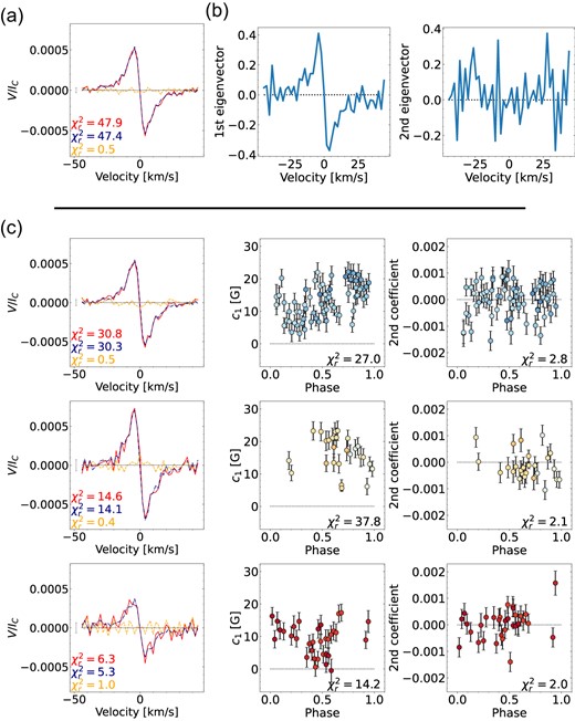
One first determines the mean profile of the whole Stokes V time series, which stores information about the axisymmetric component of the large-scale field. In contrast to Lehmann & Donati (2022), we use the weighted mean profile providing better results for time series such as ours, where all LSD profiles do not have the same SNR. The averaged Stokes V LSD profile can be decomposed into its antisymmetric component (with respect to the line centre), which is related to the poloidal component of the axisymmetric large-scale field, and its symmetric component (with respect to the line centre), which is probing the toroidal component of the axisymmetric large-scale field (see e.g. Fig. 1a).
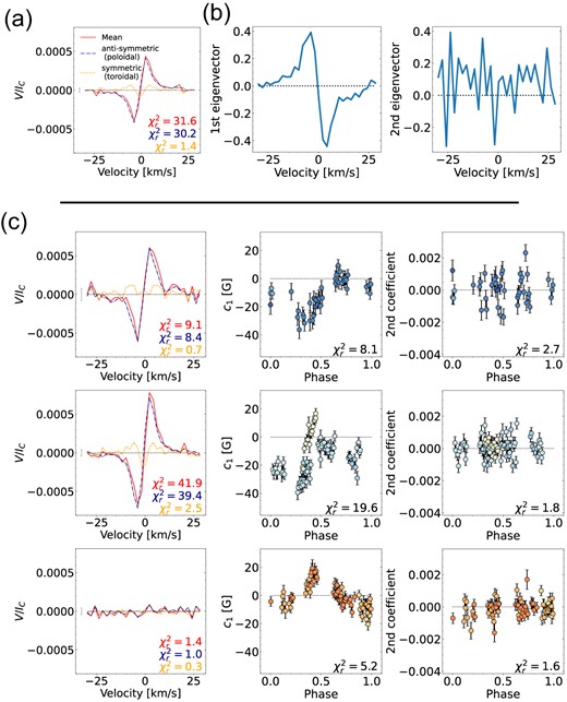
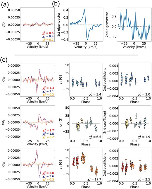
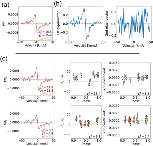
The PCA analysis for Gl 905. a. The mean profile (red) for all observations and its decomposition in the antisymmetric (blue dashed) and symmetric (yellow dotted) components (with respect to the line centre) related to the poloidal and toroidal axisymmetric field, respectively. This mean profile is used to determine the mean-subtracted Stokes V profiles to which we apply PCA, yielding the eigenvectors and coefficients shown in panels b and c. b. The first two eigenvectors of the mean-subtracted Stokes V profiles. c. The mean profile (left column), c1 (the scaled and translated first PCA coefficient introduced in Section 3.2, middle column), and the coefficients of the second eigenvector (right column) for each season (one season per row). The mean profiles of the individual seasons are plotted in the same format as above. The coefficients are colour-coded by rotation cycle.
To evaluate the non-axisymmetric field, we subtract the weighted mean profile (taken over all seasons) from the Stokes V time series removing the signal of axisymmetric field. The resulting mean-subtracted Stokes V profiles store now the information about the non-axisymmetric component of the large-scale field and are analysed using a weighted PCA (Delchambre 2015) returning eigenvectors and coefficients. In the weighted PCA, the Stokes V profiles are weighted by the squares of their SNRs, taking into account the different noise levels. Thus, for the long time series analysed in this paper, with uneven SNR over the seven semesters, the weighted PCA gives better results than a classical PCA where all profiles are treated equally. The PCA coefficients, and in particular their fluctuation with time, can reveal the complexity of the large-scale field and its long-term temporal evolution.
Given the long time range of the SLS data, we further split the Stokes V time series at successive observing seasons into 2–3 seasons per star. To evaluate the evolution of the axisymmetric field from season to season, we determine the weighted mean profiles per season and compare them to one another (see e.g. Fig. 1 c left column). To study the evolution of the non-axisymmetric field, we compare the coefficients of the different seasons (see e.g. Fig. 1 c middle and right column). We caution that the coefficients are derived from the weighted PCA of the mean-subtracted Stokes V time series using the weighted mean profile computed across all seasons (e.g. Fig. 1a) and not the weighted mean profile of each individual season (e.g. Fig. 1 c left column). The usage of the weighted mean Stokes V profiles of each individual season would prevent a direct comparison of the different seasons. For example, it would centre the coefficients for each season, so that we will lose the information if the non-axisymmetric field becomes more or less positive/negative from one season to another, and also the amplitudes of the coefficients are no longer comparable. Further information about the PCA method can be found in Lehmann & Donati (2022).
In addition, Lehmann & Donati (2022) showed that the sensitivity of the PCA method for toroidal fields decreases for low vesin i. As all our stars have |$v_e \sin i \le 0.5\, \mathrm{km\, s^{-1}}$|, we are likely to miss large-scale toroidal fields. We provide a typical 1σ error bar for the axisymmetric toroidal field for each star and each observing season of our sample.
3.2 Gaussian Process modelling of the time series
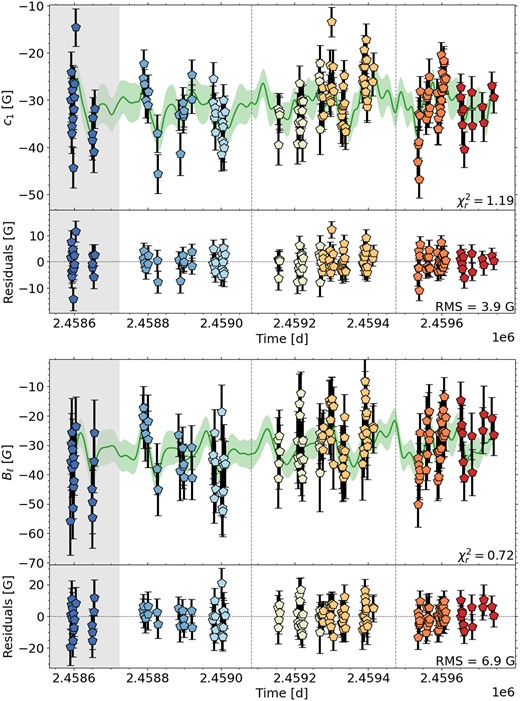
We analyse the temporal evolution of the M dwarf’s topology with the help of the PCA determined coefficients of the mean-substracted Stokes V time series. For our slowly rotating stars, most of the time only the first eigenvector and therefore only the first coefficient shows a signal. To directly compare the temporal evolution of the coefficients with the result from the longitudinal field Bℓ (presented by D23) for the individual stars, we scale and translate the first coefficient, which we call c1, using a linear model (scaling factor and offset), that minimizes the distance between the first coefficients and Bℓ taking into account the measurement errors on Bℓ.
We can re-determine the stellar rotation period Prot of our six M dwarfs using a QP GPR fit to c1 allowing us a direct comparison with the QP GPR results of Bℓ presented by D23.
In contrast to D23, we use the python model presented by Martioli et al. (2022) based on george (Ambikasaran et al. 2015). Our adapted covariance function (or kernel) is given by
where tij = ti − tj is the time difference between the observations i and j, α is the amplitude of the Gaussian Process (GP), l is the decay time describing the typical time-scale on which the modulation pattern evolves, β is the smoothing factor indicating the harmonic complexity of the QP modulation (lower values indicating higher harmonic complexity), and Prot is our new estimate of the stellar rotation period. The GP model parameters are fitted by maximizing the following likelihood function |$\mathcal {L}$| using the python package scipy.optimize:
where K is the QP kernel covariance matrix, Σ is the diagonal variance matrix of c1, S is the diagonal matrix σ2I (with σ an added amount of uncorrelated white noise (Angus et al. 2018) and I the identity matrix), N is the number of observations, and |$\boldsymbol{y}$| corresponds to c1. The posterior distribution of the free parameters is sampled using a Bayesian Markov chain Monte Carlo (MCMC) framework applying the package emcee (Foreman-Mackey et al. 2013). For the MCMC, we use 50 walkers, 200 burn-in samples, and 1000 samples. Table 2 provides a summary of the results for all c1 GPR fits in this study. For three stars, the decay time l was fixed as in D23 (see Table 2). Information about the assumed prior distributions and the posterior distributions for each parameter and each GPR fit can be found in Appendix A.
Summary of the best-fitting parameters of the QP GPR fits applied to c1 for the six M dwarfs in our sample, where rms is the root-mean-square of the residuals and |$\chi ^2_r$| is the reduced chi-square value of the GPR fit. Fixed parameters are shown in italics. A comparison with the results of the GPR fit to the Bℓ data, and with those of D23, is given in Table B1.
| Star | Rotation period | Decay time | Smoothing factor | Amplitude | White noise | rms | |$\chi ^2_{\rm r}$| |
|---|---|---|---|---|---|---|---|
| Prot (d) | l (d) | β | α (G) | σ (G) | (G) | ||
| Gl 905 | |$111.7^{+3.0}_{-3.2}$| | |$133^{+18}_{-22}$| | |$0.50^{+0.09}_{-0.07}$| | |$12.9^{+3.1}_{-2.1}$| | |$0.6^{+0.5}_{-0.4}$| | 3.8 | 0.79 |
| GJ 1289 | |$75.62^{+0.85}_{-0.79}$| | |$129^{+26}_{-24}$| | 0.40 ± 0.05 | |$41.9^{+7.9}_{-6.0}$| | |$1.2^{+1.1}_{-0.8}$| | 6.9 | 0.72 |
| GJ 1151 | |$175.8^{+3.2}_{-3.4}$| | 300 | |$0.40^{+0.10}_{-0.09}$| | |$12.7^{+3.2}_{-2.4}$| | 3.3 ± 0.7 | 5.8 | 0.99 |
| GJ 1286 | |$186.8^{+9.5}_{-5.8}$| | 300 | |$0.23^{+0.05}_{-0.04}$| | |$18.0^{+4.3}_{-3.1}$| | |$2.7^{+1.5}_{-1.7}$| | 7.5 | 1.02 |
| Gl 617B | |$37.8^{+8.5}_{-2.6}$| | |$35^{+8}_{-4}$| | |$0.47^{+0.09}_{-0.05}$| | |$5.9^{+1.2}_{-0.8}$| | |$0.7^{+0.6}_{-0.5}$| | 2.2 | 0.66 |
| Gl 408 | |$175^{+12}_{-14}$| | 200 | |$0.18^{+0.10}_{-0.05}$| | |$4.2^{+0.9}_{-0.8}$| | |$2.2^{+0.5}_{-0.6}$| | 3.8 | 1.19 |
Furthermore, we applied the above GP model to the Bℓ values of D23 (see appendix B). This allows a direct comparison of the GP results for the same Bℓ data set with our GP routine and the GP routine used by D23, as well as a comparison of the GP results for c1 and Bℓ obtained by the same GP routine. In general, we find that c1 has lower rms, often shows lower σ values, and provides smaller errors for Prot when the topology is not highly axisymmetric.
3.3 Zeeman–Doppler imaging
We determined the large-scale vector magnetic field at the surface of the six M dwarfs, for each season, using ZDI. ZDI iteratively builds up the large-scale magnetic field and compares the synthetic Stokes profiles corresponding to the current magnetic map, assuming solid body rotation, with the observed Stokes profiles until it converges on the requested reduced chi-square value |$\chi ^2_r$| between the observed and synthetic data. The problem being ill-posed, i.e. with an infinite number of solutions featuring the requested agreement to the data, ZDI chooses the one with maximum entropy, (i.e. minimum information in our case, Skilling & Bryan 1984). The surface magnetic field is described with a spherical harmonics expansion given in Donati et al. (2006), where the αℓ, m and βℓ, m coefficients of the poloidal component are modified as indicated in Lehmann & Donati (2022, equation B1). To compute synthetic Stokes profiles, the stellar surface is decomposed into a grid of 1000 cells. For each cell, the local Stokes V and I profiles are determined using Unno–Rachkovsky’s analytical solution to the equations of the polarized radiative transfer in a plane-parallel Milne–Eddington atmosphere (Landi Degl’Innocenti & Landolfi 2004). The Stokes profiles are integrated over the visible hemisphere for each observing phase applying a mean wavelength of 1700 nm and a Landé factor of 1.2.
For the slowly rotating M dwarfs of our sample, we see no obvious variations in the Stokes I LSD profiles beyond those attributable to radial velocity variations, so that we only use the Stokes V profiles for determining the magnetic field map via ZDI. Nevertheless, we make sure that the synthetic Stokes I profiles computed with ZDI agree well with the averaged observed Stokes I profile, especially in terms of width and depth. We assumed a fraction fV of each grid cell, which actually contributes to the Stokes V profile. This fraction fV is called filling factor of the large-scale field and is set equally to all cells, see also Morin et al. (2010) and Kochukhov (2021). For each star, we set fV = 0.1 motivated by the results of Klein et al. (2021) for the slow rotator Proxima Centauri and the results of Moutou et al. (2017) for the SPIRou sample. We confirm the choice of fV = 0.1 by finding lower |$\chi ^2_r$| values with fV = 0.1 compared to fV = 1 for each season of the different M dwarfs. The filling factor for the Stokes I profiles is set to fI = 1.0 in consistency with the literature (Morin et al. 2010; Kochukhov 2021). The vesin i of our sample is |$\le 0.5\, \mathrm{km\, s^{-1}}$| (see Table 1) and prevents us from reliably determining the inclination of the stellar rotation axis for the M dwarfs, so that we set the inclination to 60° for all M dwarfs. This is motivated by the steep modulation patterns seen for Bℓ and c1 for most targets that cannot be obtained for pole-on viewed stars. Another reason is that higher values of i are intrinsically more likely than smaller ones. We restrict the spherical harmonics of the ZDI reconstructions to ℓ = 7, as we see little magnetic energy stored in ℓ ∼ 5–7.
4 Gl 905
The first star in our sample is the M5.5V dwarf Gl 905 (HH And, Ross 248) with a mass of |$0.15\pm 0.02\,$| M⊙, (Cristofari et al. 2022). For our analysis, we use 219 Stokes IV LSD profiles observed with SPIRou between 2019 April and 2022 June and split the data in three seasons (2019 April–December, 2020 May–2021 January, and 2021 June–2022 January) for the per-season analysis. The 15 profiles collected in 2022 June at the beginning of a new season, only covering 9 per cent of a rotation cycle, were left out of the per-season analysis.
4.1 PCA analysis of Gl 905
First, we investigate the large-scale field topology using PCA (Lehmann & Donati 2022). The weighted mean profile of all Stokes V profiles is antisymmetric with respect to the line centre indicating a poloidal axisymmetric large-scale field (see Fig. 1a). The symmetric component of Gl 905’s mean profile exceeds the noise level (|$\chi ^2_r = 1.4$|) but is likely due to an uneven phase coverage in the season 2020/21 (see Section 4.2). In Fig. 1(b), we show the first two eigenvectors of the mean-subtracted Stokes V profiles allowing the analysis of the non-axisymmetric field. Only the first eigenvector shows an antisymmetric signal with respect to the line centre. All other eigenvectors display noise.
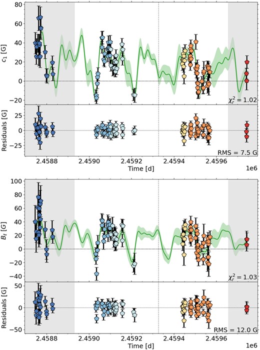
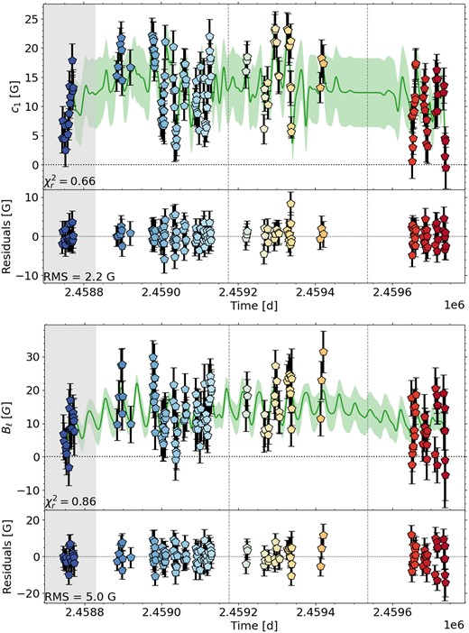
In Fig. 2 top, we plot the temporal evolution of c1, which appears very similar to the temporal evolution of Bℓ determined with our GP model (see Fig. 2 bottom) and to D23’s results (see fig. A12 middle in D23). When only one eigenvector is significant, as it is the case here for Gl 905, the c1 curve mimics that of Bℓ (Lehmann & Donati 2022).
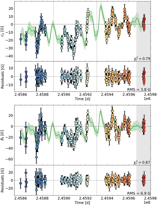
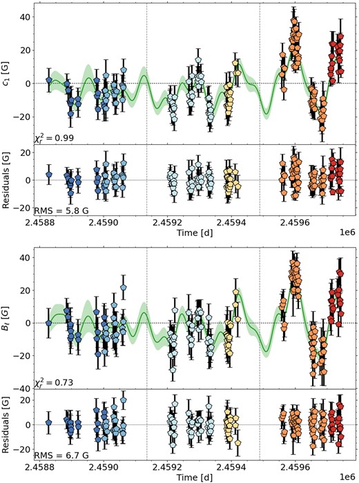
Temporal variations of c1 (top) and longitudinal field Bℓ (bottom) for Gl 905. We show the QP GPR fit and its 1σ area as green shaded region in the top panel and the residuals in the bottom panel for both variables. The plot symbols are colour-coded by rotation cycle. The vertical grey lines separate the analysed seasons. The grey shaded region indicates a season for which not enough data were available for a reliable PCA and ZDI analysis.
Our QP GPR model of c1 finds a rotation period of |$P_{\mathrm{rot}}= 111.7^{+3.0}_{-3.2}\, \mathrm{d}$| and decay time of |$l = 133^{+18}_{-22}\, \mathrm{d}$| very similar to the values derived by D23 (|$P_{\mathrm{rot}}= 114.3\pm 2.8\, \mathrm{d}$| and |$l = 129^{+25}_{-21}\, \mathrm{d}$|) and Fouqué et al. (2023) (|$P_{\mathrm{rot}}= 109.5^{+4.9}_{-5.4}\, \mathrm{d}$| and |$l = 149^{+26}_{-25}\, \mathrm{d}$|) and also consistent with our GP fit of D23’s Bℓ values (|$P_{\mathrm{rot}}= 114.4^{+3.5}_{-2.4}\, \mathrm{d}$| and |$l = 130^{+25}_{-32}\, \mathrm{d}$|), see Tables 2 and B1. For consistency, we use the rotation periods found by D23 to determine the rotation phase (see Table A1) and to model the ZDI maps for all six stars in our sample (see Table 1).
In Fig. 1(c), we plot the mean profiles (left column) and the phase-folded coefficient curves colour-coded by rotation phase (middle and right columns) for the three seasons (one season per row). They exhibit large changes in the large-scale field topology from season to season, allowing us to draw first conclusions about the field evolution of Gl 905. We recall that the coefficients for all three seasons are computed from the mean-subtracted Stokes V profiles, using the weighted mean derived from the full data set, and not from the profiles of each season. The same applies to the five M dwarfs discussed in Sections 5–9.
The mean profiles of the first two seasons (2019 and 2020/21) are antisymmetric with respect to the line centre and indicate a mostly poloidal axisymmetric field although the symmetric component is larger for 2020/21 (see Fig. 1c). This may reflect an increasing toroidal field but is more likely due to the uneven phase coverage of this season (with more than 75 per cent of the observations concentrating between phase 0.3 and 0.75).
For the first season 2019, c1 features a roughly sinusoidal behaviour indicating a mainly dipolar configuration. For 2020/21, c1 appears more complex than for 2019 implying that the field becomes more complex, too. For the last season 2021/22, the topology changes more drastically: the mean profile is close to zero indicating a much lower axisymmetric component than before. The phase at which c1 reaches its maximum is shifted, with c1 being more positive now, while it is mainly negative before. Considering the sign of the mean profile and the eigenvector, this suggest that the main polarity of the large-scale field is evolving from a predominantly negative polarity to a positive polarity. We can conclude from the PCA analysis that the large-scale field topology becomes more complex from 2019 to 2020/21 before it becomes mostly non-axisymmetric and possibly initiates a polarity reversal.
4.2 ZDI reconstructions of Gl 905
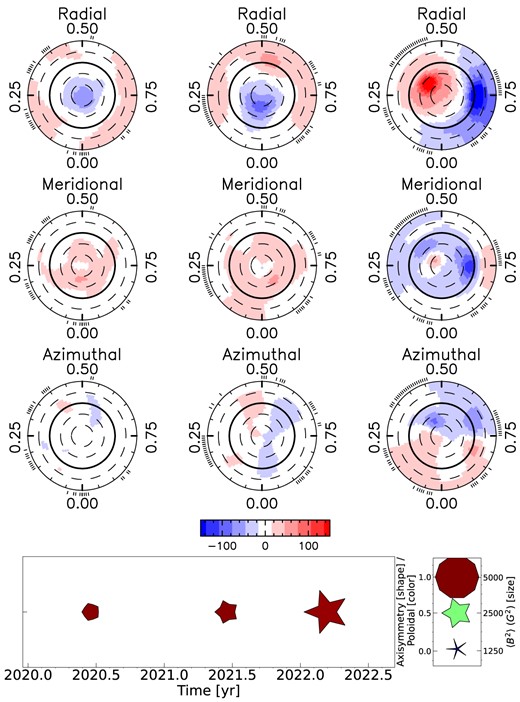
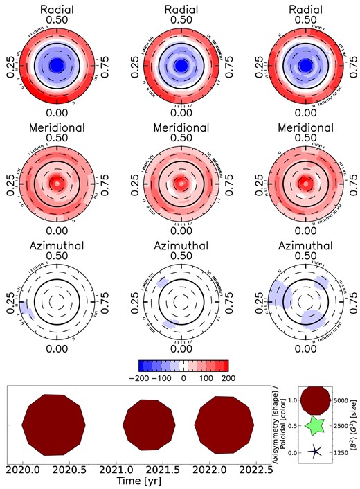
We conclude our analysis by deriving vector magnetic field maps for Gl 905 using ZDI, for each of the three main observing seasons. The maps are shown in Fig. 3 and their magnetic properties are summarized in Table 3. We were able to fit all three ZDI maps down to |$\chi _r^2 \approx 1.0$| assuming |$P_{\mathrm{rot}} = 114.3\, \mathrm{d}$|, |$v_e \sin i = 0.06\, \mathrm{km\, s^{-1}}$|, i = 60°, and fV = 0.1.
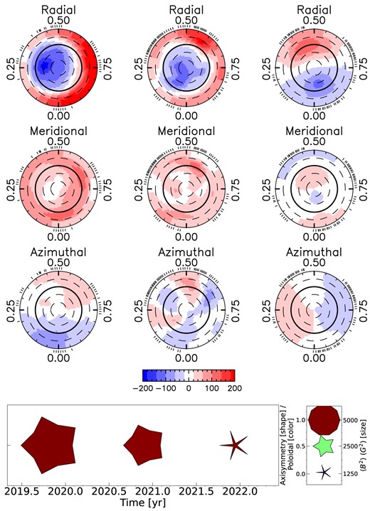
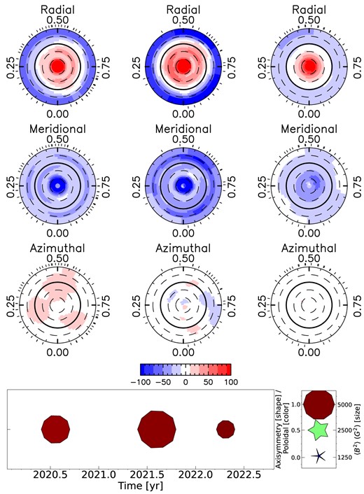
The magnetic field maps of Gl 905 shown in a flattened polar view for the radial (top row), meridional (middle row), and azimuthal component (bottom row). In each plot, the visible north pole is in the centre, the thick line depicts the equator, and the dashed line the latitudes in 30° step. The ticks outside the plot illustrate the observing phases. The different seasons are shown next to each other (one season per column). The colour bar below the third row is used for all maps and indicates the magnetic field strength in G. The bottom panel summarizes the main characteristics of the large-scale field of Gl 905 and its evolution with time. For each season, the symbol size indicates the magnetic energy, the symbol shape the fractional energy in the axisymmetric component, and the symbol colour the fractional energy stored into the poloidal component of the field (see legend to the right).
Magnetic properties of Gl 905 extracted from the ZDI maps per season: the start and end month of the observations used for the ZDI maps, the surface averaged unsigned magnetic field 〈BV〉[G], the surface average unsigned dipole magnetic field 〈Bdip〉[G], the typical 1σ error bar on the ZDI reconstructed surface averaged toroidal field |$\sigma _{\langle B_\mathrm{tor} \rangle }$|, the fractional energy of the poloidal field, the fractional energy of the axisymmetric field (only m = 0 modes), the fractional energy of the dipole component, the tilt angle of the dipole (ℓ = 1) with respect to the negative pole, the phase at which the dipole field faces the observer, the reduced χ2 values for the Stokes V profiles (|$\chi ^2_{r,V}$|; corresponding to a |${\bf B} = 0\,$| G fit), for the ZDI fit of the Stokes V profiles (|$\chi ^2_{r,V,\mathrm{ZDI}}$|) and for the Null profiles (|$\chi ^2_{r,N}$|), and the number of observations per season (nb. obs).
| Season | 2019 | 2020/21 | 2021/22 |
|---|---|---|---|
| Start | 2019 Apr | 2020 May | 2021 June |
| End | 2019 Dec | 2021 Jan | 2022 Jan |
| 〈BV〉 (G) | 128 | 89 | 64 |
| 〈Bdip〉 (G) | 124 | 80 | 64 |
| |$\sigma _{\langle B_\mathrm{tor} \rangle }$| (G) | 179 | 55 | 84 |
| fpol | 1.0 | 0.99 | 1.0 |
| faxi | 0.68 | 0.7 | 0.04 |
| fdip | 0.93 | 0.79 | 0.94 |
| Dipole tilt angle | 33° | 22° | 83° |
| Pointing phase | 0.29 | 0.12 | 0.96 |
| |$\chi ^2_{r,V}$| | 1.94 | 3.81 | 1.47 |
| |$\chi ^2_{r,V,\mathrm{ZDI}}$| | 1.04 | 1.12 | 1.02 |
| |$\chi ^2_{r,N}$| | 1.22 | 1.10 | 1.04 |
| Nb. obs | 43 | 84 | 77 |
The ZDI maps confirm the conclusions we derived from the PCA analysis. The topology gets indeed more complex from 2019 to 2020/21 and the degree of axisymmetry decreases from around 70 per cent to 4 per cent for the last season 2021/22. The surface mean magnetic field decreases from |$128$| to |$64\, \mathrm{G}$|. Most prominent is the hint of an ongoing polarity reversal from negative to positive radial field taking place in the last season.
To test whether the symmetric component of the mean profile for season 2020/21 indeed results from an uneven phase coverage, we simulate 24 evenly phased Stokes V LSD profiles from the 2020/21 ZDI map (see Fig. 3 middle column) and determine the corresponding mean profile and its symmetric and antisymmetric components (see Fig. C1). The symmetric component disappears with even phase sampling, confirming that the mean LSD profile provides no observational hint for a large-scale axisymmetric toroidal field at the surface of Gl 905.
The reconstructed surface averaged toroidal field 〈Btor〉 is lower than 10 G for each season. To derive a 1σ error bar on the simplest possible large-scale axisymmetric toroidal field (described with spherical harmonics coefficients ℓ = 1 and m = 0) at the stellar surface, we proceed in the following way: (1) artificially add an axisymmetric toroidal field of strength 〈Btor〉 to the reconstructed ZDI map, (2) simulate the corresponding Stokes V LSD profiles with the phase coverage and SNR of the actual observations, and (3) compute the new χ2 with respect to the observed LSD profiles and raise 〈Btor〉 until χ2 is increased by 1 with respect to the optimal ZDI fit. We find 1σ error bars ranging from 180 G in 2019 down to 55 G in 2020/21.
5 GJ 1289
The fully convective M dwarf GJ 1289 (|$M = 0.21\pm 0.02\,$| M⊙, Cristofari et al. 2022) is the next star in our sample. SPIRou observed GJ 1289 from 2019 September until 2022 June providing a time series of 204 LSD profiles split into three seasons (2019 June–December, 2020 May–2021 January, and 2021 June–2022 January) for the per-season analysis. As for Gl 905, the 14 profiles collected in 2022 June at the beginning of a new season, only covering 16 per cent of a rotation cycle, were left out of the per-season analysis.
5.1 PCA analysis of GJ 1289
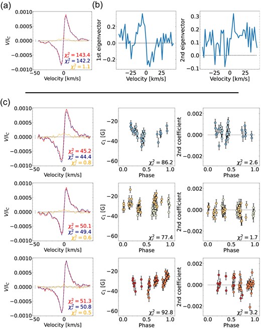
The mean profile is perfectly antisymmetric with respect to the line centre indicating a dominant axisymmetric poloidal component (see Fig. 4a). Both the first and second eigenvectors are found to be antisymmetric with respect to the line centre, which is a strong hint of a non-axisymmetric poloidal component (see Fig. 4b). All further eigenvectors trace noise.
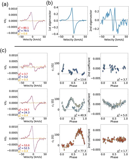
Same as Fig. 1 for GJ 1289.
The QP GPR fit applied to c1 (see Fig. 5 top) finds |$P_{\mathrm{rot}}= 75.62^{+0.85}_{-0.79}\, \mathrm{d}$| with a decay time of |$l = 129^{+26}_{-24}\, \mathrm{d}$| fitting all five parameters with a |$\chi ^2_r = 0.72$| (see Table 2). The rotation period and decay time agree with the values found from the GPR fits of Bℓ found by D23 (|$P_{\mathrm{rot}}= 73.66\pm 0.92\, \mathrm{d}$| and |$l = 152^{+32}_{-27}\, \mathrm{d}$|) and Fouqué et al. (2023) (|$P_{\mathrm{rot}}= 74.0^{+1.5}_{-1.3}\, \mathrm{d}$| and |$l = 142^{+33}_{-26}\, \mathrm{d}$|) and are also consistent with our GP fit of the Bℓ values of D23 (|$P_{\mathrm{rot}}= 73.67^{+1.01}_{-0.91}\, \mathrm{d}$| and |$l = 152^{+30}_{-28}\, \mathrm{d}$|, see Fig. 5 bottom).
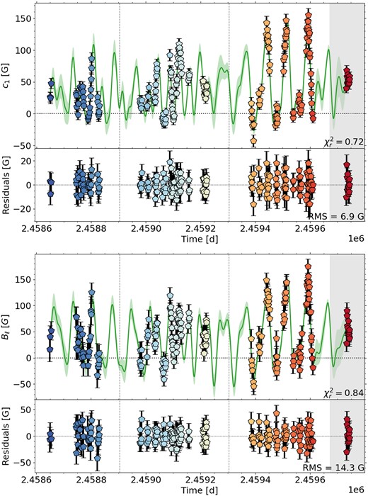
Same as Fig. 2 for GJ 1289.
In Fig. 4(c), we show the mean profile and the phase-folded coefficients split by season. Comparing the mean profiles of the three seasons, the axisymmetric component grows in amplitude and stays always poloidal. As the amplitude of the coefficients increases as well, the magnetic field becomes in general stronger.
The phase-folded coefficient curves indicate a rapidly evolving and complex large-scale field, as we see variations from one rotation cycle to the next (see season 2020/21) and trends that are more complex than sine waves (e.g. for 2019 and 2020/21). Furthermore, season 2020/21 stands out, with the second eigenvector contributing significantly to the Stokes V signal before disappearing again for the last season 2021/22, for which c1 shows a simpler trend.
5.2 ZDI reconstructions of GJ 1289
We were able to fit the Stokes V profiles for all seasons down to |$\chi ^2_r \approx 1.0$| assuming |$P_{\mathrm{rot}}= 73.66\, \mathrm{d},\ v_e \sin i = 0.14\, \mathrm{km\, s^{-1}},\ i = 60^\circ ,\mathrm{ and}\ f_V = 0.1$|. In the first season, the data set only includes about half of the observations of those from the two other seasons and the achieved |$\chi ^2_{r,V} = 1.46$| is several times lower than the |$\chi ^2_{r,V}$| of the following seasons (see Table 4). In the first season, ZDI reveals a weak marginally complex field topology. In 2020/21, the surface averaged field 〈BV〉 becomes twice as large due to a growing axisymmetric poloidal dipole and ZDI reconstructs a more complex azimuthal field, featuring a quadrupolar non-axisymmetric azimuthal structure (see Fig. 6). In the last season 2021/22, the dipole tilts more strongly to 39° and dominates the field topology (see Table 4). The toroidal field of the ZDI maps varies between 7 and 25 G, which is again lower than the typical 1σ error bar that we derive ranging from 40 to 100 G.
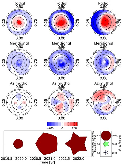
Same as Fig. 3 for GJ 1289.
Same as Table 3 for GJ 1289. The tilt angle now refers to the positive pole.
| Season | 2019 | 2020/21 | 2021/22 |
|---|---|---|---|
| Start | 2019 June | 2020 May | 2021 June |
| End | 2019 Dec | 2021 Jan | 2022 Jan |
| 〈BV〉 (G) | 83 | 199 | 214 |
| 〈Bdip〉 (G) | 79 | 194 | 200 |
| |$\sigma _{\langle B_\mathrm{tor} \rangle }$| (G) | 42 | 57 | 100 |
| fpol | 0.99 | 0.98 | 0.99 |
| faxi | 0.93 | 0.86 | 0.57 |
| fdip | 0.67 | 0.79 | 0.82 |
| Dipole tilt angle | 11° | 8° | 39° |
| Pointing phase | 0.19 | 0.18 | 0.74 |
| |$\chi ^2_{r,V}$| | 1.46 | 3.60 | 8.34 |
| |$\chi ^2_{r,V,\mathrm{ZDI}}$| | 0.98 | 1.04 | 0.98 |
| |$\chi ^2_{r,N}$| | 0.95 | 0.94 | 0.97 |
| Nb. obs | 35 | 80 | 75 |
6 GJ 1151
Our next star, GJ 1151, is also a fully convective M dwarf (|$M = 0.17\pm 0.02\,$| M⊙, Cristofari et al. 2022) and was observed between 2019 December and 2022 June with SPIRou providing us 158 LSD profiles (seasons: 2019 December–2020 July, 2020 December–2021 July, 2021 December–2022 June).
6.1 PCA analysis of GJ 1151
The mean profile is close to zero indicating a strongly non-axisymmetric topology (see Fig. 7a). Only the first eigenvector of the mean-subtracted Stokes V profiles significantly differs from the noise and features an antisymmetric signal with respect to the line centre (see Fig. 7b).
Same as Fig. 1 for GJ 1151.
The QP GPR model fits c1 down to a |$\chi ^2_r = 0.99$| (see Fig. 8 top). We fix the decay time to 300 d similar to D23 and find a |$P_{\mathrm{rot}}= 175.8^{+3.2}_{-3.4}\, \mathrm{d}$| similar to the results of D23 (|$P_{\mathrm{rot}}= 175.6\pm 4.9\, \mathrm{d}$|) and our own GP fit of Bℓ (|$P_{\mathrm{rot}}= 176.1^{+3.6}_{-4.1}\, \mathrm{d}$|), see also Fig. 8 bottom. Our rotation period is a bit higher than the one found by Fouqué et al. (2023) (|$P_{\mathrm{rot}}= 158\pm 12\, \mathrm{d}$|) but compatible at 1σ.
Same as Fig. 2 for GJ 1151.
The mean profile of the first two seasons is antisymmetric with respect to the line centre (axisymmetric poloidal field) and is relatively weak (see Fig. 7c). The coefficient c1 shows no obvious trend with phase for the first season 2019/20 and just start to display a weak variation with phase for 2020/21. The low amplitude of the mean profiles and coefficients indicate that the magnetic field must be very weak during the first two seasons. For the last season 2021/22, the amplitude of the mean profile is twice as high as before and also c1 shows a higher amplitude (|$\chi ^2_r = 7.9$|), indicating that the magnetic field increases significantly for 2021/22. We also notice that the sign of the mean profile (and therefore the projected main polarity of the large-scale magnetic field) changed from negative to positive for the last season, hence why the mean profile over the whole time series is close to zero (see Fig. 7a).
6.2 ZDI reconstructions of GJ 1151
We could fit the Stokes V profiles down to |$\chi ^2_r \approx 1.0$| assuming |$P_{\mathrm{rot}}= 175.6\, \mathrm{d}$|, |$f_V = 0.1, v_e \sin i = 0.05\, \mathrm{km\, s^{-1}}$|, and inclination of i = 60°.
For the first two seasons, the Stokes V profiles are weak (see Fig. C6) and so is the reconstructed field (see Fig. 9), with a dominant negative polarity in the upper hemisphere that is consistent with the corresponding mean profiles. We see a small increase of 〈BV〉 in the second season of 2020/21 explaining the higher amplitude of c1 seen in the PCA analysis (see Fig. 7c). For the last season 2021/22, the ZDI map shows a strongly tilted dipole (tilt angle = 55°), that flipped polarity, and the surface averaged field is more than twice as high as before (〈BV〉 = 63 G). To the best of our knowledge this is the first polarity reversal seen in the vector magnetic field map of an M dwarf.
The reconstructed toroidal field 〈Btor〉 is lower than 8 G for all seasons of GJ 1151 and we find that the 1σ error bar on the toroidal field ranges between 370 and 450 G (see Table 5).
7 GJ 1286
GJ 1286 (LHS 546) is the lowest mass M dwarf in our sample (|$M = 0.12\pm 0.02\,$| M⊙, Cristofari et al. 2022). We analyse here 104 observations, which we split into two seasons (2020 June–December and 2021 August–December) for the per-season analysis. As the first and last season (2019 September–December and 2022 June) do not contain enough observations, we once more left 21 LSD profiles out of the per-season analysis.
7.1 PCA analysis of GJ 1286
The mean profile of GJ 1286 is antisymmetric with respect to the line centre and appears more noisy than usual but clearly indicates a purely axisymmetric poloidal field (see Fig. 10a). The first eigenvector has an antisymmetric shape, too, and is the only one that emerges from the noise (see Fig. 10b).
Same as Fig. 3 for GJ 1151. Note that the magnetic field switches polarity.
Same as Fig. 1 for GJ 1286.
The best-fitting model of the QP GPR for c1 finds a |$P_{\mathrm{rot}}= 186.8^{+9.5}_{-5.8}\, \mathrm{d}$| for a fixed decay time of 300 d reaching a |$\chi ^2_r = 1.02$| similar to the GPR fit of Bℓ (see Fig. 11). The rotation period agrees with the values found by D23 and Fouqué et al. (2023) (|$P_{\mathrm{rot}}= 178\pm 15\, \mathrm{d}$| and |$P_{\mathrm{rot}}= 203^{+14}_{-21}\, \mathrm{d}$|, respectively) and our own GP result for Bℓ (|$P_{\mathrm{rot}}= 181^{+18}_{-13}\, \mathrm{d}$|).
Same as Fig. 2 for GJ 1286.
The mean profile of season 2020 is nearly twice as high as for 2021 (see Fig. 10c). Also c1 shows a lower amplitude for 2021. We can therefore conclude that the surface averaged field decreases for 2021. The field topology becomes simpler as the c1 curve gets less complex with phase for 2021.
7.2 ZDI reconstructions of GJ 1286
We fitted the LSD Stokes V profiles of the two seasons for GJ 1286 down to |$\chi ^2_r \approx 1.0$|, assuming |$P_{\mathrm{rot}}= 178\, \mathrm{d}$|, |$f_V = 0.1, v_e \sin i = 0.03\, \mathrm{km\, s^{-1}}$|, and i = 60°.
As concluded from the PCA analysis, the ZDI maps confirm that the topology becomes simpler and weaker: the fractional energy of the dipole component fdip increases from 0.73 to 0.79, while 〈BV〉 decreases by almost half from |$113\,$| to |$71\,$| G (see Fig. 12 and Table 6). The reconstructed toroidal field 〈Btor〉 of the seasons are 9 and 6 G, respectively, while the typical 1σ error bars on the axisymmetric toroidal field are 325 and 300 G, respectively.
Same as Fig. 3 for GJ 1286.
Same as Table 3 for GJ 1151.
| Season | 2019/20 | 2020/21 | 2021/22 |
|---|---|---|---|
| Start | 2019 Dec | 2020 Dec | 2021 Dec |
| End | 2020 July | 2021 July | 2022 June |
| 〈BV〉 (G) | 26 | 35 | 63 |
| 〈Bdip〉 (G) | 23 | 32 | 62 |
| |$\sigma _{\langle B_\mathrm{tor} \rangle }$| (G) | 448 | 378 | 372 |
| fpol | 0.99 | 0.99 | 0.98 |
| faxi | 0.84 | 0.64 | 0.38 |
| fdip | 0.64 | 0.72 | 0.75 |
| Dipole tilt angle | 4° | 32° | −55° |
| Pointing phase | 0.44 | 0.05 | 0.33 |
| |$\chi ^2_{r,V}$| | 1.16 | 1.25 | 2.57 |
| |$\chi ^2_{r,V,\mathrm{ZDI}}$| | 1.00 | 0.87 | 0.91 |
| |$\chi ^2_{r,N}$| | 1.00 | 1.01 | 0.88 |
| Nb. obs | 38 | 53 | 67 |
Same as Table 4 for GJ 1286.
| Season | 2020 | 2021 |
|---|---|---|
| Start | 2020 June | 2021 Aug |
| End | 2020 Dec | 2021 Dec |
| 〈BV〉 (G) | 113 | 71 |
| 〈Bdip〉 (G) | 103 | 67 |
| |$\sigma _{\langle B_\mathrm{tor} \rangle }$| (G) | 325 | 300 |
| fpol | 0.99 | 0.99 |
| faxi | 0.67 | 0.79 |
| fdip | 0.73 | 0.79 |
| Dipole tilt angle | 28° | 25° |
| Pointing phase | 0.03 | 0.95 |
| |$\chi ^2_{r,V}$| | 2.21 | 1.65 |
| |$\chi ^2_{r,V,\mathrm{ZDI}}$| | 0.87 | 0.94 |
| |$\chi ^2_{r,N}$| | 1.05 | 0.82 |
| Nb. obs | 38 | 45 |
8 Gl 617B
Gl 617B (EW Dra, HIP 79762, LHS 3176) is a partly convective M dwarf with |$M = 0.45\pm 0.02\,$| M⊙ (Cristofari et al. 2022) and was observed between 2019 September and 2022 June with SPIRou. Our following analysis is based on 144 LSD Stokes spectra, which we split into three seasons (2020 February–October, 2021 January–July, and 2022 March–June) for the per-season analysis. As for the other stars, the first 15 spectra collected in 2019 were left out of the per-season analysis.
8.1 PCA analysis of Gl 617B
We find that the mean profile is much larger than the mean-subtracted Stokes V profiles indicating that the axisymmetric component of the magnetic field is dominant (see Fig. 13a). The mean profile is again antisymmetric with respect to the line centre, indicating an axisymmetric poloidal field. The first eigenvector is already very noisy and is the only one that shows a clear signal, confirming that the field is indeed dominantly axisymmetric (see Fig. 13b).
Same as Fig. 1 for Gl 617B.
The QP GPR model fits c1 down to a |$\chi ^2_r = 0.66$| finding a rotation period of |$37.8^{+8.5}_{-2.6}\, \mathrm{d}$| in agreement with the results of D23 (|$P_{\mathrm{rot}}= 40.4\pm 3.0\, \mathrm{d}$|) and our GP fit of Bℓ (|$P_{\mathrm{rot}}= 40.6^{+2.1}_{-4.4}\, \mathrm{d}$|, see Fig. 14). However, the decay time for the GP fit of c1 with |$l = 35^{+8}_{-4}\, \mathrm{d}$| is shorter than the results determined from the Bℓ curves (|$l = 69^{+35}_{-23}\, \mathrm{d}$| for D23 and |$l = 82^{+45}_{-30}\, \mathrm{d}$| from our own fit of Bℓ). Fouqué et al. (2023) found no clear periodic variation using the apero pipeline reduced spectra of Gl 617B.
Same as Fig. 2 for Gl 617B.
The mean profile is antisymmetric to the line centre and therefore poloidal dominated for all three seasons, but varies in amplitude (see Fig. 13c, left column). None the less, c1 traces a varying non-axisymmetric component. Season 2020 shows the highest range in amplitude of c1, indicating the largest dipole tilt angle of all three seasons, although it will still be small (<20°) due to the predominantly axisymmetric topology of Gl 617B.
8.2 ZDI reconstructions of Gl 617B
We could fit Gl 617B down to |$\chi ^2_r \approx 1.0$| assuming |$P_{\mathrm{rot}}= 40.4\, \mathrm{d}, f_V = 0.1, v_e\sin i = 0.50\, \mathrm{km\, s^{-1}}, \mathrm{ and}\, i = 60^\circ$|. The ZDI maps confirm a very axisymmetric, poloidal configuration (see Fig. 15). The axisymmetry is always equal to or greater than 97 per cent, so variations of the non-axisymmetric field are difficult to see, but appear largest in 2021 (see Table 7). The data set in season 2020 shows the largest tilt angle (7°) as predicted by the PCA analysis. The reconstructed toroidal field 〈Btor〉 reaches 9 G for 2020, 6 G for 2021, and 2 G for 2022, while the estimated 1σ error bar on the axisymmetric toroidal field is about 7 G in 2020, 13 G in 2021, and 6 G in 2022, which is a lower uncertainty than for the other M dwarfs thanks to the higher |$v_e \sin i = 0.5\, \mathrm{km\, s^{-1}}$| of Gl 617B.
Same as Fig. 3 for Gl 617B.
Same as Table 4 for Gl 617B.
| Season | 2020 | 2021 | 2022 |
|---|---|---|---|
| Start | 2020 Feb | 2021 Jan | 2022 Mar |
| End | 2020 Oct | 2021 July | 2022 June |
| 〈BV〉 (G) | 53 | 75 | 36 |
| 〈Bdip〉 (G) | 52 | 73 | 35 |
| |$\sigma _{\langle B_\mathrm{tor} \rangle }$| (G) | 7 | 13 | 6 |
| fpol | 0.98 | 0.99 | 1.0 |
| faxi | 0.98 | 0.97 | 0.98 |
| fdip | 0.67 | 0.74 | 0.71 |
| Dipole tilt angle | 7° | 4° | 3° |
| Pointing phase | 0.74 | 0.47 | 0.87 |
| |$\chi ^2_{r,V}$| | 2.37 | 3.08 | 1.59 |
| |$\chi ^2_{r,V,\mathrm{ZDI}}$| | 0.99 | 0.95 | 1.00 |
| |$\chi ^2_{r,N}$| | 1.00 | 1.06 | 0.89 |
| Nb. obs | 70 | 26 | 33 |
We see 〈BV〉 changing by approximately ±25 G for the three seasons, otherwise the main properties of the maps are similar (see Table 7).
For highly axisymmetric topologies, it is difficult to infer the inclination i. It may be that i is actually lower for Gl 617B. We provide the ZDI maps for an inclination i = 30° and |$v_e \sin i = 0.29\, \mathrm{km\, s^{-1}}$|, while otherwise using the same parameters (see Fig. C2). The |$\chi ^2_r$| values reached for the ZDI fits are slightly higher for i = 30° than for i = 60°.
9 Gl 408
Gl 408 (Ross 104, HIP 53767, LHS 6193) is another partly convective star, with |$M = 0.38\pm 0.02\,$| M⊙, (Cristofari et al. 2022). SPIRou observed Gl 408 between 2019 April and 2022 June. We use 157 Stokes V profiles for the following analysis split into three seasons (2019 October–2020 June, 2020 October–2021 July, and 2021 November–2022 June) for the per-season analysis. As for the other stars, the first 17 spectra collected in early 2019 were left out of the per-season analysis.
9.1 PCA analysis of Gl 408
Gl 408 has the strongest mean profile compared to the mean-subtracted profile in our sample (see Figs 16 a and C9). The first eigenvector of Gl 408 (the only one showing a signal) is already noisy, a strong indication of a very axisymmetric field topology (see Fig. 16b).
Fig. 17 (top) presents the QP GPR fit of c1, which gives a |$P_{\mathrm{rot}}= 175^{+12}_{-14}\, \mathrm{d}$| similar to D23 determining |$P_{\mathrm{rot}}= 171.0\pm 8.4\, \mathrm{d}$|. Fitting Bℓ with our GP routines, we derive a |$P_{\mathrm{rot}}= 170.7^{+7.1}_{-9.8}\, \mathrm{d}$| (see Fig. 17 bottom). The decay time was fixed at 200 d for both variables following D23. However, we find a decay time of |$\approx 200\pm 70\, \mathrm{d}$| but higher χ2 for GPR fits without fixing the decay time. The apero reduced spectra of Gl 408 did not allow Fouqué et al. (2023) to determine a rotation period.
Same as Fig. 1 for Gl 408.
Same as Fig. 2 for Gl 408.
In Fig. 16(c), we see that c1 is mostly flat for all three seasons, again indicating a highly axisymmetric topology. All mean profiles are antisymmetric with respect to the line centre and show an axisymmetric poloidal large-scale field.
9.2 ZDI reconstructions of Gl 408
All three seasons could be fitted down to χ2 ≈ 1.0 assuming |$P_{\mathrm{rot}}= 171.0\, \mathrm{d}, f_V = 0.1, v_e \sin i = 0.10\, \mathrm{km\, s^{-1}}, \,\mathrm{ and}\,i = 60^\circ$|. The topology changes little over the three seasons and is characterized by a strong, axisymmetric, poloidal dipole of negative polarity (see Fig. 18). It is the most stable topology in our sample and only 〈BV〉 varies marginally between 106 and 130 G (see Table 8). We find a 1σ error bar on the axisymmetric toroidal field of 55–81 G for Gl 408 whereas the reconstructed 〈Btor〉 ranges between |$4\,\mathrm{ and}\,13\,$| G.
Same as Fig. 3 for Gl 408.
Same as Table 3 for Gl 408.
| Season | 2019/20 | 2020/21 | 2021/22 |
|---|---|---|---|
| Start | 2019 Oct | 2020 Oct | 2021 Nov |
| End | 2020 June | 2021 July | 2022 June |
| 〈BV〉 | 130 | 106 | 120 |
| 〈Bdip〉 (G) | 129 | 104 | 117 |
| |$\sigma _{\langle B_\mathrm{tor} \rangle }$| (G) | 81 | 55 | 57 |
| fpol | 1.0 | 1.0 | 0.99 |
| faxi | 0.98 | 0.98 | 0.98 |
| fdip | 0.82 | 0.77 | 0.78 |
| Dipole tilt angle | 6° | 4° | 4° |
| Pointing phase | 0.53 | 0.44 | 0.47 |
| |$\chi ^2_{r,V}$| | 5.63 | 4.13 | 5.66 |
| |$\chi ^2_{r,V,\mathrm{ZDI}}$| | 1.01 | 1.02 | 1.01 |
| |$\chi ^2_{r,N}$| | 0.89 | 0.99 | 1.02 |
| Nb. obs | 31 | 62 | 47 |
Similar to Gl 617B, we also determine the ZDI maps for an inclination of i = 30° and |$v_e \sin i = 0.06\, \mathrm{km\, s^{-1}}$| (see Fig. C3). The |$\chi ^2_r$| values of the ZDI fits are again slightly higher for the lower inclination i = 30° than for i = 60°.
10 SUMMARY, DISCUSSION, AND CONCLUSIONS
In this paper, we study the large-scale magnetic field of six slowly rotating mid to late M dwarfs observed with SPIRou at the CFHT as part of the SLS from 2019 to 2022. The 3.5-yr time series, including ≈100–200 polarimetric spectra for each of our six M dwarfs, allowed us to confirm their rotation periods and to investigate their magnetic field topology using both our PCA analysis and ZDI.
We use the reduced observations from D23 but different analysis tools to redetermine the rotation period. Our estimate of the rotation periods using c1, i.e. the scaled and translated first coefficient of the PCA analysis (see Section 3.2), agrees with the results of D23 and Fouqué et al. (2023). We confirm that both Gl 617B and Gl 408, for which Fouqué et al. (2023) did not recover a rotation period, host very axisymmetric topologies with faxi ≥ 0.97 between 2019 and 2022. The higher the axisymmetry of the large-scale field, the smaller the variations of Bℓ or c1 with time, and the harder it is to determine a rotation period. For the highly axisymmetric topologies, we find that the |$\chi ^2_r$| of the GPR fits increases, reflecting that in such cases, the Bℓ curves are more sensitive to intrinsic variability and less to rotational modulation, and thereby reducing the ability at measuring rotation periods (see e.g. Figs A5 or A6 and Table B1).
Using the PCA analysis, we derive information about axisymmetry and complexity directly from the LSD Stokes V time series, which are in agreement with the results obtained from the ZDI maps for all six M dwarfs, while PCA does not rely on any assumptions about stellar parameters such as vesin i, inclinations, etc.
We find evidence for a polarity reversal of the large-scale field (via sign changes of Bℓ, c1, or in the mean profiles) taking place on GJ 1151 and possibly also on Gl 905, for which the axisymmetric component collapsed during the last season (to be confirmed with new, ongoing, observations). For most stars, PCA traces the time-evolving field topologies using only the first eigenvector. For GJ 1289, we even detect two evolving field components directly from the Stokes V time series. This highlights that we are able to reliably detect topological complexity in the magnetic fields of slowly rotating M dwarfs directly from the observed LSD Stokes V profiles. The lower the vesin i, the higher the 1σ error bar on the toroidal field. The typical 1σ error bars on the toroidal field ranges from 6 to 450 G depending on SNR and vesin i.
We determined the ZDI maps for each season of our targets, obtaining a total of 17 vector magnetic field maps. The ZDI maps of GJ 1151 and Gl 905 confirm the polarity switches that were diagnosed with PCA, and further show that GJ 1151 may have been in a magnetically quiescent state until it became more magnetic in 2022, switching polarity at the same time.
The slowly rotating M dwarfs of our sample show large-scale field strengths in the range 〈BV〉 |$\approx 20- 200\, \mathrm{G}$|. They show similar 〈BV〉 to faster rotating M dwarfs in the saturated regime. We add our sample to fig. 4 a of Vidotto et al. (2014), which originally shows 〈BV〉 versus Rossby number Ro for 73 stars, including stars in the mass range ∼0.1–2 M⊙ (see Fig. 19). The grey open circles depict the mid- and late-type rapidly rotating M dwarfs of Vidotto et al. (2014), while the red circles show our slow-rotating M dwarfs. The solar-like G–K dwarfs (grey diamonds and pentagons) follow a decreasing trend with increasing Ro, while our M dwarfs show stronger 〈BV〉 values than expected given their Ro. This is in agreement with the results of Medina et al. (2022), showing that M dwarfs can remain extremely active (flaring) even when their rotation period increases beyond 100 d. Besides, it implies a harsher interplanetary environment for potential close-in planets (e.g. Kavanagh et al. 2021).
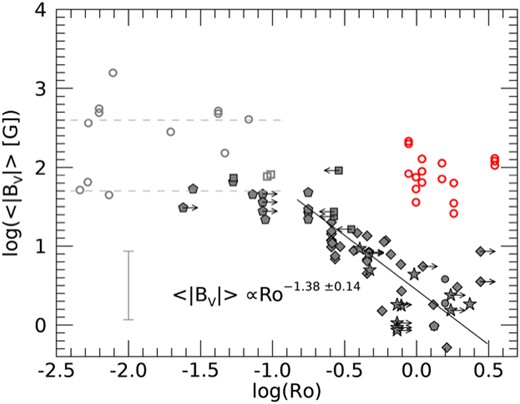
The averaged unsigned magnetic field strength 〈BV〉 versus Rossby number Ro as shown by Vidotto et al. (2014) (in grey scales) including our sample of slowly rotating M dwarfs (red circles). Note that for this figure only, we determined Ro using Wright et al. (2011) for consistency with Vidotto et al. (2014). For further details and the coloured version of the original symbols and annotations see fig. 4 a of Vidotto et al. (2014).
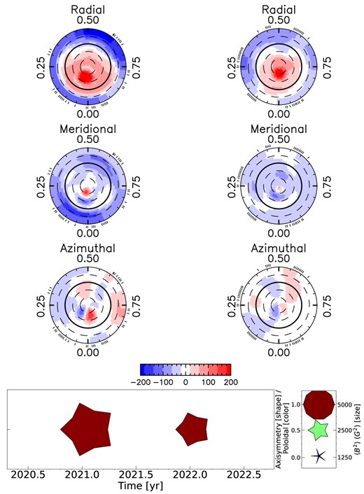
We stress that our paper focused on the most magnetic M dwarfs of the SLS sample (e.g. D23), whereas the other (less magnetic) stars of this sample will presumably be more in line with (and fill the gap between) the high-Ro stars of the Vidotto et al. (2014) sample. This will be the subject of forthcoming studies. Besides, our results suggest that the large-scale fields of the very slowly rotating M dwarfs of our sample are likely generated through dynamo processes operating in a different regime than those of the faster rotators that have been magnetically characterized so far. Fig. 20 summarizes the properties of the large-scale magnetic field topology for our six M dwarfs displaying all seasons on top of each other. It can be seen that the two partly convective M dwarfs (Gl 617B and Gl 408) show a smaller range of variations compared to the fully convective stars. The fully convective M dwarfs host large-scale fields that evolve on time-scales comparable to their rotation periods. Our small sample suggests that fully convective, slowly rotating M dwarfs tend to have large-scale fields that are less axisymmetric than their more massive counterparts.
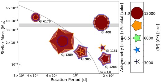
A summary of the magnetic properties of our M dwarf sample as a function of stellar mass and rotation period. The symbol size indicates the magnetic energy, the colour the poloidal fractional energy fpol, and the shape the axisymmetric fractional energy faxi (see the legend on the right). For each star, we display two to three symbols representing the individual seasons (blue, grey, and orange border for the first, second, and third season) of each M dwarf. The thin grey line indicates Ro = 1 determined using the empirical relation of Wright et al. (2018). The thick grey line marks the fully convection limit at |$M \approx 0.35\,$| M⊙.
In conclusion, we have analysed six slowly rotating M dwarfs observed by the SLS over 3.5 yr. We find that the large-scale magnetic field of these M dwarfs is unusually strong despite their slow rotation (40–190 d) and suggest that the efficiency of the dynamo for mid and late M dwarfs depends on Ro in a different way than that reported in the literature for faster rotators. Furthermore, we find that the large-scale magnetic field topology of the fully convective M dwarfs exhibit a larger range of variations than those of the two partly convective targets of our sample. Given this, it may be useful in the future to apply the time-dependent ZDI (Finociety & Donati 2022), which has only been tested for faster rotating stars up to now. We detected a polarity reversal on one (GJ 1151) and possibly two (Gl 905) of the four fully convective stars of our sample, suggesting that magnetic cycles may indeed be occurring in such stars, as initially suggested by Route (2016) from radio observations. Further long-term observations of the same type are needed to document in a more systematic fashion the long-term evolution of the large-scale magnetic fields of M dwarfs, and whether these field topologies are varying cyclically like for the Sun or in a more random fashion.
ACKNOWLEDGEMENTS
We acknowledge funding from the European Research Council (ERC) under the H2020 research & innovation programme (grant agreement #740651 NewWorlds). AC acknowledges funding from the French ANR under contract number ANR18CE310019 (SPlaSH). This work is supported by the French National Research Agency in the framework of the Investissements d’Avenir program (ANR-15-IDEX-02), through the funding of the ‘Origin of Life’ project of the Grenoble-Alpes University. AAV acknowledges funding from the European Research Council (ERC) under the European Union’s Horizon 2020 research and innovation programme (grant agreement no. 817540, ASTROFLOW). Our study is based on data obtained at the CFHT, which is operated by the CNRC (Canada), INSU/CNRS (France), and the University of Hawaii. The authors wish to recognize and acknowledge the very significant cultural role and reverence that the summit of Maunakea has always had within the indigenous Hawaiian community. We are very fortunate to have the opportunity to conduct observations from this mountain and gratefully acknowledge the CFHT QSO observers. This work has used astropy (Astropy Collaboration 2013, 2018, 2022), numpy (Harris et al. 2020), matplotlib (Hunter 2007), scipy (Virtanen et al. 2020), and benefited from the SIMBAD CDS data base and the ADS system.
DATA AVAILABILITY
All data underlying this paper are part of the SLS, and will be publicly available from the Canadian Astronomy Data Center by 2024 February.
References
APPENDIX A: ADDITIONAL GPR FITS INFORMATION AND FIGURES
Table A1 presents the ephemeris used for our M dwarf sample.
The ephemeris data used to determine the phases (|$\mathrm{phase} = \frac{T_0 -T_{\mathrm{obs}}}{P_{\mathrm{rot}}}$|) for the six M dwarfs of our sample. For T0 we used the barycentric Julian date of the first SPIRou observation of the target (second column). The last column indicates the rotation period Prot used for the phase determination.
| Star | T0 (JD) | Prot (d) |
|---|---|---|
| Gl 905 | 2458600.1348284 | 114.3 |
| GJ 1289 | 2458648.9872293 | 73.66 |
| GJ 1151 | 2458828.1234878 | 175.6 |
| GJ 1286 | 2458745.8452793 | 178.0 |
| Gl 617B | 2458744.743105 | 40.4 |
| Gl 408 | 2458590.0269338 | 171.0 |
| Star | T0 (JD) | Prot (d) |
|---|---|---|
| Gl 905 | 2458600.1348284 | 114.3 |
| GJ 1289 | 2458648.9872293 | 73.66 |
| GJ 1151 | 2458828.1234878 | 175.6 |
| GJ 1286 | 2458745.8452793 | 178.0 |
| Gl 617B | 2458744.743105 | 40.4 |
| Gl 408 | 2458590.0269338 | 171.0 |
For the GPR fits we used uniform |$\mathcal {U}$|, normal |$\mathcal {N}$|, and Jeffreys |$\mathcal {J}$| prior distributions. Table A2 indicates the prior used for Prot and the decay time l. For the smoothing factor, we use in general |$\mathcal {U}(0.1,1.0)$| beside for the GPR fits of GJ 1151 (|$\mathcal {U}(0.2,0.6)$|) and Gl 617B (|$\mathcal {U}(0.4,0.8)$|). For the amplitude α, we applied |$\mathcal {U}(0,\infty)$| with an exception for the GPR fits of GJ 1289 (|$\mathcal {N}(25,10)$|) and GJ 1286 (|$\mathcal {N}(16.4,5)$|). For the white noise, we used in general |$\mathcal {U}(0,\infty)$| beside for Gl 905, where we applied a Jeffreys priori distribution |$\mathcal {J}(1.5,\infty)$| for the GP fits.
The prior distribution used for the QP GPR fits for the rotation period Prot and decay time l.
| Star | Prior Prot (d) | Prior l (d) |
|---|---|---|
| Gl 905 | |$\mathcal {N}(115,20)$| | |$\mathcal {N}(130,25)$| |
| GJ 1289 | |$\mathcal {N}(75,5)$| | |$\mathcal {U}(50,1000)$| |
| GJ 1151 | |$\mathcal {N}(175,20)$| | 300 |
| GJ 1286 | |$\mathcal {N}(170,20)$| | 300 |
| Gl 617B | |$\mathcal {N}(40.4,5)$| | |$\mathcal {U}(30,1000)$| |
| Gl 408 | |$\mathcal {N}(170,15)$| | 200 |
In following, we present the corner plots of all QP GPR fits applied in this paper (see Fig. A1–A6).

The posterior density resulting from the MCMC sampling of the QP best-fitting GPR model for c1 (top) and Bℓ (bottom) for Gl 905. The concentric circle within each panel indicate the 1σ, 2σ, and 3σ contours of the distribution. The blue solid lines mark the mode (maximum) of the posterior distribution and the black dashed lines the median and the 16 per cent and 84 per cent percentiles of the posterior probability density function (PDF).
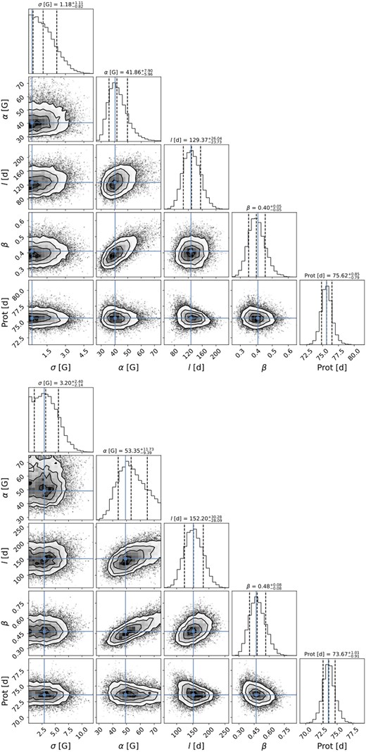
Same as Fig. A1 for GJ 1289.
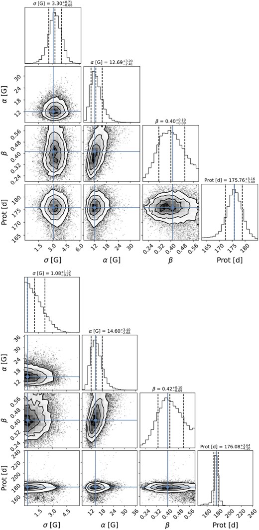
Same as Fig. A1 for GJ 1151.
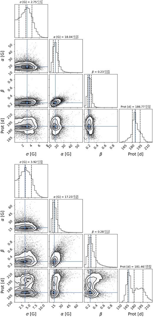
Same as Fig. A1 for GJ 1286.
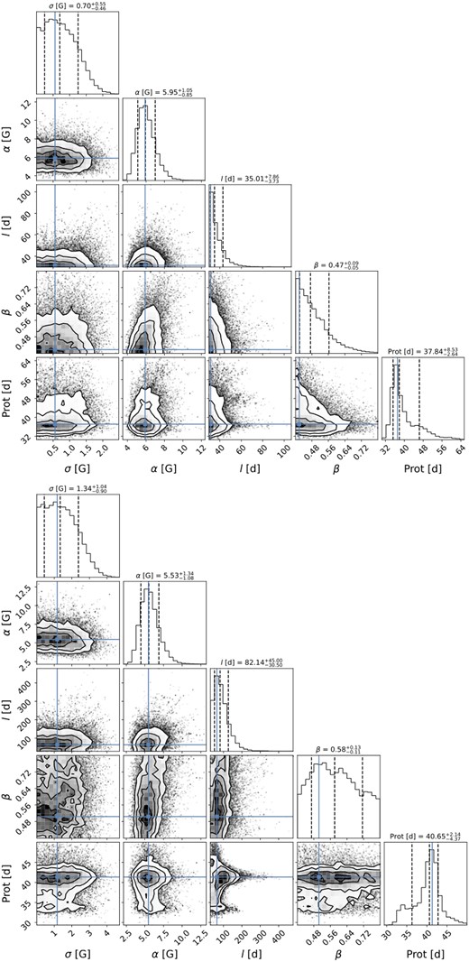
Same as Fig. A1 for Gl 617B.
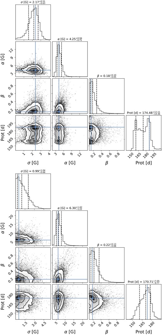
Same as Fig. A1 for Gl 408.
APPENDIX B: THE GPR FITS OF THE LONGITUDINAL FIELD VALUES
Table B1 provides a comparison of the GP results for c1 and Bℓ obtained with the GPR framework presented in Section 3.2 and the GP results of D23 for the Bℓ values (marked by D23 in the second column). For the GP fits the mean value is fixed to the Bℓ mean values determined by D23 for both c1 and Bℓ. Within the error, all three GP results agree for Prot, l, β, and α for each M dwarf, confirming Prot, l, β, and α using two different variables and calculation routines with one exception for Gl 617B, where the decay time determined from c1 differs from the GP results of Bℓ. The additional white noise σ is also consistent for both Bℓ, while c1 often shows lower σ values. Our GP routines fit the Bℓ data with a slightly higher or equal |$\chi ^2_r$| compared to the results of D23, while obtaining lower σ values. Comparing the results for c1 and Bℓ, we find that c1 has a lower rms. The rms of c1 and Bℓ is for all M dwarfs lower than the corresponding averaged error of c1 and Bℓ. For M dwarfs with significant non-axisymmetric field (e.g. Gl 905, GJ 1289, GJ 1286), c1 is fitted with lower or equal |$\chi ^2_r$| and can provide smaller errors for Prot (e.g. GJ 1289, GJ 1286). For M dwarfs with highly axisymmetric fields (e.g. Gl 617B, Gl 408), Bℓ gives smaller errors on Prot.
Summary of the best-fitting parameters of the QP GPR fits applied to c1 and Bℓ for the six M dwarfs in our sample and the comparison with the corresponding GPR results for Bℓ by D23 marked as D23 in the second column.
| Star | Data | Rotation period | Decay time | Smoothing factor | Amplitude | White noise | Rms | |$\chi ^2_{\rm r}$| |
|---|---|---|---|---|---|---|---|---|
| Prot (d) | l (d) | β | α (G) | σ (G) | (G) | |||
| Gl 905 | c1 | |$111.7^{+3.0}_{-3.2}$| | |$133^{+18}_{-22}$| | |$0.50^{+0.09}_{-0.07}$| | |$12.9^{+3.1}_{-2.1}$| | |$0.6^{+0.5}_{-0.4}$| | 3.8 | 0.79 |
| Gl 905 | Bℓ | |$114.4^{+3.5}_{-2.4}$| | |$130^{+25}_{-32}$| | |$0.44^{+0.12}_{-0.09}$| | |$14.1^{+3.5}_{-2.4}$| | |$1.2^{+1.1}_{-0.8}$| | 6.9 | 0.87 |
| Gl 905 | D23 | 114.3 ± 2.8 | |$129^{+25}_{-21}$| | 0.43 ± 0.09 | |$13.3^{+2.5}_{-2.1}$| | |$1.7^{+1.2}_{-0.7}$| | 6.2 | 0.84 |
| GJ 1289 | c1 | |$75.62^{+0.85}_{-0.79}$| | |$129^{+26}_{-24}$| | 0.40 ± 0.05 | |$41.9^{+7.9}_{-6.0}$| | |$1.2^{+1.1}_{-0.8}$| | 6.9 | 0.72 |
| GJ 1289 | Bℓ | |$73.67^{+1.01}_{-0.91}$| | |$152^{+30}_{-28}$| | 0.48 ± 0.08 | |$53.3^{+11.7}_{-9.4}$| | |$3.2^{+2.4}_{-2.1}$| | 14.3 | 0.84 |
| GJ 1289 | D23 | 73.66 ± 0.92 | |$152^{+32}_{-27}$| | 0.48 ± 0.09 | |$53.2^{+12.4}_{-10.1}$| | |$4.2^{+2.7}_{-1.6}$| | 13.9 | 0.82 |
| GJ 1151 | c1 | |$175.8^{+3.2}_{-3.4}$| | 300 | |$0.40^{+0.10}_{-0.09}$| | |$12.7^{+3.2}_{-2.4}$| | 3.3 ± 0.7 | 5.8 | 0.99 |
| GJ 1151 | Bℓ | |$176.1^{+3.6}_{-4.1}$| | 300 | |$0.42^{+0.10}_{-0.09}$| | |$14.6^{+3.4}_{-2.7}$| | |$1.1^{+1.1}_{-0.8}$| | 6.7 | 0.73 |
| GJ 1151 | D23 | 175.6 ± 4.9 | 300 | 0.43 ± 0.11 | |$14.9^{+4.2}_{-3.3}$| | |$1.6^{+1.3}_{-0.7}$| | 6.7 | 0.72 |
| GJ 1286 | c1 | |$186.8^{+9.5}_{-5.8}$| | 300 | |$0.23^{+0.05}_{-0.04}$| | |$18.0^{+4.3}_{-3.1}$| | |$2.7^{+1.5}_{-1.7}$| | 7.5 | 1.02 |
| GJ 1286 | Bℓ | |$181^{+18}_{-13}$| | 300 | |$0.28^{+0.13}_{-0.07}$| | |$17.2^{+6.2}_{-3.6}$| | |$3.9^{+2.3}_{-2.4}$| | 12.0 | 1.03 |
| GJ 1286 | D23 | 178 ± 15 | 300 | 0.29 ± 0.09 | |$16.7^{+4.6}_{-3.6}$| | |$4.6^{+2.6}_{-1.6}$| | 10.1 | 1.02 |
| Gl 617B | c1 | |$37.8^{+8.5}_{-2.6}$| | |$35^{+8}_{-4}$| | |$0.47^{+0.09}_{-0.05}$| | |$5.9^{+1.2}_{-0.8}$| | |$0.7^{+0.6}_{-0.5}$| | 2.2 | 0.66 |
| Gl 617B | Bℓ | |$40.6^{+2.1}_{-4.4}$| | |$82^{+45}_{-30}$| | |$0.58^{+0.13}_{-0.11}$| | |$5.5^{+1.3}_{-1.1}$| | |$1.3^{+1.0}_{-0.9}$| | 5.0 | 0.86 |
| Gl 617B | D23 | 40.4 ± 3.0 | |$69^{+35}_{-23}$| | 0.60 ± 0.22 | |$5.4^{+1.3}_{-1.0}$| | |$1.7^{+1.1}_{-0.7}$| | 4.9 | 0.86 |
| Gl 408 | c1 | |$175^{+12}_{-14}$| | 200 | |$0.18^{+0.10}_{-0.05}$| | |$4.2^{+0.9}_{-0.8}$| | |$2.2^{+0.5}_{-0.6}$| | 3.9 | 1.19 |
| Gl 408 | Bℓ | |$170.7^{+7.1}_{-9.8}$| | 200 | |$0.22^{+0.13}_{-0.08}$| | |$6.3^{+1.6}_{-1.2}$| | |$1.0^{+1.0}_{-0.7}$| | 6.9 | 0.72 |
| Gl 408 | D23 | 171.0 ± 8.4 | 200 | 0.21 ± 0.10 | |$6.3^{+1.5}_{-1.2}$| | |$1.5^{+1.2}_{-0.7}$| | 6.3 | 0.66 |
APPENDIX C: ADDITIONAL PCA AND ZDI FIGURES
We can confirm that the symmetric component (with respect to the line centre) seen in the mean profile of the 2020/21 season for Gl 905 is due to the irregular phase coverage of the observations and does not reflect an axisymmetric toroidal field. We simulated 24 equally spaced Stokes V LSD profiles from the 2020/21 ZDI map (Fig. 3 middle column). The symmetric component of the resulting mean profile disappears for the uniform phase coverage (see Fig. C1). None the less, we might still miss toroidal field due to the low vesin i, see the |$\sigma _{\langle B_\mathrm{tor} \rangle }$| estimation in Section 4.2.
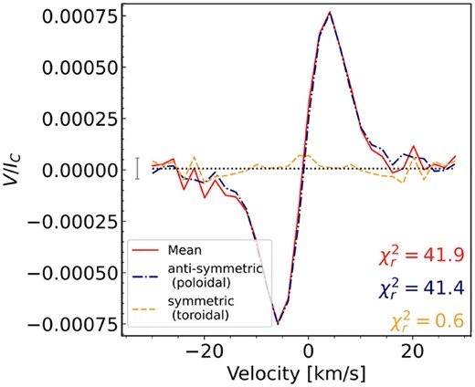
The mean profile and its decompositions obtained from 24 uniformly phased synthetic Stokes V LSD profiles of the 2020/21 ZDI map of Gl 905. The same format as in Fig. 1(a) is used.
Figs C2 and C3 show the ZDI maps of Gl 617B and Gl 408 for an alternative inclination i = 30°.
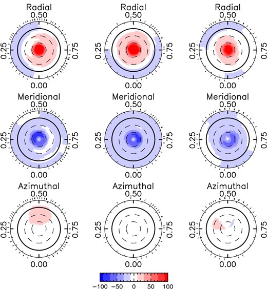
The magnetic field maps of Gl 617B using an inclination i = 30° presented in the same format as in Fig. 3.
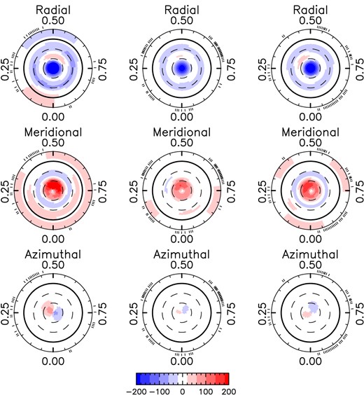
The magnetic field maps of Gl 408 using an inclination i = 30° presented in the same format as in Fig. 3.
The following figures (Fig. C4–C9) display the observed Stokes V LSD profiles (black) and their ZDI fits (red) split by season for the six M dwarfs.
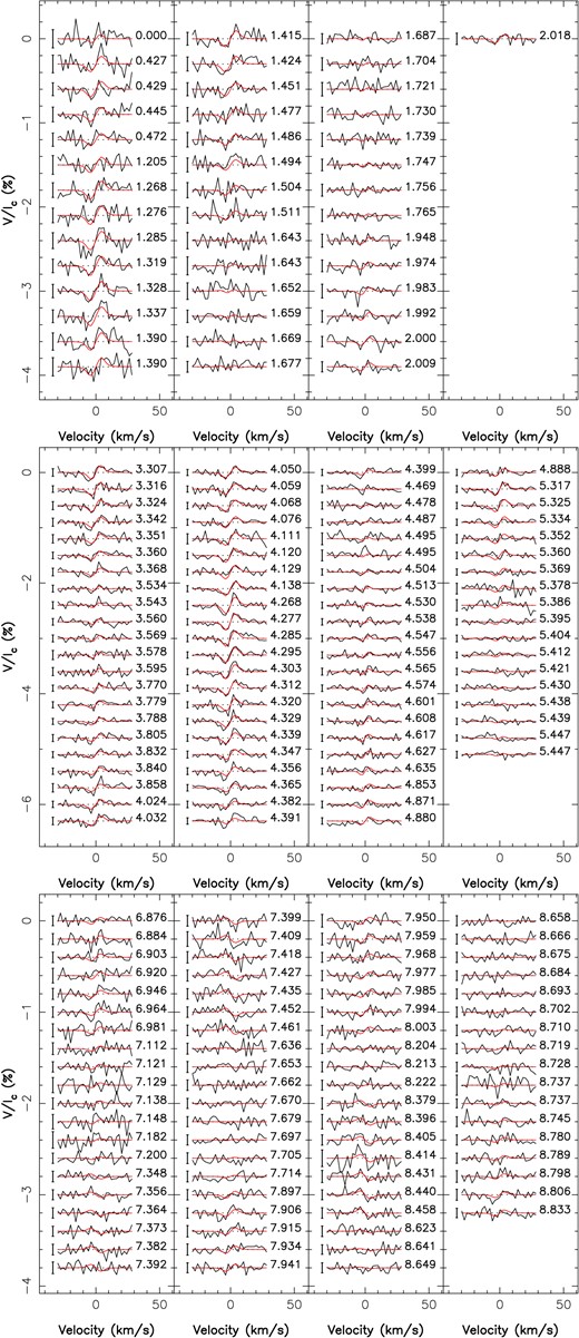
The SPIRou observed LSD Stokes V profiles (black) and the ZDI fit (red) for Gl 905. The rotation phase is indicated to the right of the profile and the error to the left. Each panel corresponds to one season.

Same as Fig. C4 for GJ 1289.
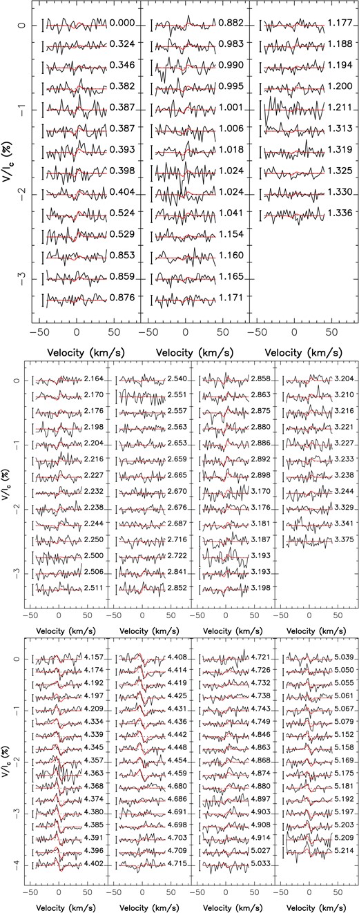
Same as Fig. C4 for GJ 1151.
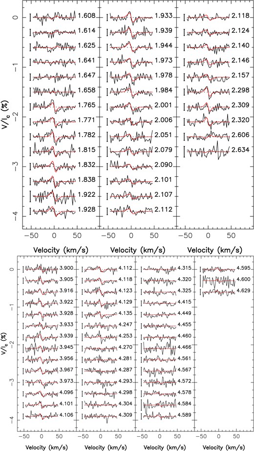
Same as Fig. C4 for GJ 1286.
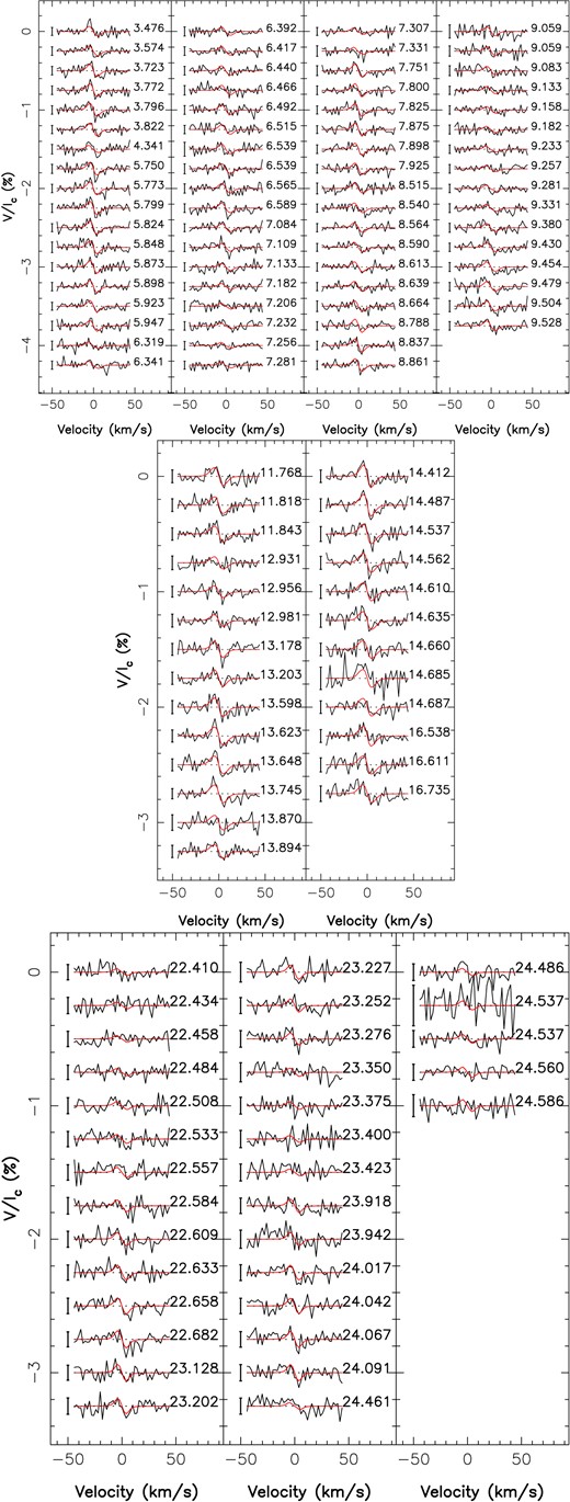
Same as Fig. C4 for Gl 617B.
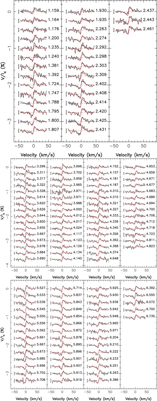
Same as Fig. C4 for Gl 408.
