


ABSTRACT
Starting from the Gaia DR3 HR diagram, we derive the star formation history (SFH) as a function of distance from the Galactic plane within a cylinder centred on the Sun with a 200 pc radius and spanning 1.3 kpc above and below the Galaxy’s midplane. We quantify both the concentration of the more recent star formation in the Galactic plane, and the age-related increase in the scale height of the Galactic disc stellar component, which is well-described by power laws with indices ranging from 1/2 to 2/3. The vertically-integrated star formation rate falls from |$(1.147 \pm 0.039)\times 10^{-8}\, \text{M}_\odot \, \text{yr}^{-1} \, \text{pc}^{-2}$| at earlier times down to |$(6.2 \pm 3.0) \times 10^{-9}\, \text{M}_\odot \, \text{yr}^{-1} \, \text{pc}^{-2}$| at present times, but we find a significant peak of star formation in the 2–3 Gyr age bin. The total mass of stars formed per unit area over time is |$118.7 \pm 6.2\, \text{M}_\odot \, \text{pc}^{-2}$|, which is nearly twice the present stellar mass derived from kinematics within 1 kpc from the Galactic plane, implying a high degree of matter recycling in successive generations of stars. The method is then modified by adopting an age-dependent correlation between the SFH across the different slices, which results in less noisy and more symmetrical results without significantly changing the previously mentioned quantities. This appears to be a promising way to improve SFH recovery in external galaxies.
1 INTRODUCTION
Thanks to the Gaia DR3 catalogue (Gaia Collaboration et al., 2016; Gaia Collaboration et al, 2023j), the Milky Way (MW) is now the only galaxy where the 3D distribution of stars can be precisely mapped across distances of a few kiloparsecs with resolution of a few tens of parsecs. Such a precise mapping is changing the perspective for stellar population studies: our specific position inside the MW is no longer ‘a complication’ in the analysis of global properties of the MW, but might eventually become an advantage, allowing us to fully understand the geometry of its stellar populations and dust–hence allowing for a better understanding of the populations that we are seeing, projected in 2D, in external disc galaxies.
Deriving the geometry of nearby stellar populations from Gaia, and especially their vertical distribution, perpendicular to the Galactic plane, is indeed the goal of many recent papers (e.g. Bovy 2017; Li & Widrow 2021; Yu et al. 2021; Everall et al. 2022; Robin et al. 2022; Widmark, Widrow & Naik 2022). These works make use of a variety of different techniques, applied to particular stellar tracers from Gaia, often taking advantage of their rich kinematic information and of the modelling of the MW gravitational potential.
In addition, the precise photometry of the Gaia catalogue enables the construction of the colour-absolute magnitude diagram (CAMD), thus providing crucial information on the stellar ages. Fitting this diagram with theoretical models of stellar populations allows us to derive the star formation history (SFH) in selected volumes, as done by, e.g. Gallart et al. (2019), Ruiz-Lara et al. (2020), Alzate, Bruzual & Díaz-González (2021), and Dal Tio et al. (2021), using different methods and different sample sizes. There are also more complete attempts to derive both the SFH and structural parameters of the Galactic disc via population synthesis and kinematic modelling aimed to reproduce Gaia data, as is the case of Mor et al. (2019), Sysoliatina & Just (2022), and Robin et al. (2022).
In this work, we attempt a different kind of analysis of Gaia data to derive the SFH of the extended solar neighbourhood. We consider a sample of stars in a cylindrical volume spanning approximately 1300 pc above and below the Galactic plane, with its axis normal to the plane and passing through the Sun. We slice it in layers along its axis and fit simultaneously the CAMD of all slices, using a modified version of the SFH-recovery method routinely applied to nearby galaxies. Our main goal is to map the vertical distribution of stellar populations of different ages, in a self-consistent way, to infer their relative contributions to the local disc density and their vertical distribution as a function of age. At the same time, we aim to derive the integrated properties of the MW disc close to the Sun, as would be seen by a distant observer. Last but not least, we have the long-term goal of improving the tools available for the analysis of SFHs in galaxies, and checking the assumptions that have been widely adopted in the study of external galaxies.
The structure of this paper is as follows: Section 2 describes the Gaia DR3 data used in this work. Section 3 describes how the stellar populations are modelled considering the selection effects present in Gaia. Section 4 describes the numerical method used to derive the SFH in every region analysed. Section 5 then discusses the results in terms of the age and spatial distribution of the SFH results. Section 6 attempts to further improve the results via a new method that assumes a spatial correlation in the SFHs at different locations. Section 7 summarizes the main conclusions.
2 DATA
2.1 Building the sample
The initial sample of stars we download from the Gaia archive is composed of all sources located in a sphere of radius 1.5 kpc centred on the Sun. We use the query presented in the Appendix A of the online supplementary material, with rmax = 1500 pc.
The sample collected in this way is initially filtered to include only stars that fall inside a cylinder of radius Rmax = 200 pc and height H = 2.6 kpc, spanning H/2 = 1.3 kpc above and below the Galactic plane. The Rmax = 200 pc ensures small variations in the mean properties of stellar populations across its 400 pc total range of Galactocentric radius: indeed, the change in mean metallicities due to the radial metallicity gradient in the Galactic disc should be smaller than 0.014 dex (assuming the radial gradient of −0.07 dex kpc−1; Rolleston et al. 2000), and the local stellar density should change by less than 15 per cent (given a scale length for the thin disc of 2600 pc; Jurić et al. 2008). The maximum height of H/2 = 1.3 kpc is large enough to include at least one scale height of the oldest disc populations (approximately 900 pc; Jurić et al. 2008; Pieres et al. 2020), and small enough to ensure high completeness and small parallax errors (see Section 3.1 below).
An important consideration is that the Sun is not located exactly at the Galactic midplane. Studies consistently find a 15–20 pc offset between the midplane and the Sun. For example, Karim & Mamajek (2017), using Galactic disc tracer objects estimated that z⊙ = 17 ± 5 pc. Siegert (2019) determined the solar offset to be z⊙ = 15 ± 17 pc using γ-rays. Joshi & Malhotra (2022) used open clusters younger than 700 Myr and found that the solar offset amounts to z⊙ = 17.0 ± 0.9 pc. Griv et al. (2021) determined a value of z⊙ = 20 ± 2 pc from Type II Cepheids, slightly larger than the other estimates. In this paper, we adopt the weighted average of these results, and use z⊙ = 17.7 pc. We then compute the Cartesian coordinates (x, y, z) of the stars in our initial sample as
where (l, b) are the Galactic coordinates of each source and r is the distance of the source from the Sun (see Section 2.2). We keep in our sample only the stars inside the solar cylinder, which we define using the following conditions:
After selecting stars in the cylinder, we turn to the selection of stars based on the quality of their photometry. Riello et al. (2021) have shown that the Gaia photometric excess factor in the GBP and GRP bands [phot_bp_rp_excess_factor, corrected using their equation (6)] is a measure of the consistency between the photometric measurements in the three Gaia bands, a key requirement for this study given the crucial role of the Gaia CAMD. Therefore, we filter the sample according to Section 9 of Riello et al. (2021). This filtering might eliminate high-amplitude variable stars and extended sources, in addition to stellar sources with suspicious photometry. Fig. 1 shows the fraction of stars retained as a function of apparent G-band magnitude in the whole cylinder, near the Galactic plane, and on the far sides of the Cylinder. The bottom panel of Fig. 2 shows the Hess diagram, which is the 2D histogram of the CAMD, of sources lost over the whole cylinder. To minimize the number of sources removed from the sample, we apply no other data quality cuts.
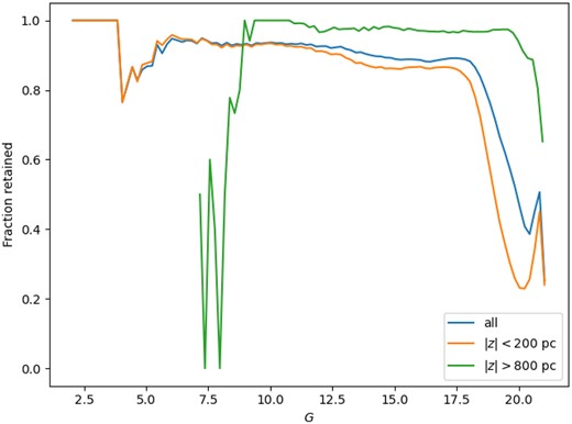
Fraction of stars retained in the sample after the cut on phot_bp_rp_excess_factor versus apparent G magnitude for different intervals of z: the full cylinder, |z| < 1315.78 pc (blue); |z| < 200 pc (orange); |z| > 800 pc (green). It should be noted that in the case |z| > 800, only about 0.1 per cent of the stars have G < 10 mag.
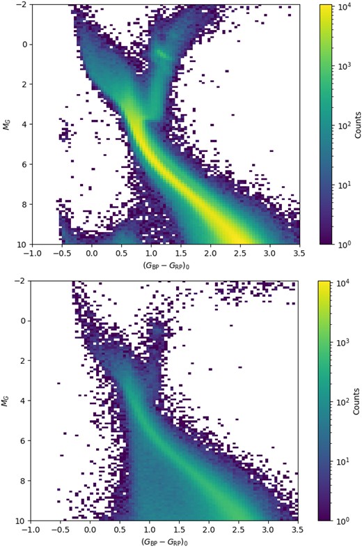
Upper panel. Hess diagram of all the sources that were kept in the sample (5128792) based on the phot_bp_rp_excess_factor selection. Lower panel. Same as above, but for all the sources that were removed from the sample (1594031) based on the phot_bp_rp_excess_factor selection. For both diagrams, the size of the bins is 0.1 mag in magnitude and 0.05 mag in colour. A clear feature can be seen in the upper panel at 3.5 ≲ MG ≲ 5 and (GBP − GRP)0 ≈ −0.5, which corresponds to the locus of the hot subdwarf stars, a product of binary evolution.
2.2 Distance and extinction
We use the distances provided by the inverse of the Gaia DR3 parallax, since it represents a quite direct measurement with a clear definition of its error, which can be quite easily replicated in our models (see Section 3.1 below).
We computed parallax zero-point corrections following the prescriptions from Lindegren et al. (2021).1 However, we found that the median value of the absolute change in parallax resulting from correcting our sample is less than 1 per cent, and that about 90 per cent of the stars in the sample have their parallaxes corrected by less than 2 per cent. Given the small impact of the correction and the way we include parallax errors in our models, we decided not to apply it. This simplification is justified by the relatively small distance of all stars in our sample. The zero-point correction could not be neglected were the sample to be extended over longer distances.
For the extinction, we adopt the 3D extinction map from Vergely, Lallement & Cox (2022). These authors devised a novel technique that allowed them to inter-calibrate different extinction catalogues and to obtain a 3D extinction density map via a hierarchical inversion technique with different volume and spatial resolution.2 In view of possible expansions of this work to larger distances, we chose the map that covers a volume of 6000 × 6000 × 800 pc with a resolution of 25 pc. This map is available at the CDS3 and stores the extinction density at 550 nm (A0). To determine the extinction of a star at a certain distance, we integrate the extinction density along the line of sight to the star and convert the value to Gaia magnitudes using the simple relation
where X is one of G, GBP, and GRP, and
are the values suitable for a yellow dwarf in the regime of low extinction, computed for the Gaia EDR3 photometric system as in Girardi et al. (2008), using the O’Donnell (1994) mean interstellar extinction curve with RV = 3.1. Then, we subtract the expected values of extinction from the magnitudes of the stars. In the whole sample, we find a maximum value of A0 = 0.89 mag, and close to the Galactic plane (|z| < 50 pc) more than 75 per cent of the stars have A0 < 0.15 mag.
The resulting CAMD is shown in the top panel of Fig. 2 in the form of a Hess diagram, i.e. a two-dimensional histogram built from the colours and magnitudes of the stars in our sample.
2.3 Slicing the data
As we aim to determine the vertical structure of the SFH, we slice our cylindrical sample of stars into thin slices parallel to the Galactic plane (hereafter referred to simply as ‘slices’). More specifically, we split the sample in 28 slices with Δz ≈ 50 pc for |z| < 158 pc and Δz ≈ 100 pc for |z| > 158 pc. The exact intervals in z assigned to each slice are listed in Table 1.
Intervals of z covered by each slice of the initial sample on the Northern side (z > 0) of the Galactic plane, such that zmin ≤ z ≤ zmax. The same scheme is repeated on the opposite side (z < 0).
| zmin [pc] | zmax [pc] |
|---|---|
| 0.00 | 52.63 |
| 52.63 | 105.26 |
| 105.26 | 157.89 |
| 157.89 | 263.16 |
| 263.16 | 368.42 |
| 368.42 | 473.68 |
| 473.68 | 578.95 |
| 578.95 | 684.21 |
| 684.21 | 789.47 |
| 789.47 | 894.74 |
| 894.74 | 1000.00 |
| 1000.00 | 1105.26 |
| 1105.26 | 1210.52 |
| 1210.52 | 1315.78 |
The reason why we chose this layout, with smaller heights near the Galactic plane, is to improve the resolution at lower z, where the number of stars is substantially larger than at larger distances from the plane of the Galaxy.
3 MODELS
3.1 Creating partial models for single stars
Partial models (PM) are Hess diagrams of simple stellar populations covering limited ranges of age and metallicity. In the case of single stars, they are built using the TRILEGAL code (Girardi et al. 2005) with the same approach as in Dal Tio et al. (2021, see their fig. 4): population models are computed for seven values of mean metallicity around a reference age–metallicity relation (AMR), and for 16 age bins. The age bins are 0.2 dex wide in log (t[yr]), with the exception of the first age bin that spans 0.5 dex, overall providing a good balance between high enough statistics (even for the sparsely-populated slices far from the Galactic plane) and age resolution.
The partial models are based on PARSEC v1.2S evolutionary tracks (Bressan et al. 2012; Chen et al. 2014) and comprise the synthetic photometry in the Gaia DR3 filter transmission curves. They are also normalized to a constant star formation rate (SFR) of 1 M⊙ yr−1 over their age interval, assuming the Kroupa (2002) initial mass function. Examples of partial models for single stars built in this way are presented in Appendix C of the online supplementary material.
As such, these initial partial models do not include the errors and incompleteness that characterize the real Gaia data. In the classical works of SFH analysis (see e.g. Mazzi et al. 2021, and references therein), the completeness and photometric errors are derived via artificial star tests (ASTs): one injects huge numbers of fake stars in the original images and then recovers them using the same photometry pipeline used for the real data. Then, for every position in the colour-magnitude diagram, one derives the distribution of errors as the differences between the input and output colours and magnitudes, and the completeness as the number of recovered stars compared to the input fake stars. These quantities are a function of the sky position. They are then applied to the partial models, which represent a complete sample of model stars.
It is obvious that the procedure has to be different for Gaia data because its photometry and astrometry do not simply derive from CCD images, but from a complex observational procedure and data analysis pipeline (see Gaia Collaboration et al. 2021a; van Leeuwen et al. 2022, and references therein). Fortunately, the errors and incompleteness of the Gaia DR3 catalogue have been characterized extensively in a series of papers. In the present analysis, we adopt the following procedure, which represents an extension and update of the one used by Dal Tio et al. (2021):
For every slice of the cylinder as defined in Table 1, we generate random positions (R, z) for 2 million fake stars with constant density within the limits of R < Rmax + δRmax and zmin − δz < z < zmax + δz, where δRmax = 0.2Rmax and δz = 0.1(zmax − zmin). We generate fake stars in a volume larger than each slice because parallax errors open the possibility that stars generated within the R < Rmax and zmin < z < zmax limits are ‘observed’ slightly outside it; conversely, stars slightly outside the slice can be inserted into the sampled region. We compute the parallax of every fake star from their distances from the Sun, and apply fake errors to its parallax. These errors are derived from the parallax errors reported in the Gaia DR3 catalogue, for every slice, following the procedure outlined in Appendix B of the online supplementary material.
Every fake star is assigned a random absolute magnitude and colour within −2 < MG < 12 and −1.2 < (GBP − GRP)0 < 4, respectively. These limits are kept, intentionally, wider than the data we actually analyse in the end. The absolute magnitudes are then converted to apparent magnitudes using the fake parallaxes computed in (i) and are subsequently degraded applying the typical errors in G, GRP, and GBP determined from the Gaia catalogue as outlined in Appendix B of the online supplementary material.
The apparent magnitudes and sky coordinates of every fake star are provided as input to the GaiaUnlimited python module for the completeness of the Gaia catalogue (Cantat-Gaudin et al. 2023), which computes the probability P of observing each fake star in Gaia DR3. We use a randomly generated number p, between 0 and 1, to determine if the fake star is observed (p < P) or not (p > P).
The fake star experiments presented above are used to derive the distributions of errors in absolute magnitude and colour and the incompleteness for every small bin in the CAMD. In particular:
All stars generated inside the R < Rmax and zmin < z < zmax volume and the −2 < MG < 12 and −1.2 < (GBP − GRP)0 < 4 CAMD limits are counted as ‘input fake stars’, ninput.
All stars that are found, after their errors are simulated, inside the R < Rmax and zmin < z < zmax volume and the −2 < MG < 10 and −1 < (GBP − GRP)0 < 3.5 CAMD limits are counted as ‘observed stars’, nobserved, and contribute to the estimation of the colour and magnitude errors.
The completeness fraction is computed as C = nobserved/ninput.
We remark that the fake stars in the δz and δR regions allow us to estimate how much each partial model is affected by stars that are scattered inside/outside the sampled volume due to their parallax errors. For a volume centred on the Sun, the probability of stars being scattered inwards is slightly higher than the probability of stars being scattered outwards.4 Therefore, this opens the possibility of finding completeness fractions C exceeding the value of 1 in some cases. For the present choice of parameters, the maximum values of C are of 1.007, and C > 1 values are found in the partial models of slices closer to the Galactic plane.
Fig. 3 illustrates the results of such ASTs for a few cases: the slice closer to the Sun (|$0.00 \, \text{pc} < z < 52.63 \, \text{pc}$|); three intermediate ones (|$368.42 \,{\rm pc} < z < 473.68 \,{\rm pc}$|, |$684.21 \, \text{pc} < z < 789.47 \, \text{pc}$| and |$894.74 \, \text{pc} < z < 1000.00 \, \text{pc}$|); and the most distant one (|$1210.52 \, \text{pc} < z < 1315.78 \, \text{pc}$|). In the first case, completeness is extremely high, except for a moderate loss of stars at MG ≲ 0 because of their saturation.5 In the following cases, completeness progressively decreases until, in the furthest slice, no fewer than about 10 per cent of the stars are lost at all magnitudes, with this fraction increasing rapidly at MG ≳ 4. This limit is a consequence of the combination of incompleteness as determined by GaiaUnlimited and the increase in photometric errors for fainter sources. In all the cases presented above, photometric errors are very small: for MG < 4, we find a median magnitude error of |$\sigma _{M_{\rm G}}=0.021$| mag and 99 per cent of the artificial stars have |$\sigma _{M_{G}} < 0.102$| mag. Similarly, the median error on the colour is |$\sigma _{(G_{\text{BP}}-G_{\text{RP}})_{0}}=0.0034$|, with 99 per cent of the artificial stars having |$\sigma _{(G_{\text{BP}}-G_{\text{RP}})_{0}} < 0.0141$|.
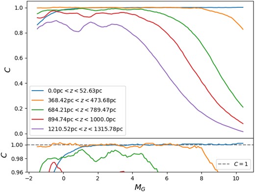
Results of the ASTs in five slices illustrate the trend of completeness with the MG magnitude. The lower panel zooms to the region with high completeness to highlight the occurrence of C > 1 for the slices closest to the Galactic plane.
Finally, these distributions of errors and completeness are applied to the original, ‘input partial models’, generating realistic ‘observed partial models’ for every slice.
3.2 Creating the partial models for binaries
For binaries, the above-mentioned procedure gains a new complication: binary components too close to the sky and with a too large contrast in magnitude are identified as a single star in the Gaia DR3 catalogue. This effect depends on the distance from the Sun, with distant samples having a larger fraction of unresolved binaries than nearby samples.
To take this factor into account, we adopt the same procedure as in Dal Tio et al. (2021): the BinaPSE module of the TRILEGAL code is used to generate coeval samples of binaries starting from the initial distribution of orbital parameters derived by Moe & Di Stefano (2017) and using the Kroupa (2002) IMF for the primary masses. These are our ‘binary partial models’: they have the same initial total mass as the single star partial models of the same age and metallicity and are normalized to a constant SFR of 1 M⊙ yr−1 as well. Then, BinaPSE follows the evolution of the binaries, both in their physical properties and in their orbital parameters. At the selected partial model age, we generate the magnitude contrast between the two components, as well as the expected separation of the binary members for a random epoch, random orientation of the orbit (i.e. for an isotropic distribution), and random position of the centre of mass inside the slice. If the combination of angular separation and magnitude contrast between the components turns out to be larger than the limits defined by equation (2) of Gaia Collaboration et al. (2021b) (which replaces the Ziegler et al. 2018 and Brandeker & Cataldi 2019 relations based on Gaia DR2), they are treated as two separated stars, each one with its own photometry. Otherwise, they are treated as a single object, with the photometry being computed by adding the fluxes of the two components. (or by the left-over star in the case of coalesced binaries). In both cases, the photometric errors and completeness already derived from single stars are applied to convert the input binary partial models into the final observed ones. Examples of binary partial models are provided in Appendix C of the online supplementary material.
It is worth pointing out the importance of accounting for both resolved and unresolved binary stars, especially when using Gaia data, even though they are often neglected in literature studies dealing with SFH recovery. While the detailed implications will be addressed in a forthcoming paper on the binary fraction of the solar neighbourhood, we can work out a simple instructive example comparing a binary partial model in a slice close to the plane and one at 1 kpc. Indeed, the number of objects in the latter one is about 6 per cent smaller than the former one, even though they refer to the same population of binaries. If not properly accounted for, the effect of resolvability is prone to propagating into the values derived for the absolute SFR and the binary fraction. Even more subtle effects may derive from the fact that the fraction of some binaries is a function of orbital separation. According to Moe & Di Stefano (2017), this happens for the ‘twins’, i.e. the binaries in which the two components have a similar initial mass, which are favoured at small periods. Since unresolved twins have a very distinct location in the CAMD, the incorrect simulation of their resolvability at different distances may also affect the residuals of the model fits across the CAMD.
3.3 Creating a partial model for the Galactic halo
It is well known that the solar vicinity is immersed in a low-density halo of old metal-poor stars, that can be followed spatially up to very large distances (e.g. Jurić et al. 2008), and which is responsible for a background of deep star counts over large areas of the sky (e.g. Pieres et al. 2020). This background of stars is expected to vary modestly and smoothly across our solar cylinder, and we can consider it as a fixed element in the fit of the Hess diagram. In this work, we adopt the TRILEGAL default halo model (Girardi et al. 2012) to create the halo population for every slice, and then apply the corresponding ASTs as described above, creating additional partial models called PM0.
3.4 Computing the total model and its likelihood
From the partial models described above, we can build a so called ‘total model’ for a slice as
where SFH is the star formation history of the slice, fbin is the binary fraction, which we define as the mass fraction of a stellar population initially born in the form of binaries, and ΔMG and Δ(GBP − GRP)0 are global shifts of the Hess diagram intended to take into account possible issues in the Gaia photometry or in the definition of the filters of the model. The SFH consists of two parts, the SFR as a function of age and the AMR, which describes how metallicity varies with age. We indicate by ai the value of the SFR in the i-th age bin, and by [Fe/H]i the corresponding value of metallicity. Finally, PM0 takes into account any additional contributions to the total Hess diagram that has to be kept fixed during the optimization. In our case, as discussed in Section 3.3, we choose to keep fixed the partial model of the Halo. However, in our testing, we find that including or excluding the Halo model does not change the result significantly.
In the computation of the total model, there are a few intermediate steps. First, we need to derive the models with the requested metallicity. We do so by interpolating between the sets of both single and binary partial models we computed for different metallicities. More specifically, we get the partial models at age i for the desired metallicity [Fe/H]i by interpolation:
where |$\mathrm{PM}_{i}^{-}$| and |$\mathrm{PM}_{i}^{+}$| are the partial models at metallicity |$[\text{Fe}/\text{H}]_{i}^{-}$| and |$[\text{Fe}/\text{H}]_{i}^{+}$|, respectively, and at the age i that bracket the target metallicity, and |$f_{i}=([\text{Fe}/\text{H}]_{i}-[\text{Fe}/\text{H}]_{i}^{-})/([\text{Fe}/\text{H}]_{i}^{+}-[\text{Fe}/\text{H}]_{i}^{-})$|. This allows us to compute a limited number of sets of partial models, thus reducing the time needed initially, but still be able to simulate the whole metallicity range. The second step consists in combining single and binary models at each age. Our definition of binary fraction fbin implies that at all ages and metallicities a SFR of 1 M⊙ yr−1 is represented by the sum of (1 − fbin) times the partial model for single stars, plus fbin times the partial model for binaries. Lastly, we combine the partial models at each age using the SFRs, ai, as weights to obtain the total model M. Putting these last two steps together, the total model is computed as
where PMsin, i and PMbin, i are the partial models for single and binary stars, respectively.
The main objective of our work is determining the set of parameters that minimizes the residuals between the model and the data for each slice of the cylinder. To evaluate how well a model produced by a given set of parameters compares to the data, we adopt a method similar to the ones presented in Dal Tio et al. (2021) and Mazzi et al. (2021). We adopt 16 age bins from log (t[yr]) = 6.6 to log (t[yr]) = 10.1, and compute models at those ages for a reference AMR (see fig. 4 in Dal Tio et al. 2021 and Fig. D1) and six additional sets at {−3, −2, −1, 1, 2, 3}Δ[Fe/H], where Δ[Fe/H] = 0.12 dex. Every set has an intrinsic spread in metallicity defined by a Gaussian of σ = 0.1 dex.
At a first glance, the parameters to fit for each slice are 16 ai, 16 [Fe/H]i, the binary fraction, and the two additional parameters describing the rigid shifts of the CAMD along the magnitude and colour axes, ΔMG and Δ(GBP − GRP)0. With 28 slices of data, the total number of parameters that have to be explored is 980.
To reduce the size of the problem, we can make a few assumptions:
In our solar cylinder sample, we do not expect the binary fraction fbin to change with the height from the Galactic plane therefore we can fit a single value for all slices.
Similarly, we do not expect ΔMG and Δ(GBP − GRP)0 to change with z, and we can fit only one value of each parameter for the whole sample.
For the AMR, the observed vertical metallicity gradient of the disc, i.e. the trend of finding lower [Fe/H] values at high |z| (see, e.g. fig. 4 in Hayden et al. 2015, and Appendix D of the online supplementary material), might be the simple result of having young, metal rich populations being confined at low |z|, while old metal poor stars dominate the star counts at high |z|. As we are exploring the age structure of the disc, we tentatively assume that its populations obey a single age–metallicity relation, and hence that any observed vertical metallicity gradient is the simple result of adding pieces of stellar populations, which have different spatial distributions. This translates into a single choice for the AMR of all slices. This assumption is consistent with the observation of a narrow AMR in the solar neighbourhood (Feuillet et al. 2018).
Lastly, we adopt the same reference AMR as in Dal Tio et al. (2021), linear with log (t[yr]), and implement the same simplification of Dal Tio et al. (2021) and Mazzi et al. (2021). Instead of fitting the values of the AMR at each age, we choose to fit only the shifts in metallicity in the first and last age bin, Δ[Fe/H]1 and Δ[Fe/H]16, and compute the ones for the remaining age bins through linear interpolation. Further details about the reference AMR and its suitability are provided in Appendix D of the online supplementary material.
These choices result in the halving of the number of fitted parameters. In turn, having fewer parameters speeds up the convergence to the solution and should also reduce the chances of the solution falling into a local likelihood maxima.6
To compare a model for a slice n produced with a specific set of parameters θn to the data, we need to choose a likelihood function. As we are dealing with counts, the most immediate choice is a Poisson likelihood which, in its logarithmic form, is the following:
where M and O are the Hess diagrams of the model computed with the parameters θ and of the observations, respectively, while i = 1,…, NHess stands for the index of the cells of each Hess diagram. The total likelihood is then obtained as the sum of the likelihoods of the single slices:
3.5 Selection of the CAMD area
So far, we have defined and characterized the Gaia sample over a very ample magnitude interval, namely −2 < MG < 10 (see Fig. 2). It is convenient, however, to limit the final CAMD analysis to a shorter range, so that:
We limit the uncertainties due to errors in the Gaia catalogue. Indeed, as seen in the bottom panel of Fig. 2, a significant fraction of stars in the lower part of the CAMD occupy unrealistic positions, which might be attributed to errors in the astrometry.
We maximize the sensitivity of our analysis to the stellar population age. Combined with the effect of completeness, this implies favouring the range MG < 4, which comprises all main sequence turn-offs up to very old ages with a completeness of at least 90 per cent at all magnitudes included in the analysis.
We limit the systematic errors in the stellar models that likely appear when we try to cover too wide a range in effective temperature and surface gravity. In fact, as shown in Dal Tio et al. (2021), the simultaneous fit of the entire CAMD, including both unevolved low-mass stars and evolved massive stars, is quite problematic.
We exclude the AGB stars, which usually appear as long-period variables excluded by our selection criterium in Section 2.1, and whose stellar models depend on a series of parameters which are actually calibrated using the SFHs of nearby galaxies of smaller metallicity than the MW disc (Pastorelli et al. 2019, 2020), by taking MG > −1.
Taking into account these considerations in the following, we limit the analysis to the −1 < MG < 4 interval.
Another important aspect is the resolution of the Hess diagrams derived from the CAMD. A high resolution is needed to be able to identify the small scale features, but this has to be balanced by the requirement of a large enough number of sources in each bin. We find that a Hess diagram with a 0.1 mag resolution in magnitude and 0.05 mag resolution in colour achieves this balance, and we use these resolutions throughout this work.
4 METHODS
4.1 The fitting method
We develop and employ a fitting method consisting of two separate phases. In the first phase, our goal is to move as close and as reliably as possible to the solution. An algorithm suited for this class of problems is gradient descent, which, in its simplest form, consists of moving from a starting guess towards the solution according to the direction dictated by the gradient of the objective function therefore progressively lowering the residuals between the model and the data. The distance by which the solution moves at each iteration is given by the product between the gradient for each fitted parameter and a hyperparameter called the learning rate. While in principle simple to implement, a method based on pure gradient descent can be slow if the number of parameters or the number of points where the gradient is computed are large. The stochastic gradient descent algorithm improves the performance by computing the gradient at each iteration only for a randomly chosen sub-sample of the dataset. The method we chose for our optimization is called Adam (Kingma & Ba 2014), and it is an expansion of the stochastic gradient descent. The fundamental advantage it has over the previous methods is that the learning rate for each fitted parameter is adjusted while iterating based on the first and second momenta of the gradient of each parameter, allowing a better automatic tuning of the learning rate hyperparameter and effectively a faster convergence to the solution.
After the optimization of the parameters of the model with Adam, we are generally close enough to the solution to be able to switch to the second phase of our method, consisting of a Markov chain Monte Carlo (MCMC) algorithm. This phase is aimed at further refining the solution and providing the confidence intervals for each parameter of the fit. Of all the algorithms available, we chose a variation of the Hamiltonian Monte Carlo (HMC) algorithm, namely the No-U-Turn Sampler (NUTS; Hoffman & Gelman 2011). HMC is useful as it attenuates the random walk often encountered in standard MCMC methods by performing sub-iterations according to the variations of the gradient of the objective function; however, its performance has a strong dependence on its two hyperparameters: the step size and the number of steps to walk. For this reason, HMC often needs some hand-tuning to perform well. On the other hand, NUTS is capable of automatically adapting these hyperparameters, thus avoiding the need for accurate hand-tuning.
Our method is coded in python, and we use the numpyro package7 (Bingham et al. 2019; Phan, Pradhan & Jankowiak 2019), a ‘lightweight probabilistic programming library’, that takes advantage of the jax library8 (Bradbury et al. 2018) for automatic differentiation and just-in-time compilation.
We apply our method to the sample of data described in Section 2, consisting of a total of 28 slices spanning the |$-1315.78 \, \text{pc} \le z \le 1315.78 \, \text{pc}$| range. In a typical run, we use 1000 iterations of the Adam optimizer with a learning rate of 0.1, and we find that increasing the number of iterations does not reduce the loss in most cases. In the subsequent MCMC phase, we make the chain walk 1000 steps, and we discard the initial 200 steps as warm-up. The final result is then taken from the distribution of parameters determined from the MCMC run. The errors on the best-fit parameters are derived from the steps of the MCMC. In particular, we take the chain after the warm-up phase and compute the 68th and 94th percentiles of the parameters as our confidence regions.
4.2 Method validation
Fig. 4 shows examples of the fits for a few slices, comparing the best model with the observations and presenting their typical differences with their significance in the Hess diagram. In the uppermost panel (0.00 pc < z < 52.63 pc) of the first column, we note a small region with positive residuals around the Red Clump, as well as a zone with negative residuals upwards from the turn-off; in the bottom panel (1210.52 pc < z < 1315.78 pc), the residuals are mostly concentrated around the turn-off. These kinds of residuals are similar to those found by Dal Tio et al. (2021) in the previous analysis of CAMDs from Gaia, and can be more easily detected in Hess diagrams produced with a high-resolution in colour and magnitude. High residuals are also common in the fitting of the red clump region, even for nearby galaxies such as the Magellanic Clouds (see e.g. Rubele et al. 2018; Mazzi et al. 2021). They are probably the consequence of small inadequacies in modelling the He-burning phase of low-mass stars, which are still to be fully understood (Girardi 2016), not to say corrected.
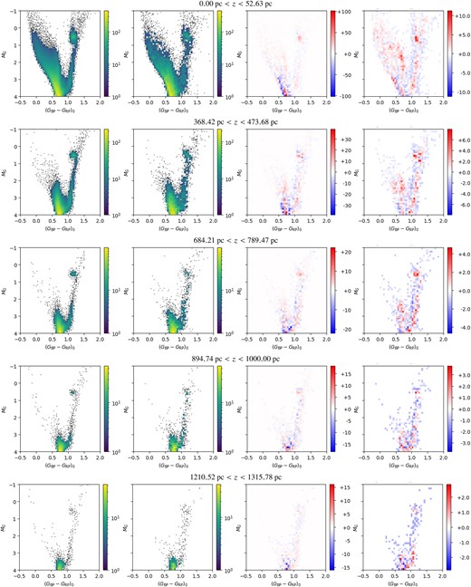
Comparison between the best-fit models and the observations in four slices of the sample, with distance from the Galactic plane increasing from the top panel to the bottom panel. For every row, from left to right, the Hess diagrams correspond to: the model M produced with the best fitting parameters, the observations O, the residuals M-O, and the significance (M-O)/|$\sqrt{\text{O}}$|.
The fitting method, we use also produces a number of young stars than is larger that expected, as highlighted by an upper main sequence more extended towards bright magnitudes in the best fit model than in the observations. While possible sources for this issue will be discussed in the following section, we note here that the uncertainty on this young component is considerable and its contribution to the total mass is minimal.
Before discussing the SFH, we comment briefly on the other fit parameters. First, we find only small offsets in the observed versus model photometric parameters, namely ΔMG = 0.04321 ± +0.0009 mag and Δ(GBP − GRP)0 = 0.01542 ± −0.0002 mag. These are reasonable given the known uncertainties in Gaia magnitudes and the difficulties in reproducing a new photometric system with synthetic photometry.9 Second, we find that Δ[Fe/H]1 = −0.0764 ± 0.0008 dex and Δ[Fe/H]16 = −0.083 ± 0.001 dex therefore the AMR is shifted to slightly smaller metallicities than in the reference AMR. Comparing our best fit AMR with the results of APOGEE and GALAH, shown in Fig. D1, we note that they are generally not in contrast. However, a detailed verification would require the addition of spectroscopic data, with its own selection function to be taken into account, in our SFH-recovery method. This kind of analysis will be pursued in a future work in this series.
Finally, we find a high initial binary fraction, more precisely fbin = 0.984 ± 0.003. For the moment, suffice it to recall that a similarly high fraction of binaries has also been suggested by the frequency of the ‘astrometric signals’ expected from binaries as compared to those observed in the Gaia sample of nearby stars (Penoyre, Belokurov & Evans 2022). On the other hand, the broadening of the lower main sequence in Gaia CAMD seems to suggest fbin values closer to 0.4 (Dal Tio et al. 2021). Both estimates strongly depend on the assumed intrinsic distribution of binary periods; however, there is a good agreement between the distributions assumed by the above-mentioned authors (based on Raghavan et al. 2010 and Moe & Di Stefano 2017, respectively). Therefore, the real fraction of binaries appears undefined at the moment, with different subsamples of Gaia data and methods providing different estimates. Fortunately, our main results for the SFH depend little on the final value of fbin. These aspects are discussed in more detail in Appendix E of the online supplementary material.
5 RESULTS AND DISCUSSION
Fig. 5 illustrates the main result of this paper, namely the SFR per unit volume in every slice and for all age bins. The information on the SFR is also presented in Table G2, together with the error bars. There are multiple ways in which this information can be interpreted.
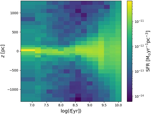
Plot of the SFR per unit volume, as determined for all slices and all age bins. It can be seen how the young stars are mostly concentrated on the Galactic plane while older ones are more dispersed.
5.1 The SFR as a function of height z
From Fig. 5, it is evident that the SFR strongly varies with z, and in a way which is almost symmetrical with respect to z = 0.
Fig. 6 presents the best-fit star formation rates (SFR) for the same slices as in Fig. 4. It can be appreciated that as we increase z from 0, the peak of SFR progressively moves towards older ages, and the overall SFR decreases.
![The SFR per unit volume as a function of age determined for the same slices of the sample shown in Fig. 4, also indicated on top of each panel. The blue lines represent the best fitting SFR values, while the grey-shaded areas and the dashed lines mark the 68 and 94 per cent confidence intervals, respectively. We note that the SFR at young ages (log (t[yr]) ≲ 7.5) is non-zero even at large z, although it is very uncertain.](https://oup.silverchair-cdn.com/oup/backfile/Content_public/Journal/mnras/527/1/10.1093_mnras_stad2952/2/m_stad2952fig6.jpeg?Expires=1750225619&Signature=eka9m6bJrQj~Pj4t-0Lmz4fZIwh~mb9z1hHlDvqmBxes1ywqOLtlwlsVpZvTGaZBpgZPB3EFOeoP99yQu-DwJBRWhGGHMaebwQVvp8jz9pzyRsuaoSxHz840giBvBGo5PFq0eelkfVRY-8UCnL-KOjQ8hW6vCCQkGzlpfE-jHmrS75sPyOJFlkYsfjonr0f67NbhrIf2df47jF05j1afN3l01O6tjeu55sQwe7FJr8Nf6L09Z4XIlU1~QPqcRARSb5xPaivBQlbJ-szE2E1JEqmyz78gJsVMjqIBVhxVKPnxD5Olr3YrsxA6nH25BumXRPBiLylTSNTrv5G-saL-Ow__&Key-Pair-Id=APKAIE5G5CRDK6RD3PGA)
The SFR per unit volume as a function of age determined for the same slices of the sample shown in Fig. 4, also indicated on top of each panel. The blue lines represent the best fitting SFR values, while the grey-shaded areas and the dashed lines mark the 68 and 94 per cent confidence intervals, respectively. We note that the SFR at young ages (log (t[yr]) ≲ 7.5) is non-zero even at large z, although it is very uncertain.
An important clarification is necessary at this point: our method determines the SFR where it is observed now, and not at their place of birth. With regard to the vertical distribution, it means that the old populations that are now observed at high |z| could have (and probably have) been born closer to the Galactic plane, and just got dispersed vertically as age increased (see next subsection). The same can be said with regard to the radial distribution in the Galaxy: older populations might have been born in different disc locations, and be observed now while in the solar neighbourhood (in a process commonly known as radial migration, see Lu et al. 2022 and references therein). This uncertainty about the place of birth of stellar populations is common to all SFH determinations in nearby galaxies.
We can qualitatively compare our results close to the Galactic plane with the results obtained by Dal Tio et al. (2021) for a Gaia DR2 sample within 200 pc of the Sun and excluding low galactic latitudes. For this comparison, we simply integrate the SFR obtained for all slices with |z| < 250 pc. We find the same peak of SFR in the log (t[yr]) = 9.3–9.5 age bin; however, we do not recover the peaks that they found at other ages. The differences do not appear substantial, and might be attributed to the different samples and methods, and the better understanding of the Gaia errors in DR3.
We can compare in the same way our results to those obtained by Alzate et al. (2021) for a sample of Gaia DR2 photometry within 100 pc from the Sun, by adding our best fitting SFR for slices with |z| < 105 pc. A comparison is not straightforward: their results are presented using the relative weight aAGE, i of each isochrone; we do not have enough age resolution to compare the results of the oldest SFR down to t = 4.8 Gyr, and they refer to slightly different galactocentric radii. Nevertheless, in both cases, the SFR appears to be declining from this age down to t ≈ 0.1 Gyr, the limit of their age interval. Finally, we find a peak in SFR at t ≈ 3 Gyr that is not found in their results.
5.2 The scale height as a function of age
From the best fitting SFRs of each slice, we can compute the scale height of the disc at every age bin, hz(t), by fitting the expected profile of the disc for the SFRs. In general, two functions have been used to describe this profile: the classical exponential
which applies well to stars at large heights (e.g. Gilmore & Reid 1983; Jurić et al. 2008), and the square hyperbolic secant
which should apply to a single-component, isothermal disc (Spitzer 1942; Bahcall 1984). None of these functions should be strictly valid in the case of a multicomponent disc as the MW one (see e.g. Sarkar & Jog 2020); however, they are still useful approximations, valid at high |z|, and they allow an easy comparison with previous results in the literature. We note that we have also introduced a constant c in both equations, which is usually absent.
We use both functional forms to fit the trend of SFR with |z| and examples of these fits performed in different ages bins are presented in Fig. 7. This figure clearly illustrates the difficulty in selecting a single functional form to describe the SFR profile with |z| at all ages. While achieving the optimal model selection is not in the scope of this work, it can be appreciated how the result in the 9.1 < log (t[yr]) < 9.3 age bin appears to be better fitted by the squared hyperbolic secant, at least for |z| < 600 pc, while the one in the 9.9 < log (t[yr]) < 10.1 bin appears to favour an exponential fit. Another aspect that becomes clear especially in the upper (younger) two panels is the need for the constant c in equations (10) and (11) for the younger ages, the lack of which would not allow a proper fit with either function of the flatter trend of the SFR at large |z|.
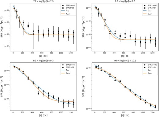
Fit of the SFR per unit volume (black circles and squares) with the exponential (blue) and squared hyperbolic secant (orange) functions.
The overall result of the SFR fits is summarized in Table 2 and in Fig. 8, and it clearly shows the tendency of hz to increase with age, irrespective of the functional form used. We note that there are two important details in this figure:
The scale heights for all young ages (t ≲ 500 Myr) are essentially constant with values smaller than 100 pc. However, the scale heights for the age bin with 7.7 < log (t[yr]) < 7.9 are notably higher, particularly in the youngest age bin.
For all ages smaller than 4 Gyr, the scale height appears to have an approximately linear trend with age. For the |$\operatorname{\operatorname{sech}^{2}}$| case, the hz flattens at values close to 450 pc for all older ages. For the exp case, some flattening occurs at later ages, but it is not so marked.
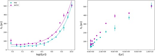
The scale height of the Galactic disc hz versus the mean age of every age bin. The cyan points are the exponential case, while the magenta points are for the case of the square hyperbolic secant. The left plot uses a logarithmic scale for the age, while the right one uses a linear one and shows that the linear trend in younger ages is lost at older ages, where the trend in hz flattens. The dashed lines in the left-hand panel show the results of the fits of equation (12).
| fexp | |$f_{\operatorname{\operatorname{sech}^{2}}}$| | ||||||||
|---|---|---|---|---|---|---|---|---|---|
| log (t1[yr]) | log (t2[yr]) | A | hz | c | χ2 | A | hz | c | χ2 |
| |$[10^{-11}\, \text{M}_\odot \, \mathrm{yr}^{-1}\mathrm{pc}^{-3}]$| | [pc] | |$[10^{-11}\, \text{M}_\odot \, \mathrm{yr}^{-1}\mathrm{pc}^{-3}]$| | |$[10^{-11}\, \text{M}_\odot \, \mathrm{yr}^{-1}\mathrm{pc}^{-3}]$| | [pc] | |$[10^{-11}\, \text{M}_\odot \, \mathrm{yr}^{-1}\mathrm{pc}^{-3}]$| | ||||
| 6.60 | 7.10 | 1.695 ± 0.674 | 76.7 ± 15.6 | 0.02605 ± 0.00462 | 25.8 | 1.178 ± 0.445 | 106.9 ± 19.2 | 0.26945 ± 0.00465 | 27.1 |
| 7.10 | 7.30 | 3.860 ± 1.244 | 46.8 ± 8.6 | 0.04999 ± 0.00531 | 13.3 | 2.858 ± 0.816 | 60.3 ± 9.8 | 0.50915 ± 0.00539 | 14.0 |
| 7.30 | 7.50 | 2.797 ± 1.149 | 36.2 ± 6.6 | 0.03326 ± 0.00292 | 12.8 | 1.497 ± 0.569 | 58.2 ± 9.0 | 0.33437 ± 0.00292 | 13.0 |
| 7.50 | 7.70 | 3.040 ± 1.215 | 40.1 ± 6.3 | 0.01333 ± 0.00218 | 19.7 | 1.798 ± 0.611 | 63.4 ± 7.6 | 0.13443 ± 0.00212 | 18.7 |
| 7.70 | 7.90 | 2.637 ± 0.743 | 46.3 ± 5.3 | 0.00899 ± 0.00099 | 11.4 | 1.507 ± 0.409 | 73.7 ± 7.6 | 0.00906 ± 0.00101 | 11.9 |
| 7.90 | 8.10 | 1.769 ± 0.565 | 41.8 ± 5.3 | 0.00784 ± 0.00119 | 28.6 | 1.071 ± 0.275 | 70.3 ± 6.6 | 0.00788 ± 0.00111 | 25.0 |
| 8.10 | 8.30 | 2.245 ± 0.704 | 43.9 ± 6.1 | 0.00513 ± 0.00078 | 33.7 | 1.427 ± 0.374 | 68.4 ± 7.2 | 0.00516 ± 0.00075 | 31.1 |
| 8.30 | 8.50 | 1.590 ± 0.221 | 70.9 ± 4.9 | 0.00383 ± 0.00055 | 20.9 | 1.043 ± 0.144 | 104.8 ± 6.9 | 0.00402 ± 0.00057 | 22.9 |
| 8.50 | 8.70 | 2.822 ± 0.657 | 55.3 ± 7.7 | 0.00226 ± 0.00113 | 176.4 | 2.018 ± 0.401 | 76.1 ± 8.4 | 0.00234 ± 0.00113 | 175.0 |
| 8.70 | 8.90 | 2.625 ± 0.203 | 90.7 ± 4.7 | 0.00270 ± 0.00074 | 72.2 | 1.816 ± 0.134 | 129.2 ± 6.0 | 0.00297 ± 0.00075 | 75.1 |
| 8.90 | 9.10 | 2.804 ± 0.143 | 120.0 ± 4.4 | 0.00315 ± 0.00108 | 80.9 | 1.974 ± 0.090 | 167.0 ± 5.1 | 0.00412 ± 0.00099 | 71.9 |
| 9.10 | 9.30 | 2.625 ± 0.147 | 145.8 ± 6.3 | 0.00382 ± 0.00222 | 179.6 | 1.862 ± 0.064 | 204.0 ± 5.0 | 0.00655 ± 0.00135 | 76.6 |
| 9.30 | 9.50 | 2.972 ± 0.196 | 211.1 ± 12.8 | 0.00000 ± 0.00653 | 573.8 | 2.096 ± 0.053 | 307.1 ± 6.0 | 0.00163 ± 0.00218 | 102.3 |
| 9.50 | 9.70 | 1.230 ± 0.135 | 252.2 ± 33.5 | 0.00000 ± 0.00814 | 396.6 | 0.865 ± 0.048 | 392.4 ± 20.4 | 0.00000 ± 0.00360 | 138.3 |
| 9.70 | 9.90 | 1.170 ± 0.040 | 373.7 ± 23.0 | 0.00000 ± 0.01244 | 92.1 | 0.890 ± 0.021 | 424.0 ± 11.1 | 0.03903 ± 0.00494 | 48.7 |
| 9.90 | 10.10 | 1.210 ± 0.027 | 512.0 ± 32.6 | 0.00000 ± 0.02142 | 104.8 | 0.896 ± 0.023 | 503.7 ± 17.3 | 0.09480 ± 0.01016 | 125.9 |
We remark that the constant c has been introduced in our fits because it improves a lot the fitting of both equations, especially in the case of young age bins. As can be seen in Table 2, it becomes completely irrelevant (i.e. compatible with a c = 0 value) for all ages |$\log t[\mathrm{yr}] > 8.5$| in both the exponential case and the |$\operatorname{\operatorname{sech}^{2}}$| cases, with the exception of the |$\operatorname{\operatorname{sech}^{2}}$| fit at the two oldest ages. For young ages, instead, the value of this constant is sizeable, but does not exceed 1.5 per cent in the former and 2.1 per cent in the latter of the value of the constant A, that is the value of the functions at z = 0. This constant is needed because, at all young ages, there is always a ‘background’ of star formation being detected at all z, even very far from the Galactic plane (see Figs 6 and 4). This background does not disappear with simple changes in the fitting method (see Appendix F of the online supplementary material). At least partially, it reflects the presence of real star counts along the bright main sequence at all z, as can be appreciated by the stars with MG < 2 and (GBP − GRP)0 < 0.5 in the observations of Fig. 4. It is not evident whether these main sequence stars are truly young. They could also be blue stragglers, which our binary models predict but maybe not in the right numbers to fit the observations, hence leading to the fitting of those stars by means of a young star formation. To clarify this feature, we need to first examine in detail the predictions of the binary BinaPSE module by means of special samples, which is not straightforward, and is not among the aims of this paper.
It should be noted at this point that this kind of determination of the scale height hz with high age resolution is currently possible only for the case of the MW. For external galaxies, there are alternative opportunities, given the availability of kinematics (see e.g. Dorman et al. 2015) and methods based on the dust geometry in inclined discs (e.g. Dalcanton et al. 2023). However, the age resolution attainable in such cases is quite limited.
Finally, we attempt to derive a fitting formula for the relation between hz and age, using the function
(equation (26) of Villumsen 1983), where hz, 0 is the scale height at t = 0, τ is a time-scale for the evolution of hz, and n controls the steepness of the relation. Fitting the values of hz in Table 2, we find
for equation (10) and
for equation (11), and the left-hand panel of Fig. 8 shows the two fits as dashed lines. Our best fitting n in the first case is remarkably close to the value of 2/3 favoured by Rana & Basu [1992, equation (4)], but the best fitting τ is about half of their value; the second case has a value of n closer to 1/2, and an even smaller τ.
We note that equation (12) is based on a simple model for the scattering of disc stars by giant molecular clouds (Villumsen 1983), and subsequent fits of the increase in velocity dispersion with age in their simulations (Villumsen 1985; Rana & Basu 1992). This model cannot be considered as a reference in modern times, given that it ignores important dynamical processes such as radial migration (Schönrich & Binney 2009) and the early accretion of small galaxies in the Galactic disc (Helmi 2020). However, it is remarkable that the simple form of equation (12) is still useful to represent the actual measurements of hz, now derived independently from any kinematical model or data.
5.3 Comparison with scale heights derived from simple star counts
A traditional way of deriving structural parameters of the MW disc is to determine the star counts of a specific kind of star for which distances can be derived, and fit them as a function of distance with exponentials. The method provides robust numerical results when applied to abundant objects such as Red Clump (RC; Cabrera-Lavers et al. 2007) or main sequence stars (MS; Jurić et al. 2008; Bovy 2017; Ferguson, Gardner & Yanny 2017), but suffers from one major problem: as the objects that are abundant generally sample a quite large interval of stellar ages, only an age-averaged scale height can be derived. RC stars, for instance, span the entire age interval from 1.5 to 10 Gyr, with some concentration around the younger ages (Girardi 2016), while the lower MS ones evenly sample all ages larger than a few Myr.
With the Gaia catalogue, this problem can be circumvented, to some extent, by using stars along the subgiant branch (SGB), which separate reasonably well in age. In the following, we attempt to derive the vertical scale height of the disc at different ages using their star counts, for the sake of providing a useful comparison with the results we have obtained in Section 5.2.
We take advantage of PARSEC v1.2S solar-metallicity isochrones (Bressan et al. 2012) computed at ages 9.3 ≤ log (t[yr])) ≤ 10.3, with a step of 0.1 dex in log (t[yr]), then select all the observed stars between the SGB portions of two subsequent isochrones, as illustrated in Fig. 9. To compare with the results obtained without age resolution, we also select stars in two other regions of the CAMD, namely the upper MS (which includes stars with 7.6 ≲ log (t[yr]) ≲ 9.2) and the RC, using simple CAMD boxes. Table G1 shows the counts we derive for all slices and age ranges, and the fit for a single age interval on the SGB and for the two CAMD boxes is shown in Fig. 10. Finally, Table 3 summarizes the scale heights we obtain.
![Regions of the CAMD used to determine the star counts for the slice with −368.42 pc < z < −263.16 pc. The isochrones correspond to the SGB phase at different ages (black lines, from log (t[yr]) = 9.3 to log (t[yr]) = 10.1) and the coloured points between them are the sources we selected for each age interval. The dashed boxes instead select young MS (left, yellow points) and Red Clump (right, cyan points) stars.](https://oup.silverchair-cdn.com/oup/backfile/Content_public/Journal/mnras/527/1/10.1093_mnras_stad2952/2/m_stad2952fig9.jpeg?Expires=1750225619&Signature=wwZ~EHNO2PgnqQJJzqYvxLQDZGrm~DhZIygsfrjFwga5My403vJbiY8QhCGkK3YUpPAseZ~da0jQgwvsddJ3cJWvF7x2gxjUzCVvD3xYxgJafZVzLOkwtQTBAr7CzcYY22Unf54YrpG8dIBf4zURNpZPMpQAnhRYbmvvlbFr2SveBx2PX1YGgJ-VP8G-MGtp1iUIZYVb2etcjOgss9ZNo30P65Fz96ecgcd7I2UMNtjKf2~K0bgHMYY33JWJCCcf3xFH8PYoxeXeMy0QkbJW8EDBMSJcfGLWJgn~lWasAp7OBqi-K3CfQTBY7A37e7ZtqLIyROi~bqTPrpTkLRsDxA__&Key-Pair-Id=APKAIE5G5CRDK6RD3PGA)
Regions of the CAMD used to determine the star counts for the slice with −368.42 pc < z < −263.16 pc. The isochrones correspond to the SGB phase at different ages (black lines, from log (t[yr]) = 9.3 to log (t[yr]) = 10.1) and the coloured points between them are the sources we selected for each age interval. The dashed boxes instead select young MS (left, yellow points) and Red Clump (right, cyan points) stars.
![Star counts per unit volume from the data and their fits with the exp (blue lines) and $\operatorname{\operatorname{sech}^{2}}$ (orange lines) functions. The shape of the black markers indicate counts at z ≥ 0 (circles) and z < 0 (squares). Panels from the top to the bottom correspond to stars selected in three different regions illustrated in Fig. 9: SGB stars between the isochrones of log (t[yr]) = 9.4 and log (t[yr]) = 9.5, MS stars, and red clump stars, respectively.](https://oup.silverchair-cdn.com/oup/backfile/Content_public/Journal/mnras/527/1/10.1093_mnras_stad2952/2/m_stad2952fig10.jpeg?Expires=1750225619&Signature=n~SGcOqDMm56-V5cFndsGit6iSdZz11276MVdSOGeiZ3~12~-ZwSgt02vJezDMQRfaBD0p1DRG5D-qqKsIkX2UlEp0uut7KxxS6dEaxRopWaB37nJf~yeZFQGiFfRoMwZnvj9MM2IjECUQ2DYbS9nljyQlZNM4kVHZN-qCp0lzLyTMzASNeU1lZKJdYSrBCnW1p0uc6F9ydoyz5CiuiDIIU0VXF~fuLa5479Z5AeXbTh5lJEdZTB~Rn~~gZ4bUBUzjdr0HnoeshNA0M02RtDebbZol67w05O3VXf1E0Db2F7Oh-Y~BJiIi~or1P26M3dQcEbgFV4PdgWNfyVqZysAg__&Key-Pair-Id=APKAIE5G5CRDK6RD3PGA)
Star counts per unit volume from the data and their fits with the exp (blue lines) and |$\operatorname{\operatorname{sech}^{2}}$| (orange lines) functions. The shape of the black markers indicate counts at z ≥ 0 (circles) and z < 0 (squares). Panels from the top to the bottom correspond to stars selected in three different regions illustrated in Fig. 9: SGB stars between the isochrones of log (t[yr]) = 9.4 and log (t[yr]) = 9.5, MS stars, and red clump stars, respectively.
Best fit parameters for the exponential (hz, exp ) and squared hyperbolic secant (|$h_{z, \operatorname{\operatorname{sech}^{2}}}$|) fits. The first column specifies the region of the CAMD used: the first block of rows refers to star counts between isochrones with the given ages at the SGB phase (upper panel of Fig. 10), while the second block uses simple CAMD ‘boxes’ (middle and bottom panel of Fig. 10). The second and third columns in the case of the SGB show the ages of the two isochrones between which the star counts are computed.
| fexp | |$f_{\operatorname{\operatorname{sech}^{2}}}$| | |||||||||
|---|---|---|---|---|---|---|---|---|---|---|
| Phase | log (t1[yr]) | log (t2[yr]) | A | hz | c | χ2 | A | hz | c | χ2 |
| |$[10^{-5}\text{counts}\, \mathrm{pc}^{-3}]$| | [pc] | |$[10^{-5}\text{counts}\, \mathrm{pc}^{-3}]$| | |$[10^{-5}\text{counts}\, \mathrm{pc}^{-3}]$| | [pc] | |$[10^{-5}\text{counts}\, \mathrm{pc}^{-3}]$| | |||||
| SGB | 9.3 | 9.4 | 0.800 ± 0.062 | 211.4 ± 16.8 | 0.0080 ± 0.0048 | 25.4 | 0.577 ± 0.040 | 278.6 ± 16.1 | 0.0144 ± 0.0038 | 24.1 |
| 9.4 | 9.5 | 1.990 ± 0.123 | 264.2 ± 19.5 | 0.0015 ± 0.0146 | 52.5 | 1.461 ± 0.071 | 335.3 ± 14.5 | 0.0301 ± 0.0084 | 37.7 | |
| 9.5 | 9.6 | 5.009 ± 0.221 | 296.3 ± 16.8 | 0.0000 ± 0.0319 | 75.0 | 3.693 ± 0.104 | 376.8 ± 9.8 | 0.0685 ± 0.0148 | 36.2 | |
| 9.6 | 9.7 | 3.623 ± 0.154 | 318.7 ± 19.4 | 0.0000 ± 0.0283 | 53.3 | 2.646 ± 0.076 | 408.7 ± 11.7 | 0.0497 ± 0.0137 | 29.2 | |
| 9.7 | 9.8 | 3.378 ± 0.149 | 388.1 ± 31.6 | 0.0000 ± 0.0497 | 64.8 | 2.536 ± 0.078 | 463.3 ± 16.1 | 0.0832 ± 0.0217 | 35.5 | |
| 9.8 | 9.9 | 3.126 ± 0.107 | 445.3 ± 36.1 | 0.0000 ± 0.0585 | 39.8 | 2.352 ± 0.077 | 470.2 ± 19.2 | 0.1689 ± 0.0270 | 35.4 | |
| 9.9 | 10.0 | 3.096 ± 0.114 | 542.8 ± 63.6 | 0.0000 ± 0.1062 | 50.5 | 2.285 ± 0.090 | 576.5 ± 35.8 | 0.1804 ± 0.0566 | 57.5 | |
| 10.0 | 10.1 | 1.584 ± 0.116 | 367.7 ± 47.0 | 0.0000 ± 0.0320 | 77.0 | 1.109 ± 0.076 | 497.9 ± 41.9 | 0.0117 ± 0.0239 | 84.8 | |
| Upper main sequence | 22.892 ± 1.160 | 106.3 ± 4.0 | 0.0199 ± 0.0115 | 167.4 | 16.184 ± 0.882 | 147.0 ± 5.5 | 0.0314 ± 0.0127 | 219.5 | ||
| Red Clump | 10.890 ± 0.307 | 288.3 ± 10.2 | 0.0571 ± 0.0436 | 61.8 | 8.131 ± 0.257 | 347.0 ± 9.9 | 0.2639 ± 0.0341 | 87.6 | ||
Visual inspection shows that most fits are of good quality. In the case of SGB star counts, the resulting scale heights are compatible with the values derived from the SFR for the same age bins (Table 2 and Fig. 11), generally confirming our previous conclusions about the increase of hz with age. This appears to confirm the suitability of the simpler method based on counts of SGB stars. The same cannot be said for the scale heights derived from the CAMD boxes. Although the fitting of RC star counts is also excellent (bottom panel of Fig. 10), hz ∼ 300–350 pc clearly corresponds to an intermediate value, valid at ages of ∼3 Gyr, and cannot be assigned to the entire disc. Similarly, for the upper MS hz ∼ 100–150 pc appears to be more in line with the scale height of the older part (t ≳ 9 Gyr) of its age interval.
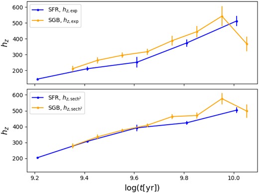
Comparison of hz obtained from the fits of the SFR and from the counts on the SGB, limited to the ages available in the latter case. Upper panel. Exponential fit. Lower panel. Squared hyperbolic secant fit.
More generally, we note that there is no single place in the CAMD that corresponds exactly to a single-burst stellar population, especially when we consider the populations of binaries, and the possibility of having a broad age-metallicity relation at old ages. As a result, scale heights derived from simple star counts will always be somewhat smeared out with respect to the true ones, even when referring to the SGB sections. Moreover, the SGB method does not apply to young ages.
Our method, based on the fitted SFR, represents an attempt to reduce these uncertainties. At the same time, it directly provides a quantitative measure of the total mass of stars involved in every fitted exponential or squared hyperbolic secant function therefore telling us how different discs compare in terms of total mass or surface density, as we discuss in the following subsection.
5.4 The vertically-integrated SFR
From the results, we get for each slice, we can compute the overall, vertically integrated SFR of the solar cylinder:
where Δzn = zmax − zmin. This function is presented in Fig. 12 and in Table 4. There appears to be an almost linearly decreasing surface SFR from the oldest ages up to the log (t[yr]) = 8.3–8.5 bin, broken in two phases by the peak in SFR at the log (t[yr]) = 9.3–9.5 bin. At bins younger than this one, the surface SFR appears to be somewhat constant down to the log (t[yr]) = 7.3–7.5 bin. The youngest age bins show an increase in SFR, but the large errors associated to these estimates prevent a definitive conclusion.
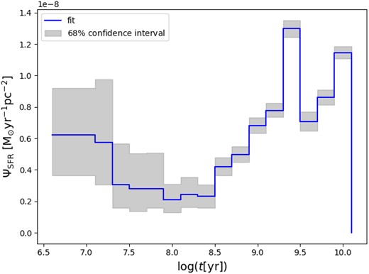
Overall surface SFR density of the solar cylinder at each age bin.
Total SFR per unit area for each age bin is computed in three different ways: by just adding the fitted SFR (third column) and integrating the exponential and square hyperbolic secant functions (fourth and fifth columns, respectively) betweenz |$z=-1315.78$| and 1315.78 pc.
| log (t1[yr]) | log (t2[yr]) | ΨSFR | |$\Psi _\mathrm{\exp }(t)$| | |$\Psi _\mathrm{\operatorname{\operatorname{sech}^{2}}}(t)$| |
|---|---|---|---|---|
| |$[10^{-9}\, \text{M}_\odot \, \mathrm{yr}^{-1}\mathrm{pc}^{-2}]$| | ||||
| 6.60 | 7.10 | |$6.20_{-2.60}^{+3.00}$| | 3.29 | 3.14 |
| 7.10 | 7.30 | |$5.70_{-2.70}^{+4.00}$| | 4.93 | 4.63 |
| 7.30 | 7.50 | |$3.10_{-1.50}^{+2.60}$| | 2.90 | 2.52 |
| 7.50 | 7.70 | |$2.80_{-1.40}^{+2.20}$| | 2.79 | 2.59 |
| 7.70 | 7.90 | |$2.80_{-1.20}^{+2.30}$| | 2.68 | 2.43 |
| 7.90 | 8.10 | |$2.11_{-0.82}^{+1.00}$| | 1.69 | 1.69 |
| 8.10 | 8.30 | |$2.44_{-0.83}^{+1.09}$| | 2.11 | 2.07 |
| 8.30 | 8.50 | |$2.31_{-0.72}^{+0.76}$| | 2.36 | 2.28 |
| 8.50 | 8.70 | |$4.21_{-0.54}^{+0.59}$| | 3.18 | 3.12 |
| 8.70 | 8.90 | |$4.97_{-0.47}^{+0.54}$| | 4.83 | 4.76 |
| 8.90 | 9.10 | |$6.81_{-0.47}^{+0.50}$| | 6.81 | 6.69 |
| 9.10 | 9.30 | |$7.79_{-0.43}^{+0.45}$| | 7.76 | 7.75 |
| 9.30 | 9.50 | |$12.99_{-0.54}^{+0.53}$| | 12.52 | 12.89 |
| 9.50 | 9.70 | |$7.09_{-0.59}^{+0.59}$| | 6.17 | 6.74 |
| 9.70 | 9.90 | |$8.60_{-0.48}^{+0.49}$| | 8.49 | 8.37 |
| 9.90 | 10.10 | |$11.47_{-0.38}^{+0.39}$| | 11.44 | 11.00 |
Similar quantities can be derived by integrating equations (10) and (11) from z = −1315.78 to 1315.78 pc, giving origin to the functions |$\Psi _\mathrm{\exp }(t)$| and |$\Psi _\mathrm{\operatorname{\operatorname{sech}^{2}}}(t)$|. Their values are reported in Table 4, together with ΨSFR(t). As can be noticed, the three estimates are very similar, except at very young ages. The benefit of defining these latter quantities is that they enable us to easily implement our current results in population synthesis codes like TRILEGAL (Girardi et al. 2005). As a result, we can perform more accurate simulations of the Galactic disc for various spatial samples and photometric systems.
Our vertically-integrated SFRs, Ψ(t), represent a volume large enough to allow comparisons with other SFRs present in the literature. For instance, Ruiz-Lara et al. (2022) modelled Gaia DR2 data for a sphere of radius 2 kpc centred on the Sun, finding three SFR peaks at ages 5.7, 1.9, and 1.0 Gyr. Direct comparisons with our results are not straightforward given the different age resolution adopted, but comparing their fig. 2 with our Fig. 12, we can see that the overall trend of SFR constantly decreasing with age is similar. However, they find a strong peak in SFR around 6 Gyr, while we find one in the younger 9.3 < log (t[yr]) < 9.5 age bin (ages from 2 to 3 Gyr). Concerning the other SFR peaks, we likely do not have a good enough age resolution to see them. Interestingly, the results might agree at the youngest ages (younger than 0.1 Gyr), where in both cases the SFR appears to have a boost.
Note that our 2–3 Gyr peak coincides with the one found by Mor et al. (2019), and might correspond to the 3 Gyr peak introduced by Sysoliatina & Just (2022). Both works are based on the modelling of the entire solar neighbourhood as sampled by Gaia.
5.5 The stellar mass formed in the solar cylinder
The contribution of each age bin to the total mass of stars ever produced is shown in Fig. 13. Similarly to Fig. 12, there is a decreasing amount of mass produced from the older to the younger ages, with a bump at the log (t[yr]) = 9.3–9.5 bin. Due to the increased SFR of the youngest ages, the trend appears to become constant for ages younger than the log (t[yr]) = 7.5–7.7 age bin. Nevertheless, the overall contribution of these young age bins to the total mass is minor compared to the other age bins.

1Total mass of stars produced in the solar cylinder in each age bin.
Summing together all contributions over the interval of age we explored, we determine the total mass of stars ever formed in the solar cylinder:
and the surface density of stars ever formed:
This quantity is of interest as it allows comparing our Galaxy with other disc galaxies for which the SFR cannot be investigated in the full 3D space, but their SFR density can be derived across the disc either by using resolved photometry from HST and JWST (e.g. Williams et al. 2017; Lazzarini et al. 2022), or integral field spectroscopy (e.g. García-Benito et al. 2017; López Fernández et al. 2018). In addition, from our results, we can also derive the contribution of each age bin to the surface SFR, which is shown in Table 2.
We recall that a fraction of the mass we derive has already been returned to the ISM, and may have been locked up again in successive generations of stars, in amounts that cannot be quantified unless we build complex chemical evolution models of the MW disc. Therefore, the surface density of equation (17) is not expected to coincide with the present mass density in the solar neighbourhood, which is usually derived with the help of the stellar kinematics. It is none the less comforting that the total mass density of stars ever formed has the same order of magnitude as the kinematically-derived one, which amounts to |$\Sigma _\mathrm{kin}(R_\odot) = 61\!-\!84\, \text{M}_\odot \, \mathrm{pc}^{-2}$| at heights of ∼1 kpc (e.g. Kuijken & Gilmore 1991; Holmberg & Flynn 2004; Bienaymé et al. 2014; Binney & Vasiliev 2023).
Moreover, we note that our estimates of ΣSFR and Mtot could still be reduced, systematically, by factors of about 40 to 60 per cent, if the binary fraction that characterizes our sample should turn out significantly smaller that the fitted value of fbin = 0.984. This aspect is discussed in Appendix E.
5.6 The apparent vertical metallicity gradient
One of our basic assumptions is that stellar populations in the solar cylinder follow a single and relatively narrow AMR. It is interesting to check whether this assumption is compatible with the observed vertical trends of stellar metallicities.
For instance, let us try to reproduce the metallicity gradient found by Imig et al. (2023) from the last release of the Apache Point Observatory Galactic Evolution Experiment (APOGEE) data. They have considered a high-quality subsample of APOGEE targets defined by |$1 < \log g[\text{cm}\, \text{s}^{-2}] < 2$|, 3500 < Teff/K < 5250. Stars with these characteristics are all red giants, but they do not cover a well-defined range in Gaia magnitudes and colours. Therefore, to derive the metallicity distribution for these stars, we build a new set of partial models comprising only the stars in these log g and Teff intervals, for exactly the same population parameters as in our previous analysis (see Section 3.1). We then use our best-fitting solution to derive numbers of expected APOGEE targets at every |z| and [Fe/H] bin, hence constructing the 2D histogram shown in Fig. 14. The blue line in the figure shows the linear fit to the mean [Fe/H] in each vertical slice:
and therefore the vertical metallicity gradient we obtain is |$-0.068\, \text{dex}\, \text{kpc}^{-1}$|. Additionally, for the entire solar cylinder, we find that the mean metallicity is [Fe/H] = −0.19.
![Counts per cubic parsec of giant stars at different |z| and [Fe/H], obtained from the best-fit solution, including the spread of 0.1 dex along the metallicity axis. The blue line represents the linear fit to the mean [Feh/] computed in each bin of |z|, with a slope of $-0.068\, \, \text{dex}\, \text{pc}^{-3}$.](https://oup.silverchair-cdn.com/oup/backfile/Content_public/Journal/mnras/527/1/10.1093_mnras_stad2952/2/m_stad2952fig14.jpeg?Expires=1750225620&Signature=b8p~PORnVdPdGmKArHIrVTWZ-r~6ktjYh5Gdl3xg9RjvDalSxcsX0mwhyHIOwIEQVWtbpQlMo~3ojT8~fs43jvLf5sFMQ~UBJoVJbeJ3VDtxv4JOJY04sRFit3Ou5yH9T8tG0glUztrL2ENduNtGBt~PIgg8LgY2QnLG-zWd4a4KU~gAJQ3X3fjFQtdGbnEh5xgahE2SmGVZQdSjtXHcyOP0otSbGZ-D1MH0nU1xr7t4ZwschxtYrTXANMUlPBHGix6g7HiFLfUUSHacm~sbzhi8Y8Fwj12shdhQrStSqUMTleHNVj25XxqHyg~0XnBneioREIfCtFOvgSAqInNhTA__&Key-Pair-Id=APKAIE5G5CRDK6RD3PGA)
Counts per cubic parsec of giant stars at different |z| and [Fe/H], obtained from the best-fit solution, including the spread of 0.1 dex along the metallicity axis. The blue line represents the linear fit to the mean [Feh/] computed in each bin of |z|, with a slope of |$-0.068\, \, \text{dex}\, \text{pc}^{-3}$|.
Although we infer a vertical metallicity gradient significantly smaller than the |$-0.315\pm 0.009\, \text{dex}\, \text{kpc}^{-1}$| mean value found by Imig et al. (2023) near the solar neighbourhood, this exercise demonstrates that a vertical metallicity gradient naturally comes out from the fitting of the SFH in the solar cylinder, even when a single AMR is assumed, as the result of the systematic increase in scale height of older (and metal poorer) populations.
Also, it is important to note that APOGEE does not sample all stars in the log g and Teff intervals selected for this test. The selection of APOGEE primary targets (Zasowski et al. 2013) is based mainly on 2MASS photometry, and it is limited by the apparent brightness of the available targets and by the finite number of observing nights and fibres in the APOGEE spectrograph. Moreover, APOGEE can clearly distinguish populations according to their [α/Fe], which is a capability still not implemented in our CMD fitting method. Therefore, our attempt to reproduce their metallicity gradient can only be approximated at the moment. Work is underway to fully implement APOGEE target selection in our method, in order not only to verify the abundance gradients derived by the method but also to actually use their metallicity information during the CMD fitting.
It is also worth mentioning that slightly smaller values for the vertical metallicity gradient have been found with different surveys, for instance Önal Taş et al. (2016) find |$-0.157\pm 0.003\, \text{dex}\, \text{kpc}^{-1}$| from red clump stars within |z| < 3 kpc in RAVE, Duong et al. (2018) finds |$-0.18\pm 0.01\, \text{dex}\, \text{kpc}^{-1}$| from thin disc stars (low-α) in GALAH, Hawkins (2023) finds |$-0.15\pm 0.01\, \text{dex}\, \text{kpc}^{-1}$| using OBAF stars from LAMOST.
6 SPATIALLY-CORRELATED SFHS
The present results, illustrated in Fig. 5, tell of a SFH that, despite being characterized by some noise, is strongly correlated among different locations in the solar cylinder, especially at old ages. The spatial correlation occurs at lengths that are comparable to the scale heights we have discussed in Section 5.2. It also has a very simple interpretation: the stellar populations we see in different slices are partially the same, and even more so at old ages.
Can this simple observation be used to improve the derivation of the SFHs, perhaps allowing us to reduce the noise that characterizes the SFH maps of Fig. 5? To answer this question, we developed the alternative formalism that is described here.
6.1 Adopting a spatial correlation: the method
To include a term for the spatial correlation of the solutions at different z, we do not need to heavily change our method. In particular, we can add a term to the likelihood that accounts for the correlation of the SFRs, favouring more correlated solutions. We take inspiration from Gaussian processes, and we build a correlation matrix |$\boldsymbol {\mathsf {R}}$| whose entries are defined by an exponential kernel
where |$\boldsymbol {\mathit {x}}_n$| and |$\boldsymbol {\mathit {x}}_m$| are vectors of coordinates identifying the centre of two slices, and li is the correlation length.
The subscript i marks the dependence on age of the correlation length; in fact, we assume that each age bin has a different value and that it should be increasing with age. In other words, we are assuming that, from their birth, stellar populations have travelled and got gradually mixed (or spatially distributed) over a distance of the order of the correlation length. Importantly, it should be noted that we do not attempt to derive the correlation lengths li, but we adopt the results we get from the exponential fit of the SFR presented above (hz, exp in Table 2). Finally, we compute the covariance matrix for each age bin as
where σn and σm are the noise standard deviations for the slice n and m.
The likelihood in equation (8) is updated to the following:
where |$\boldsymbol {\mathit {a}}$| is the vector containing the SFR of all slices and |$\log \mathcal {L}_{\mathrm{corr}}(\boldsymbol {\mathit {a}}_{0},\pmb {\Sigma };\boldsymbol {\mathit {a}})$| is the log-likelihood of the correlated |$\boldsymbol {\mathit {a}}$|, that is the log-likelihood of a multivariate normal distribution centred on |$\boldsymbol {\mathit {a}}_{0}$| and having covariance matrix |$\pmb {\Sigma }$|.
6.2 Adopting a spatial correlation: the results
The result of adding the correlation term to our analysis is presented in Fig. 15. Comparing this result to Fig. 5, it is possible to appreciate that, while it maintains unchanged the overall trend, it shows a smoother distribution of SFR in the slices closer to the Galactic plane at all ages, and does not show any more the SFR peak at the youngest age in the slice just above the Galactic plane. Furthermore, the distribution of SFR appears to be more symmetric with respect to the Plane. This is presented in Fig. 16, which shows the difference between the SFR above and below the plane in the uncorrelated and correlated cases for three groups of slices: 0.0 < |z| < 250.0 (top panel), 250.0 < |z| < 700.0 (middle panel), 700.0 < |z| < 1350.0 (bottom panel). In all three panels, the values of SFR(z > 0) − SFR(z < 0) in the correlated case appear to be compatible with those of the uncorrelated one and they are also generally closer to zero, thus showing a more symmetric picture of the Disc. In addition, the correlated solution, due to the smaller 1σ uncertainties, can be considered more reliable than the uncorrelated one.
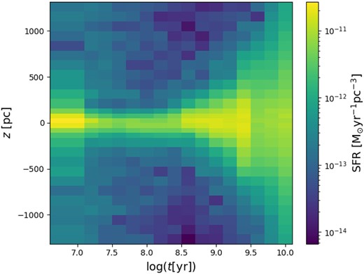
Plot of the SFR per unit volume, as determined for all slices and all age bins in the correlated case.
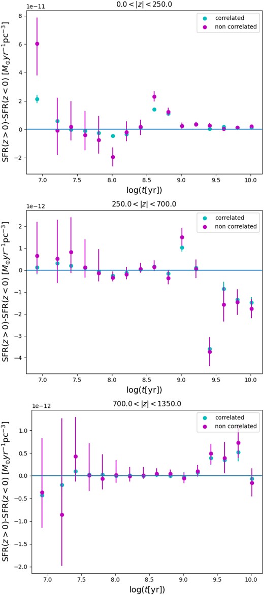
Difference between the fitted star formation rate above (z > 0) and below (z < 0) the Galactic plane in the uncorrelated (magenta points) and correlated (cyan points) for three groups of slices: 0.0 < z < 250.0 (top panel), 250.0 < z < 700.0 (middle panel), 700.0 < z < 1350.0 (bottom panel).
Fig. 17 shows the fits of the SFR at different age bins with equations (10) and (11). The differences with the uncorrelated case are not extreme, but it can be appreciated that the spread of the SFR at each age has decreased.
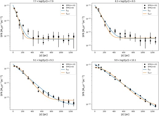
Fit of the SFR per unit volume (black circles and squares) with the exponential (blue) and squared hyperbolic secant (orange) functions in the case with correlation.
Looking at the values of hz, in Fig. 18, the general trend is the same, but the value of hz at the fifth age bin (7.7 < log (t[yr]) < 7.8) has decreased considerably and is now more in line with the ones found at the young ages. With regard to equation (12), in this case we obtain
for equation (10) and
for equation (11), and the left-hand panel of Fig. 18 shows the two fits as dashed lines. Comparing Fig. 8 with Fig. 18, it can be appreciated that the results in the case including the correlation have smaller fit residuals compared to the non-correlated ones.
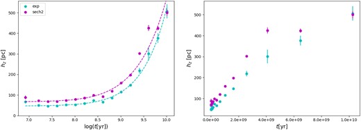
The scale height of the Galactic disc hz versus the mean age of every age bin in the case with correlation. The cyan points are the exponential case, while the magenta points are for the case of the square hyperbolic secant. The left plot uses a logarithmic scale for the age, while the right one uses a linear one and shows that, just as in the case without correlation, the linear trend in younger ages is lost at older ages, where the trend in hz flattens.
As a concluding remark, it should be noted that we have also implicitly adopted a perfect correlation between different slices, in the form of imposing that Δ(GBP − GRP)0, ΔMG, Δ[Fe/H], and fbin values are the same in all slices, which is already an improvement over current methods, while we use the flexible correlation on the ai coefficients. This is due to the assumption that populations seen at different z are the superposition of the same building blocks. A full correlated treatment could be implemented by applying the same kind of correlation to all parameters involved.
Overall, the changes brought by the correlation are not extreme and are compatible with the non-correlated one, but at the same time, the overall picture improves. The approach that we develop and apply for the first time in this work can be extended to other targets, and most importantly, to other galaxies, as long as enough photometric data and extensive ASTs are available.
7 CONCLUSIONS
In this work, we perform a simultaneous analysis of the SFH across several slices of a cylinder 2.6 kpc high and with a 200 pc radius centred on the Galactic plane close to the Sun. Our method is based on the fitting of the star counts across the CAMD obtained from Gaia data, a method routinely used in external galaxies with high-precision photometry. Just a few adaptations were needed in order to face the complexities of Gaia data; in particular, we introduce a more careful approach to dealing with binary systems and their resolvability into two components as a function of distance and do our best to simulate the incompleteness, parallax, and photometric errors present in Gaia data. Model parameters that should be common to all slices, such as the possible systematic shifts in colour and magnitude, the initial binary fraction, and the AMR, are all adjusted at the same time. Among our most relevant findings, we highlight the following aspects:
We derive the spatial density of SFR as function of both age and height from the Galactic plane.
Our results provide an improved picture of the SFH with respect to previous SFH papers based on Gaia. In particular, we clearly see the spatial dependence of the SFH with the height z above/below the Galactic plane.
Our space-resolved SFHs also allow us to quantify the increase in scale height with age in a way that was not possible before: using the entire section of the CAMD, which is sensitive to age, instead of just a few selected stellar tracers. A better resolution in age is expected with this method. We confirm that fitting star counts across the SGB section of the CAMD generally produces similar results for the scale height at ages larger than 2 Gyr. However, the same does not happen with the red clump, which just provides an age-averaged value of scale height.
Some details of the results are weird, as for instance the persistent low-level SFR at young ages and very far from the Galactic plane, which is indicated by a non-negligible value of the constant c in our fits of the scale height. These probably indicate shortcomings in stellar models and/or of Gaia data. Identifying these problems (rather than hiding them) is a necessary step to further improve the description of nearby stellar populations in the post-Gaia era.
The surface density of stellar formation as a function of age, Ψ(t), is derived in three different ways. These functions clearly reveal a period of enhanced star formation in the age bin going from 2 to 3 Gyr. This peak has some correspondence with peaks inferred by other authors at similar ages (Mor et al. 2019; Ruiz-Lara et al. 2022; Sysoliatina & Just 2022) but using different methods and data. Other peaks detected by these authors, however, do not appear in our results.
The total mass of stars formed per unit area, which we determine is roughly double that determined by studies using kinematic information within 1 kpc from the Galactic plane. This might be implying a high degree of matter recycling in successive generation of stars.
The parameters derived from our analysis, comprising Ψ(t), hz(t), [Fe/H](t), and fbin, can be easily implemented in our population synthesis code TRILEGAL (Girardi et al. 2005), hence allowing us to perform better simulations of the Galactic disc for different spatial samples and in other photometric systems. Indeed, a web interface incorporating these results10 is presently in preparation.
Finally, we modify the SFH-recovery method to take advantage of the very evident spatial correlation in the old SFH revealed by our analysis. An age-dependent correlation length is introduced along with its corresponding covariance matrix and changes in the computation of the model-data likelihood. The modified method is shown to provide less noisy and more symmetric SFH results with respect to the Galactic plane. We consider it as a promising way to improve SFH-recovery methods to be applied to nearby galaxies.
This work represents an intermediate step within a more ambitious project to improve the tools for the modelling and the interpretation of stellar populations in disc galaxies. The next steps of this project will include: a recalibration of the parameters defining the populations of binaries, the exploration of a large range in the Galactocentic radius, and the inclusion of spectroscopic and asteroseismic information into our modelling.
ACKNOWLEDGEMENTS
We thank the anonymous referee for the useful report. Alessandro Mazzi acknowledges financial support from Padova University, Department of Physics, and Astronomy Research Project 2021 (Progetti di Ricerca Dipartimentali 2021), and thanks the Center for Computational Astrophysics for the kind hospitality in New York. Léo Girardi acknowledges partial funding by an INAF Theory Grant 2022. Andrea Miglio acknowledges support from the ERC Consolidator Grant funding scheme (project ASTEROCHRONOMETRY, G.A. n. 772293 http://www.asterochronometry.eu). The Flatiron Institute is funded by the Simons Foundation.
We are grateful to the entire GaiaUnlimited team for their software and for organising this very helpful workshop.
This work has made use of data from the European Space Agency (ESA) mission Gaia (https://www.cosmos.esa.int/gaia), processed by the Gaia Data Processing and Analysis Consortium (DPAC, https://www.cosmos.esa.int/web/gaia/dpac/consortium). Funding for the DPAC has been provided by national institutions, in particular the institutions participating in the Gaia Multilateral Agreement.
DATA AVAILABILITY
The data underlying this article were accessed from the ESA Gaia archive (https://gea.esac.esa.int/archive/). The best-fitting models generated in this research will be shared on reasonable request to the corresponding author.
Footnotes
We use the python package from https://gitlab.com/icc-ub/public/gaiadr3_zeropoint
We denote here ‘spatial resolution’ the correlation length used by the authors to compute the map.
This is a subtle density bias closely related to the better-known Lutz–Kelker bias (Lutz & Kelker 1973) in the mean parallaxes.
Gaia’s detection efficiency drops for stars brighter than G ≈ 3 (Fabricius et al. 2021). A star with absolute magnitude MG = 0 has G = 3 at a distance d ≈ 40 pc, which means stars at this absolute magnitude inside a sphere of radius 40 pc are subject to saturation. The volume of this region is approximately 2.1 per cent of the volume of the slice. For MG = −1, d ≈ 63 pc, and the volume is 8.3 per cent of the slice’s volume. These values look, overall, compatible with the ≈5 per cent loss in stars observed in Fig. 3 for the slice closest to the Plane.
Although, as described in the following Section 4, the algorithm we use for the fit should not be affected significantly by local maxima.
These difficulties are made evident in the ‘standardization’ process adopted from Gaia Collaboration et al. (2022, see their fig. 4), who modify the transmission curves of well-established photometric systems to make the synthetic photometry of Gaia BP and RP spectra to reproduce the magnitudes of standard stars.
