


ABSTRACT
We report the first extensive optical flux and spectral variability study of the TeV blazar TXS 0506 + 056 on intranight to long-term time-scales using BVRI data collected over 220 nights between 2017 January 21 to 2022 April 9 using eight optical ground-based telescopes. In our search for intraday variability (IDV), we have employed two statistical analysis techniques, the nested ANOVA test and the power enhanced F-test. We found the source was variable in 8 nights out of 35 in the R-band and in 2 of 14 in the V-band yielding duty cycles (DC) of 22.8 per cent and 14.3 per cent, respectively. Clear colour variation in V − R was seen in only 1 out of 14 observing nights, but no IDV was found in the more limited B, I, and B − I data. During our monitoring period the source showed a 1.18 mag variation in the R-band and similar variations are clearly seen at all optical wavelengths. We extracted the optical (BVRI) SEDs of the blazar for 44 nights when observations were carried out in all four of those wavebands. The mean spectral index (α) was determined to be 0.897 ± 0.171.
1 INTRODUCTION
Blazars are active galactic nuclei (AGNs) characterized by highly collimated relativistic jets with half opening angles ≲ 5° closely aligned with the observer’s line of sight (e.g. Urry & Padovani 1995). The Doppler enhanced intense non-thermal radiation from this jet dominates the spectral energy distribution (SED) from radio to very high energy (VHE) γ-ray energies. Blazars are usually considered to be comprised of BL Lacertae (BL Lac) objects that show featureless spectra or very weak emission lines (equivalent width EW |$\le 5\,$|Å) (Stocke et al. 1991; Marcha et al. 1996), and flat-spectrum radio quasars (FSRQs) with prominent emission lines in their composite optical/UV spectra (Blandford & Rees 1978; Ghisellini et al. 1997). Blazars show flux and spectral variability across the entire electromagnetic (EM) spectrum, emit predominantly non-thermal radiation showing strong polarization (|$\gt 3{{\ \rm per\ cent}}$|) from radio to optical frequencies, and usually have core dominated radio structures.
The multiwavelength SEDs of blazars in log(νFν) versus log(ν) representation show double-humped structures in which the low-energy hump peaks in infrared (IR) through X-ray bands while the high-energy hump peaks at γ-ray energies (Fossati et al. 1998). The location of SED peaks are often used to classify blazars into two subclasses, namely LBLs (low-energy-peaked blazars) and HBLs (high-energy-peaked blazars). In LBLs, the first hump peaks in IR to optical bands and the second in GeV γ-ray energies (Padovani & Giommi 1995). Whereas in HBLs, the first hump peaks in UV to X-ray bands and the second in up to TeV γ-ray energies (Padovani & Giommi 1995). The emission of the lower energy SED hump is due to synchrotron radiation that originates from relativistic electrons in the jet. The high-energy hump can be attributed to two mechanisms. One of these is inverse Compton scattering of low-energy photons by the same electrons responsible for the synchrotron emission (synchrotron-self Compton) or external photons (external Compton), collectively known as the leptonic model (e.g. Böttcher 2007). The other mechanism is emission from relativistic protons or muon synchrotron radiation, referred to as the hadronic model (e.g. Mücke et al. 2003).
Flux variability over a wide range of time-scales is one of the definitional properties of blazars. On the basis of the time-scales over which it is observed, blazar variability can be divided into three somewhat arbitrary categories: microvariability (Miller, Carini & Goodrich 1989) or intraday variability (IDV; Wagner & Witzel 1995) or intranight variability (Gopal-Krishna, Sagar & Wiita 1993) (occurring on a time-scale of a few minutes to less than a day); short-term variability (STV; taking place on a time-scale of days to months); and long-term variability (LTV; over a time-scale of several months to years or even decades) (Gupta et al. 2004).
Colour–magnitude diagrams (CMDs) for blazars can be analysed to find any colour trends accompanying brightness changes. Three types of CMD behaviour could be discerned: redder-when-brighter (RWB), bluer-when-brighter (BWB), and achromatic. FSRQs mostly show RWB chromatism because the contribution of the accretion disc to the total emission is significant (Gu et al. 2006; Gaur et al. 2012c). The BWB behaviour seen in many BL Lacs is thought to arise from processes occurring in the relativistic jet, such as particle acceleration and cooling in the framework of the shock-in-jet model (e.g. Marscher & Gear 1985; Kirk, Rieger & Mastichiadis 1998). Alternatively, the BWB chromatism could arise from a Doppler factor variation on a convex spectrum (e.g. Villata et al. 2004b; Papadakis, Villata & Raiteri 2007). Finally, achromatic behaviour is frequently interpreted as being due to the variations of the Doppler factor, which are most likely explained in a framework involving changes in the viewing angle to the dominant emission region (e.g. Villata et al. 2002; Gu et al. 2006; Gaur et al. 2012c; Agarwal & Gupta 2015; Agarwal et al. 2016).
TXS 0506 + 056 is registered as a blazar in the Texas Survey of Radio Sources catalogue (Douglas et al. 1996). The first detection of a high-energy neutrino event from a blazar was reported from TXS 0506 + 056 on 2017 September 22 by the IceCube collaboration and was coincident in direction and time with a γ-ray flare (IceCube Collaboration et al. 2018a). Prompted by this discovery, an investigation was carried out of 9.5 yr of IceCube neutrino observations to search for excess emission at the position of the blazar, and an excess of high-energy neutrino events between 2014 September and 2015 March at energies around 290 TeV at a |$3.5\, \sigma$| level was indeed detected (IceCube Collaboration et al. 2018b). This object is the highest energy γ-ray-emitting blazar among those detected by the Energetic Gamma-Ray Experiment Telescope (EGRET) satellite in the γ-ray energy range (30 MeV−30 GeV) (Dingus & Bertsch 2001). It is identified as a jet-dominated in the low-hard state during neutrino flaring in 2014/2015, and so provides evidence for the blazar jet acting as an accelerator of cosmic-ray particles which produce neutrinos (Padovani et al. 2018). TXS 0506 + 056 was independently detected at high-energy γ-rays with the Large Area Telescope (LAT) onboard the Fermi satellite (Tanaka, Buson & Kocevski 2017), the MAGIC telescope (Ansoldi et al. 2018), and the AGILE γ-ray telescope (Lucarelli et al. 2019), which strengthens the case for TXS 0506 + 056 being a VHE γ-rays emitting BL Lac as well as a neutrino emitting source. However, Padovani et al. (2019) claimed that TXS 0506 + 056 is a masquerading BL Lac, i.e. a FSRQ with hidden broad lines and a standard accretion disc that is outshined by the jet emission. During the intensive follow-up observations, the redshift of TXS 0506 + 056 was successfully determined to be z = 0.3365 (Paiano et al. 2018). The analysis of single-dish 15 GHz radio flux densities from the Owens Valley Radio Observatory (OVRO) spanning between 2008 and 2018 indicates that the core of TXS 0506 + 056 is in a highly flaring state coincident with the neutrino event 170922A (Britzen et al. 2019; Kun, Biermann & Gergely 2019). In this paper, we are reporting an extensive optical variability study of the first neutrino emitting TeV blazar TXS 0506 + 056 on diverse time-scales.
This paper is organized as follows: Section 2 provides an overview of the telescopes, photometric observations, and the data reduction procedure. Analysis techniques we used to search for flux variability and correlations between bands are discussed in Section 3. Results of our study are reported in Section 4. A discussion and conclusions are provided in Section 5.
2 OBSERVATIONS AND DATA REDUCTION
Optical photometric observations of the TeV blazar TXS 0506 + 056 were carried out using eight ground-based telescopes. Two telescopes are located in India: the 1.04 m Sampurnanand Telescope (ST), and the 1.3 m Devasthal Fast Optical Telescope (DFOT), ARIES, Nainital. Both of these telescopes are equipped with CCD detectors and broad-band Johnson UBV and Cousins RI filters. The source was observed with alternate observations in the V and R bands for a total of 37 nights between 2019 November 7 and 2021 January 31. One or two B and I image frames were also taken on each night of observations.
Observations of this source with the 60 cm Cassegrain telescope located at the Astronomical Observatory Belogradchik, Bulgaria, were carried out over the course of 40 nights from 10 October 2018 to 17 August 2020, consisting on a single optical frame in B, V, R, and I bands each night. These 40 nights of observations were presented in Bachev et al. (2021). The 2-m Ritchey–Chretien telescope at the National Astronomical Observatory Rozhen, Bulgaria, observed only a single night in V, R, and I bands on 17 August 2020. Observations of the source with the 1.3 m modified RC telescope at Skinakas Observatory, Crete, Greece were taken during six nights, 2019 August 26–31 in the optical B, V, R, and I bands.
Three additional nights of observations were taken with the 0.6 m Helen Sawyer Hogg (HSH) telescope at CASLEO, Argentina (on loan from the University of Toronto, Canada) in B, V, R, and I bands. Additional V-band observations from AAVSO1 (American Association of Variable Star Observers) were carried out from amateur astronomers’ two telescopes in Spain and Italy.
The technical parameters and instrumental details are summarized in Table 1. A total of 220 nights of optical photometric observations of TXS 0506 + 056 were carried out between 2017 January 21 and 2022 April 9. The AAVSO data are included, with most of these observations being done in the V and R bands. In 35 nights, the observation duration is ≥1 h, which we use to study IDV behaviour of the blazar. R-band observations were carried out in each of them but they were performed in the B, V, and I bands in only some of the nights. Considering these 35 nights of observations, we obtained data for 35, 14, 7, and 6 nights, respectively, to look for IDV in the R, V, I, and B bands. During 44 nights, we have at least 1 frame in all four optical bands, which are useful for studying this portion of the SED. The observation log is provided in Table 2.
Details of telescopes and instruments used.
| A1 | A2 | B | S | |
|---|---|---|---|---|
| Telescope | 1.30 m DFOT | 1.04 m ST | 60 cm AO | 1. 3m Modified RC |
| CCD Model | Andor 2K CCD | STA4150 | FLI PL9000 | Andor DZ936 BXDD |
| Scale (arcsec pixel−1) | 0.535 | 0.264 | 1.0 | 0.2829 |
| Field (arcmin2) | 18 × 18 | 16 × 16 | 16.8 × 16.8 | 9.6 × 9.6 |
| R2 | C | Sp | I | |
| Telescope | 2 m RC NAO | 0.6 m HSH | 35.6 cm Schmidt Cassegrain | 25cm Schmidt Cassegrain |
| CCD Model | VersArray:1300B | SBIG STL-1001E | ATIK 383L + Monochrome | QHY9 (KAF8300) monochrome |
| Scale (arcsec pixel−1) | 0.258 | 0.51 | 1.38 | 0.782 |
| Field (arcmin2) | 5.76 × 5.76 | 9.3 × 9.3 | 25.46 × 19.16 | 43.7 × 33.1 |
Notes. A1: 1.3 m Devasthal Fast Optical Telescope (DFOT) at ARIES, Nainital, India
A2: 1.04 m Samprnanand Telescope (ST), ARIES, Nainital, India
B: 60 cm Cassegrain Telescope at Astronomical Observatory Belogradchik, Bulgaria
S: 1.3 m Skinakas Observatory, Crete, Greece
R2: 2 m Ritchey-Chretien telescope at National Astronomical Observatory Rozhen, Bulgaria
C : 0.6 m HSH classic Cassegrain at CASLEO, Argentina
Sp: 35.6 cm Telescope at Observatorio Astronomico Las Casqueras, Spain
I: 25 cm Telescope at Maritime Alps Observatory Cuneo, Italy
Observation log for TXS 0506 + 056.
| Observatory | Country | Telescope | Observation duration | No. of nights | Data points |
|---|---|---|---|---|---|
| Size (in cm) | B, V, R, I | ||||
| ARIES | India | 130 | 2019-12-28 to 2020-12-13 | 11 | 9, 154, 929, 12 |
| ARIES | India | 104 | 2019-11-07 to 2021-01-31 | 26 | 11, 160, 1080, 45 |
| Belogradchika | Bulgaria | 60 | 2018-10-08 to 2020-04-16 | 40 | 30, 30, 40, 30 |
| Skinakas | Greece | 130 | 2021-08-26 to 2021-08-31 | 6 | 60, 60, 60, 60 |
| Rozen | Bulgaria | 200 | 2020-08-17 to 2020-08-17 | 1 | 0, 5, 5, 5 |
| CASLEO | Argentina | 60 | 2020-11-20 to 2020-11-24 | 3 | 13, 12, 113, 12 |
| AAVSOb | Spain | 35.6 | 2017-01-21 to 2022-04-09 | 105 | 0, 105, 0, 0 |
| Italy | 25 | 2020-01-17 to 2021-03-01 | 28 | 0, 28, 4, 0 |
aThe data are also presented in Bachev et al. (2021). bAAVSO – American Association of Variable Star Observers.
For the preliminary processing of the raw data, we used standard procedures of iraf2 software, following the steps described below. For image pre-processing, we generated a master bias frame for each observing night. This master bias was subtracted from all twilight flat frames and all source image frames taken on that night. A master flat was generated for each passband by taking the median of all the sky flat frames and then normalizing the master flat. Next, to remove pixel-to-pixel inhomogeneity, the source image was divided by the normalized master flat. Finally, cosmic ray removal was carried out for all source image frames using the iraf task cosmicrays. To find the instrumental magnitudes of TXS 0506 + 056 and its comparison stars, we performed the concentric circular aperture photometry technique with the daophot3 II software (Stetson 1987, 1992). For aperture photometry, we explored four different concentric aperture radii defined in terms of the full width at half-maximum (FWHM): 1 × FWHM, 2 × FWHM, 3 × FWHM, and 4 × FWHM for every night. After examining the results for these different aperture radii, we found that setting the aperture radii = 2 × FWHM provided the best S/N, so we used this value for our final analysis.
Each night we observed more than three local standard stars on the same field. Then we selected three non-varying standard stars (stars A, C, and D) from fig. 4 of Bachev et al. (2021) that are of nearly the same magnitude and colour as the source, to avoid any error occurring from differences in the photon statistics in the differential photometry of the source. Since the magnitudes of TXS 0506 + 056 and the standard stars were obtained simultaneously under the same air mass and weather conditions, there is no need for correction of atmospheric extinction. Finally, a comparison star (Star C) was used to calibrate the instrumental magnitude of the TeV blazar TXS 0506 + 056. Data were collected from different telescopes in the form of instrumental magnitudes of the blazar and reference stars, so that we can apply the same calibration procedures and analysis to all the data sets.
3 ANALYSIS TECHNIQUES
In this section, we briefly explain various analysis techniques we have used to analyse these optical data of the blazar TXS 0506 + 056 on diverse time-scales. To obtain the blazar’s IDV, we have examined two relatively recently developed statistical analysis techniques: the power enhanced F-test and the nested analysis of variance (ANOVA) test (de Diego 2014; de Diego et al. 2015). These tests are usually more reliable and powerful than other statistical tests such as the standard C-test (Romero, Cellone & Combi 1999), F-test (de Diego 2010), χ2-test (Gaur et al. 2012b), ANOVA test (de Diego et al. 1998) because these involve several comparison stars (but see also Zibecchi et al. 2017, 2020).
3.1 Power-enhanced F-test
To explore IDV, we used the power-enhanced F-test following the approach of de Diego (2014) and de Diego et al. (2015). In recent studies, this test has been used for finding microvariations in blazars (e.g. Gaur et al. 2015b; Polednikova et al. 2016; Kshama, Paliya & Stalin 2017; Pandey et al. 2020a; Dhiman et al. 2023, and references therein). In this test, we compare the variance of the source light curve (LC) to the combined variance of all comparably bright comparison stars. In this work, we have three comparison field stars (A, C, and D) (Bachev et al. 2021) from which star C is considered as the reference star, and the remaining two field stars as the comparison stars. For details about our implementation of the power-enhanced F-test, see Dhiman et al. (2023).
3.2 Nested ANOVA
The nested ANOVA test is an updated ANOVA test that uses several stars as reference stars to generate different DLCs of the blazar. In contrast to power-enhanced F-test, no comparison star is needed in the nested ANOVA test, as all the comparison stars are used as reference stars, so the number of stars in the analysis has increased by one (de Diego et al. 2015; Pandey et al. 2019). The ANOVA test compares the means of dispersion between the groups of observations. In our case, we have used three reference stars (A, C, and D) (Bachev et al. 2021) to generate DLCs of the blazar. For details about the nested ANOVA test, see Dhiman et al. (2023).
The results of both the statistical tests are given in Table 3, where an LC is conservatively labelled as variable (Var) for IDV only if both the tests found significant variations in it, otherwise it is labelled as non-variable (NV), though of course we cannot exclude the presence of weak intrinsic variability even in some of those cases.
Results of IDV analysis of TXS 0506 + 056.
| Observation date | Band | Duration | Power-enhanced F-test | Nested ANOVA | Status | Amplitude | ACF | ||||
|---|---|---|---|---|---|---|---|---|---|---|---|
| yyyy-mm-dd | (h) | DoF(ν1, ν2) | Fenh | Fc | DoF(ν1, ν2) | F | Fc | |$\%$| | Hrs | ||
| 20191108 | R | 1.62 | 35, 70 | 1.09 | 1.93 | 8, 27 | 5.96 | 3.26 | NV | – | – |
| 20191110 | R | 1.21 | 23, 46 | 3.74 | 2.24 | 5, 18 | 9.88 | 4.25 | Var | 8.69 | – |
| 20191116 | R | 1.53 | 27, 54 | 1.46 | 2.11 | 6, 21 | 2.54 | 3.81 | NV | – | – |
| 20191117 | R | 2.01 | 39, 78 | 0.37 | 1.86 | 9, 30 | 1.45 | 3.07 | NV | – | – |
| 20191221 | V | 3.35 | 31, 62 | 0.15 | 2.01 | 7, 24 | 0.69 | 3.49 | NV | – | – |
| R | 3.36 | 31, 62 | 0.75 | 2.01 | 7, 24 | 2.09 | 3.49 | NV | – | – | |
| V − R | 31, 62 | 0.14 | 2.01 | 7, 24 | 0.67 | 3.49 | NV | – | – | ||
| 20191222 | R | 4.09 | 59,118 | 1.02 | 1.66 | 14, 45 | 2.09 | 2.51 | NV | – | – |
| 20191225 | V | 2.93 | 31, 62 | 1.59 | 2.01 | 7, 24 | 3.45 | 3.49 | NV | – | – |
| R | 2.91 | 31, 62 | 0.77 | 2.01 | 7, 24 | 1.99 | 3.49 | NV | – | – | |
| I | 2.96 | 31, 62 | 1.42 | 2.01 | 7, 24 | 2.59 | 3.49 | NV | – | – | |
| V − R | 31, 62 | 0.97 | 2.01 | 7, 24 | 1.26 | 3.49 | NV | – | – | ||
| 20191226 | R | 5.97 | 64,128 | 0.54 | 1.63 | 15, 48 | 1.76 | 2.44 | NV | – | – |
| 20191228 | V | 3.21 | 29, 58 | 1.63 | 2.05 | 6, 21 | 2.89 | 3.81 | NV | – | – |
| R | 3.19 | 29, 58 | 1.85 | 2.05 | 6, 21 | 3.41 | 3.81 | NV | – | – | |
| V − R | 29, 58 | 1.86 | 2.05 | 6, 21 | 1.25 | 3.81 | NV | – | – | ||
| 20191229 | V | 3.20 | 28, 56 | 0.56 | 2.08 | 6, 21 | 2.43 | 3.81 | NV | – | – |
| R | 3.20 | 28, 56 | 0.52 | 2.08 | 6, 21 | 0.96 | 3.81 | NV | – | – | |
| V − R | 28, 56 | 0.72 | 2.08 | 6, 21 | 1.71 | 3.81 | NV | – | – | ||
| 20191230 | V | 2.94 | 27, 54 | 0.55 | 2.11 | 6, 21 | 2.55 | 3.81 | NV | – | – |
| R | 2.93 | 27, 54 | 0.22 | 2.11 | 6, 21 | 0.94 | 3.81 | NV | – | – | |
| V − R | 27, 54 | 0.51 | 2.11 | 6, 21 | 1.51 | 3.81 | NV | – | – | ||
| 20201026 | R | 1.03 | 67,134 | 0.29 | 1.61 | 16, 61 | 6.36 | 2.37 | NV | – | – |
| 20201027 | R | 2.21 | 120,240 | 9.66 | 1.43 | 29, 90 | 10.08 | 1.93 | Var | 7.75 | – |
| 20201112 | R | 5.64 | 195,390 | 1.85 | 1.32 | 48, 147 | 5.01 | 1.68 | Var | 11.64 | – |
| 20201117 | V | 3.01 | 53,106 | 1.19 | 1.71 | 12, 39 | 2.29 | 2.68 | NV | – | – |
| R | 3.03 | 53,106 | 1.52 | 1.71 | 12, 39 | 3.47 | 2.68 | NV | – | – | |
| V − R | 53,106 | 0.82 | 1.71 | 12, 39 | 1.01 | 2.68 | NV | – | – | ||
| 20201118 | R | 2.36 | 116,232 | 4.94 | 1.44 | 28, 87 | 7.67 | 1.95 | Var | 5.85 | – |
| 20201120 | V | 3.89 | 55,110 | 1.81 | 1.68 | 13, 42 | 9.06 | 2.59 | Var | 15.43 | 3.50 |
| R | 3.84 | 55,110 | 3.08 | 1.68 | 13, 42 | 2.81 | 2.59 | Var | 12.98 | 3.06 | |
| V − R | 55,110 | 2.57 | 1.68 | 13, 42 | 2.96 | 2.59 | Var | 12.06 | – | ||
| 20201122 | R | 2.52 | 31,62 | 1.09 | 2.01 | 7, 24 | 1.16 | 3.49 | NV | – | – |
| 20201124 | R | 2.82 | 74, 148 | 1.78 | 1.58 | 17, 54 | 4.42 | 2.32 | Var | 10.75 | – |
| 20201205 | R | 1.04 | 59,118 | 0.97 | 1.66 | 14, 45 | 0.76 | 2.51 | NV | – | – |
| 20201211 | V | 3.47 | 39, 78 | 2.81 | 1.86 | 9, 30 | 3.38 | 3.07 | Var | 7.34 | – |
| R | 3.48 | 39, 78 | 4.24 | 1.86 | 9, 30 | 3.61 | 3.07 | Var | 5.45 | – | |
| V − R | 39, 78 | 2.58 | 1.86 | 9, 30 | 1.66 | 3.07 | NV | – | – | ||
| 20201212 | R | 4.13 | 320,640 | 1.83 | 1.25 | 79, 240 | 1.32 | 1.51 | NV | – | – |
| 20201213 | R | 1.02 | 87,174 | 0.95 | 1.52 | 21, 66 | 1.44 | 2.14 | NV | – | – |
| 20210109 | R | 1.03 | 65,130 | 0.75 | 1.62 | 15, 48 | 1.76 | 2.44 | NV | – | – |
| 20210110 | R | 1.36 | 109,218 | 3.18 | 1.46 | 26, 81 | 3.83 | 1.99 | Var | 7.76 | – |
| 20210112 | R | 1.01 | 35, 70 | 0.44 | 1.93 | 8, 27 | 2.14 | 3.26 | NV | – | – |
| 20210120 | R | 1.71 | 99,198 | 0.95 | 1.48 | 24, 75 | 2.22 | 2.05 | NV | – | – |
| 20210121 | R | 2.04 | 104,208 | 0.39 | 1.47 | 25, 78 | 5.06 | 2.02 | NV | – | – |
| 20210131 | R | 1.44 | 32, 64 | 0.32 | 1.98 | 7, 24 | 0.99 | 3.49 | NV | – | – |
| 20210826 | B | 1.00 | 9, 18 | 1.83 | 3.59 | 1, 8 | 1.61 | 11.26 | NV | – | – |
| V | 1.00 | 9, 18 | 0.99 | 3.59 | 1, 8 | 2.81 | 11.26 | NV | – | – | |
| R | 1.00 | 9, 18 | 0.61 | 3.59 | 1, 8 | 3.72 | 11.26 | NV | – | – | |
| I | 1.00 | 9, 18 | 0.51 | 3.59 | 1, 8 | 0.42 | 11.26 | NV | – | – | |
| 20210827 | B | 1.00 | 9, 18 | 1.71 | 3.59 | 1, 8 | 0.94 | 11.26 | NV | – | – |
| V | 1.00 | 9, 18 | 1.19 | 3.59 | 1, 8 | 1.59 | 11.26 | NV | – | – | |
| R | 1.00 | 9, 18 | 4.84 | 3.59 | 1, 8 | 0.19 | 11.26 | NV | – | – | |
| I | 1.00 | 9, 18 | 2.52 | 3.59 | 1, 8 | 0.51 | 11.26 | NV | – | – | |
| 20210828 | B | 1.00 | 9, 18 | 0.29 | 3.59 | 1, 8 | 0.24 | 11.26 | NV | – | – |
| V | 1.00 | 9, 18 | 0.41 | 3.59 | 1, 8 | 9.58 | 11.26 | NV | – | – | |
| R | 1.00 | 9, 18 | 0.56 | 3.59 | 1, 8 | 0.27 | 11.26 | NV | – | – | |
| I | 1.00 | 9, 18 | 0.92 | 3.59 | 1, 8 | 0.59 | 11.26 | NV | – | – | |
| 20210829 | B | 1.00 | 9, 18 | 0.83 | 3.59 | 1, 8 | 7.47 | 11.26 | NV | – | – |
| V | 1.00 | 9, 18 | 0.16 | 3.59 | 1, 8 | 0.19 | 11.26 | NV | – | – | |
| R | 1.00 | 9, 18 | 1.68 | 3.59 | 1, 8 | 5.04 | 11.26 | NV | – | – | |
| I | 1.00 | 9, 18 | 0.38 | 3.59 | 1, 8 | 0.92 | 11.26 | NV | – | – | |
| 20210830 | B | 1.00 | 9, 18 | 0.21 | 3.59 | 1, 8 | 1.01 | 11.26 | NV | – | – |
| V | 1.00 | 9, 18 | 0.22 | 3.59 | 1, 8 | 0.87 | 11.26 | NV | – | – | |
| R | 1.00 | 9, 18 | 1.81 | 3.59 | 1, 8 | 0.61 | 11.26 | NV | – | – | |
| I | 1.00 | 9, 18 | 0.37 | 3.59 | 1, 8 | 0.33 | 11.26 | NV | – | – | |
| 20210831 | B | 1.00 | 9, 18 | 9.19 | 3.59 | 1, 8 | 1.21 | 11.26 | NV | – | – |
| V | 1.00 | 9, 18 | 0.94 | 3.59 | 1, 8 | 0.63 | 11.26 | NV | – | – | |
| R | 1.00 | 9, 18 | 0.14 | 3.59 | 1, 8 | 0.88 | 11.26 | NV | – | – | |
| I | 1.00 | 9, 18 | 0.34 | 3.59 | 1, 8 | 1.61 | 11.26 | NV | – | – | |
3.3 Intraday variability amplitude
For each of the variable LCs, we calculated the flux variability amplitude (Amp) in percentage, using the standard equation given by Heidt & Wagner (1996):
Here, Amax and Amin are the maximum and minimum magnitudes, respectively, in the calibrated LCs of the blazar, while σ is the mean error. The amplitude of variability is also mentioned in the last column of Table 3 for the variable LCs.
3.4 Discrete and autocorrelation functions
The discrete correlation function (DCF) analysis is used to find possible time-lags and cross-correlations between LCs of different energy bands. This technique was introduced by Edelson & Krolik (1988) and later modified by Hufnagel & Bregman (1992) to produce better error estimates. In general, astronomical LCs are unevenly binned, and for such LCs, this technique is very useful as it can be used for unevenly sampled data. Details about the computation of the DCF we employ here are provided in Pandey, Gupta & Wiita (2017) and Dhiman et al. (2023). In computing the DCF, one compares time-series from different bands; however, when we correlate a data series with itself, we obtain the autocorrelation function (ACF), which consistently exhibits a peak at t = 0. The presence of this prominent peak in a DCF serves as an indicator of the absence of any time-lag in the data. The presence of any additional strong ACF peak indicates the presence and value of a variability time-scale in the time-series data (Rani et al. 2011; Gaur et al. 2015a).
3.5 Duty cycle
The duty cycle (DC) provides a direct estimation of the fraction of time for which a source has shown variability. We have estimated the DC of the blazar TXS 0506 + 056 by using the standard approach (Romero, Cellone & Combi 1999). For DC calculations, we considered only those LCs that were continuously monitored for ≥1 h. For details about DC estimation, see Dhiman et al. (2023).
4 RESULTS
4.1 Intraday flux and colour variability
We observed the TeV blazar TXS 0506 + 056 sufficiently intensely to investigate intraday flux variation for a span of 35 nights from 2019 November 8 to 2021 August 31. Our observations included quasi-simultaneous monitoring of the source in V and R bands on 7 nights, in I, V, and R bands on one night, and in B, V, R, and I bands on six nights. On the remaining 21 nights, we observed the source only in the R band. The calibrated B-, V-, R-, and I-band IDV LCs of the blazar TXS 0506 + 056 are shown in the upper panel of each plot in Fig. 1, while the lower panels show the V − R colours. IDV during some of the nights seem evident by visual inspection of the LCs. To find the presence of such rapid variability, we performed the statistical tests discussed in Sections 3.1 and 3.2, and the results of the analyses are presented in Table 3. The intraday LCs of these 35 nights have observation duration ≥1 h, and are displayed in Fig. 1. The IDV analysis results of these LCs are reported in Table 3. However, note that the errors in V band LCs are roughly twice in comparison to R band, and therefore reduce the likelihood of detecting any small variations that might be present. No intraday flux variations were detected in either the B or I passbands, during the relatively few nights for which we collected sufficient measurements. The amplitude of the IDV was estimated for the confirmed variable LCs, as shown in the second last column of Table 3. On 2020 December 11, the R band exhibited the lowest detected variability amplitude, which was only 5.45 per cent, while the largest (15.43 per cent) variation was observed in the V band on 2020 November 12. Typically, the blazar variability amplitude is larger at higher frequencies, as was seen on the one of the nights in which both the R and V band showed variability. However, on some occasions the variability amplitude of blazars at lower frequencies has been found to be comparable to, or even larger than, that at higher frequencies (e.g. Ghosh et al. 2000; Gaur et al. 2015b).


Nightly optical light curves of the TeV blazar TXS 0506 + 056, B-band LCs in blue, V-band LCs in green, R-band LCs in red, I-band LCs in black, V − R colour LCs in magenta, labelled with its observation date and telescope code (from Table 1).
To estimate the IDV time-scale of the LCs that have shown genuine variation and are listed in Table 3, we used ACF analysis and plotted the results in Fig. 2. IDV time-scales are estimated for 2020 November 20 in V and R bands and listed in the last column of Table 3. From Fig. 2, it is seen that for the rest of the variable IDV LCs, either the time-scale is longer than the data length, or ACF plots are too noisy to argue for the presence of a time-scale.

ACF plots of TXS 0506 + 056 light curves (including one colour index). The blue dashed lines indicate 0 lags and the red dashed lines illustrate intraday time-scales.
In our case, there are 35 nights during which we could search for IDV (total duration is 69.75 h), with observations lasting between 1 and 6 h, and we consider only those observing nights that have at least 10 data points. IDV flux variability plots are presented in fig. 1, and the analysis results are reported in Table 3. Using equation 2 of Dhiman et al. (2023), we estimated the DC values of different optical bands. We performed enhanced F-test and nested ANOVA tests and found 8 variable nights out of 35 in R band, 2 in V band from 14 nights, and so the DCs are 22.8 per cent and 14.3 per cent, respectively. No genuine IDV was found in the I band or B band. We found colour variations in (V − R) in only 1 out of 14 observing nights and, unsurprisingly, we found no variation in B − I colour. Extensive searches for optical IDV in several other TeV emitting blazars have been carried out, and it was found that either TeV blazars are not variable on IDV time-scales, or if variable, the DC is in general less than 20 per cent (Gaur, Gupta & Wiita 2012a; Gaur et al. 2012b, c; Gupta et al. 2016a; Pandey et al. 2019, 2020a, b; Dhiman et al. 2023). The IDV results of the present study are in line with those earlier findings.
We studied colour variations of the TeV blazar TXS 0506 + 056 on IDV time-scales with respect both to time and to V-band magnitude (colour magnitude variation). To do so, we used the 14 nights of data on which quasi-simultaneous observations were carried out: V and R-bands in seven nights; V, R, I bands in one night; and B, V, R, I bands in six nights. We calculated the V − R colour indices (CIs) for each pair of V and R magnitudes and plotted these V − R CIs with respect to time in the bottom panel of Fig. 1. We performed the enhanced F-test and nested ANOVA test on each night’s data set and we found V − R colour variation on only one night, 2020 November 20.
4.2 Short- and long-term variability
4.2.1 Short-term flux variability
We divided the long-term LC of TXS 0506 + 056 into six short-term LCs, ST1, ST2, ST3, ST4, ST5, and ST6, as plotted in Fig. 3 and the variability results are listed in Table 4. The lengths of these short-term LCs, along with their brightest and faintest magnitudes, mean magnitude, and amplitude of flux variations the in R-band are also given there.
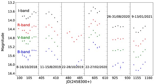
The STV LC of TXS 0506 + 056 in I, R, V, and B bands.
Short-term LCs values.
| ST | Duration | Brightest | Faintest | Mean | Amplitude |
|---|---|---|---|---|---|
| yyyymmdd | Magnitude | Magnitude | Magnitude | Variation(|$\%$|) | |
| ST1 | 20181008-20181016 | 14.26 ± 0.01 | 14.59 ± 0.03 | 14.42 ± 0.03 | 32.87 |
| ST2 | 20190811-20190815 | 14.22 ± 0.01 | 14.67 ± 0.02 | 14.41 ± 0.02 | 44.94 |
| ST3 | 20191022-20191028 | 14.52 ± 0.02 | 14.97 ± 0.02 | 14.73 ± 0.02 | 44.91 |
| ST4 | 20200222-20200227 | 13.98 ± 0.01 | 14.29 ± 0.03 | 14.14 ± 0.03 | 30.87 |
| ST5 | 20210109-20210113 | 14.82 ± 0.02 | 14.88 ± 0.01 | 14.85 ± 0.02 | 5.61 |
| ST6 | 20210827-20210901 | 14.85 ± 0.01 | 15.16 ± 0.03 | 15.02 ± 0.03 | 30.87 |
4.2.2 Long-term flux variability
Fig. 4 illustrates the long-term (LT) LCs of TXS 0506 + 056 in the B, V, R, and I bands over the entire monitoring period. The plot depicts the nightly averaged magnitudes in the respective bands as a function of time. During our monitoring period, the source was detected in the brightest state of R = 13.98 mag on 2020 February 24, while the faintest level detected was R = 15.16 mag on 2021 August 29. The mean magnitudes were 15.62, 15.02, 14.55, and 13.91 in B, V, R, and I bands, respectively. The presence of variability on LT time-scales is clearly evident across all optical wavelengths. Using equation (1), we have estimated very similar variability amplitudes of 117.6 per cent, 137.9 per cent, 117.6 per cent, and 113.8 per cent in B, V, R, and I bands, respectively.

LTV optical (BVRI) light curves of TXS 0506 + 056.
4.3 Spectral variability
The colour–magnitude (CM) relationship serves as a valuable tool for investigating different variability scenarios and gaining a deeper understanding of the origin of blazar emission. In this study, we conducted a search to identify any potential relationship between the source’s colour indices (CIs) with brightness in the R-band and with respect to time. We fitted the plots of the optical (B − V), (B − I), (V − R), and (R − I) CIs with respect to both R-band magnitude and time using straight lines of the form Y = mX + C as shown in Figs 5 and 6, respectively (Pandey et al. 2020a). The values of the parameters related to the colour-time and CM plots are, respectively, provided in the accompanying Tables 5 and 6. In our analysis, we observed modestly significant variations (p < 0.51) in the B − V and B − I colours with respect to the R magnitude. On the other hand, the CIs involving the R-band exhibited very weak trends in the same directions. A positive slope defines a positive correlation between CIs and blazar R magnitude, meaning that the source follows a BWB trend, while a negative slope defines RWB trend (e.g. Gupta et al. 2017, and references therein). We find a negative correlation of the (R − I) CI with time while the B − I colour shows a very weak (about 1.5σ) negative slope. The B − V CI is essentially constant while the V − R one shows a very weak positive trend with time.
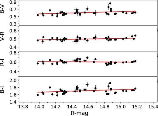
Optical CM plot with respect to R band of TXS 0506 + 056.
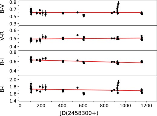
Optical colour variability LCs covering the total observation duration of TXS 0506 + 056.
CM dependencies and CM correlation coefficients on LTV time-scales.
| Colour Index | |$m_1\, ^a$| | |$c_1\, ^a$| | |$r_1\, ^a$| | |$p_1\, ^a$| |
|---|---|---|---|---|
| B − I | 0.083 ± 0.035 | 0.496 | 0.346 | 0.021 |
| R − I | 0.003 ± 0.019 | 0.544 | 0.028 | 0.856 |
| V − R | 0.013 ± 0.007 | 0.313 | 0.238 | 0.118 |
| B − V | 0.066 ± 0.033 | −0.367 | 0.297 | 0.051 |
| Colour Index | |$m_1\, ^a$| | |$c_1\, ^a$| | |$r_1\, ^a$| | |$p_1\, ^a$| |
|---|---|---|---|---|
| B − I | 0.083 ± 0.035 | 0.496 | 0.346 | 0.021 |
| R − I | 0.003 ± 0.019 | 0.544 | 0.028 | 0.856 |
| V − R | 0.013 ± 0.007 | 0.313 | 0.238 | 0.118 |
| B − V | 0.066 ± 0.033 | −0.367 | 0.297 | 0.051 |
am1 = slope and c1 = intercept of CI against R-mag; r1 = Correlation coefficient; p1 = null hypothesis probability.
CV with respect to time on LTV time-scales.
| Colour Index | |$m_1\, ^a$| | |$c_1\, ^a$| | |$r_1\, ^a$| | |$p_1\, ^a$| |
|---|---|---|---|---|
| B − I | −4.251e−05 ± 3.238e−05 | 1.724 | −0.199 | 0.196 |
| R − I | −6.613e−05 ± 1.418e−05 | 0.641 | −0.584 | 3.174e−05 |
| V − R | 1.187e−05 ± 7.137e−06 | 0.491 | 0.249 | 0.104 |
| B − V | 1.172e−05 ± 3.086e−05 | 0.593 | 0.058 | 0.706 |
am1 = slope and c1 = intercept of CI against time; r1 = Correlation coefficient; p1 = null hypothesis probability.
4.4 Spectral energy distribution
Throughout our observation period, we extracted the optical (BVRI) SEDs of the blazar on 44 nights. These SEDs were derived from quasi-simultaneous observations conducted across all four wavebands. For this, we first dereddened the calibrated B, V, R, and I magnitudes by subtracting the Galactic extinction, with Aλ having the following values: AB = 0.392 mag, AV = 0.297 mag, AR = 0.235 mag, and AI = 0.163 mag. The values of Aλ were taken from the NASA Extragalactic Database (NED).4 After applying the necessary dereddening and calibration procedures, the magnitudes in each band were converted into corresponding flux densities Fν that had been corrected for extinction. The optical SEDs of TXS 0506 + 056, in log(ν) versus log(Fν) representation, are plotted in Fig. 7. We measured the source’s faintest and brightest fluxes on 2021 August 29 and 2020 February 24, respectively.
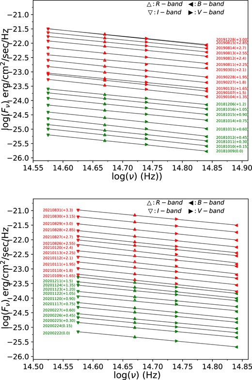
The SED of TXS 0506 + 056 in I, R, V, and B bands.
To determine the optical spectral indices, we fitted each SED with a first-order polynomial model of the form log(Fν) = −α log(ν) + C. The obtained fitting results are presented in Table 7. The values of the spectral indices (α) range from 0.791 ± 0.154 to 1.029 ± 0.194 and their mean was 0.897 ± 0.171. This mean value of the spectral index closely matches previously reported results for TXS 0506 + 056 (Paiano et al. 2018; Hwang et al. 2021).
Straight-line fits to optical SEDs of TeV Blazar TXS 0506 + 056.
| Observation date | |$m_1\, ^a$| | |$c_1\, ^a$| | |$r_1\, ^a$| | |$p_1\, ^a$| | Observation date | |$m_1\, ^a$| | |$c_1\, ^a$| | |$r_1\, ^a$| | |$p_1\, ^a$| |
|---|---|---|---|---|---|---|---|---|---|
| yyyy-mm-dd | yyyy-mm-dd | ||||||||
| 2018-10-09 | 0.925 ± 0.091 | 2.539 | −0.998 | 0.002 | 2020-02-24 | 0.827 ± 0.082 | 1.179 | −0.998 | 0.002 |
| 2018-10-10 | 0.961 ± 0.132 | 3.145 | −0.996 | 0.004 | 2020-02-25 | 0.852 ± 0.091 | 1.616 | −0.998 | 0.002 |
| 2018-10-11 | 0.922 ± 0.083 | 2.651 | −0.998 | 0.002 | 2020-02-26 | 0.825 ± 0.086 | 1.289 | −0.998 | 0.002 |
| 2018-10-12 | 1.005 ± 0.121 | 3.949 | −0.997 | 0.003 | 2020-02-27 | 0.844 ± 0.098 | 1.659 | −0.997 | 0.003 |
| 2018-10-13 | 0.933 ± 0.119 | 3.009 | −0.997 | 0.003 | 2020-11-17 | 0.887 ± 0.103 | 2.365 | −0.997 | 0.003 |
| 2018-10-14 | 0.859 ± 0.081 | 2.031 | −0.998 | 0.002 | 2020-11-20 | 0.824 ± 0.261 | 1.539 | −0.981 | 0.018 |
| 2018-10-15 | 0.921 ± 0.076 | 3.027 | −0.999 | 0.001 | 2020-11-22 | 0.849 ± 0.119 | 1.969 | −0.997 | 0.003 |
| 2018-10-16 | 0.898 ± 0.098 | 2.795 | −0.998 | 0.002 | 2020-11-23 | 0.859 ± 0.205 | 2.213 | −0.991 | 0.009 |
| 2018-12-06 | 0.886 ± 0.069 | 2.672 | −0.999 | 0.001 | 2020-11-24 | 0.917 ± 0.132 | 3.174 | −0.996 | 0.004 |
| 2019-01-04 | 0.957 ± 0.119 | 3.853 | −0.997 | 0.003 | 2020-12-11 | 0.907 ± 0.119 | 2.964 | −0.996 | 0.004 |
| 2019-01-07 | 0.868 ± 0.076 | 2.646 | −0.999 | 0.001 | 2021-01-09 | 0.935 ± 0.205 | 3.468 | −0.997 | 0.012 |
| 2019-01-31 | 0.949 ± 0.055 | 3.814 | −0.999 | 0.001 | 2021-01-10 | 0.917 ± 0.132 | 3.305 | −0.996 | 0.004 |
| 2019-02-27 | 0.911 ± 0.028 | 3.368 | −0.999 | 0.001 | 2021-01-11 | 0.897 ± 0.133 | 3.106 | −0.995 | 0.017 |
| 2019-02-28 | 0.955 ± 0.048 | 4.116 | −0.999 | 0.001 | 2021-01-12 | 0.978 ± 0.152 | 4.371 | −0.998 | 0.002 |
| 2019-03-01 | 0.791 ± 0.154 | 1.807 | −0.993 | 0.007 | 2021-01-13 | 0.845 ± 0.132 | 2.507 | −0.995 | 0.002 |
| 2019-08-11 | 0.898 ± 0.095 | 3.486 | −0.998 | 0.002 | 2021-01-20 | 1.029 ± 0.194 | 5.298 | −0.991 | 0.002 |
| 2019-08-12 | 0.871 ± 0.093 | 3.182 | −0.998 | 0.002 | 2021-08-26 | 0.875 ± 0.097 | 3.107 | −0.998 | 0.002 |
| 2019-08-13 | 0.879 ± 0.094 | 3.363 | −0.998 | 0.002 | 2021-08-27 | 0.917 ± 0.099 | 3.771 | −0.998 | 0.002 |
| 2019-08-14 | 0.891 ± 0.079 | 3.599 | −0.999 | 0.001 | 2021-08-28 | 0.912 ± 0.095 | 3.791 | −0.998 | 0.002 |
| 2019-08-15 | 0.899 ± 0.095 | 2.739 | −0.998 | 0.002 | 2021-08-29 | 0.899 ± 0.102 | 3.699 | −0.998 | 0.002 |
| 2019-12-28 | 0.947 ± 0.095 | 4.469 | −0.998 | 0.002 | 2021-08-30 | 0.859 ± 0.096 | 3.231 | −0.998 | 0.002 |
| 2020-02-22 | 0.847 ± 0.069 | 3.242 | −0.998 | 0.001 | 2021-08-31 | 0.847 ± 0.095 | 3.148 | −0.998 | 0.002 |
am1 = slope and c1 = intercept of log(Fν) and log(ν); r1 = correlation coefficient; p1 = null hypothesis probability.
In Fig. 8, the top and bottom panels display the spectral indices of TXS 0506 + 056 with respect to time and R-band magnitude, respectively. We fitted each panel in Fig. 8 with a first-order polynomial to investigate any variations in the spectral index. The corresponding fitting parameter values are provided in Table 8 The optical spectral index demonstrates a hint of a decreasing trend with time and apparently exhibits a weak positive correlation with the R-band magnitude. However, given the slope of the variation (0.053) and the relatively large error on it (0.022) we cannot have confidence in the reality of this trend.
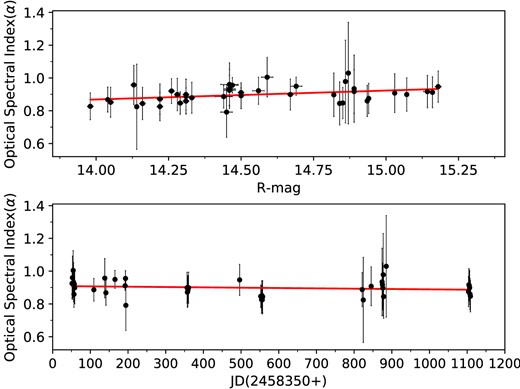
Variation of optical spectral index (α) of TXS 0506 + 056 with respect to R-magnitude (top) and JD (bottom).
Variation of optical spectral index (α), with respect to R-magnitude and LTV time-scale.
| Parameters | m | c | r | p |
|---|---|---|---|---|
| α versus time | −2.26e−05 ± 1.08e−05 | 0.909 | −0.172 | 0.264 |
| α versus Rmag | 0.053 ± 0.022 | 0.123 | 0.362 | 0.016 |
| Parameters | m | c | r | p |
|---|---|---|---|---|
| α versus time | −2.26e−05 ± 1.08e−05 | 0.909 | −0.172 | 0.264 |
| α versus Rmag | 0.053 ± 0.022 | 0.123 | 0.362 | 0.016 |
Notes. m = slope and c = intercept of α against R-mag and JD; r = correlation coefficient; p = null hypothesis probability.
5 DISCUSSION AND CONCLUSIONS
The thermal radiation in blazars emitted by the accretion disc is typically overwhelmed by the Doppler-boosted non-thermal radiation originating from the relativistic jet. As a result, any observed variability is more likely to be explained by models based on the relativistic jet (e.g. Agarwal & Gupta 2015, and references therein). During periods when a blazar exhibits a very low flux state, the observed variability could potentially be attributed to hotspots or instabilities occurring on the accretion disc (e.g. Chakrabarti & Wiita 1993; Mangalam & Wiita 1993). IDV/STV observed in the optical bands can be attributed to the presence of turbulence near a shock in the jet, as well as other irregularities within the jet flow resulting from variations in the outflow parameters (e.g. Marscher 2014; Calafut & Wiita 2015, and references therein).
The micro-level flux variations observed in blazars LCs on IDV time-scales may be attributed to the turbulent plasma flowing at relativistic speeds within the jet (e.g. Marscher 2014; Pollack, Pauls & Wiita 2016) or to mini-jets within the jets (Giannios, Uzdensky & Begelman 2009). Different optical IDV behaviours have been observed in two subclasses of blazars, namely LBLs and HBLs. HBLs display relatively less variability in optical bands on IDV time-scales compared to their amplitude of variability in X-rays and γ-rays (e.g. Heidt & Wagner 1996; Gopal-Krishna et al. 2011; Gaur et al. 2012b; Gupta et al. 2016b, and references therein). The presence of strong magnetic fields within the relativistic jet may be responsible for the different microvariability behaviours observed in the optical bands of both LBLs and HBLs (Romero, Cellone & Combi 1999). The idea is that stronger magnetic fields in HBLs can potentially interrupt the formation of small fluctuations caused by Kelvin–Helmholtz instabilities within relativistic jets. These fluctuations typically interact with shocks in the jets, leading to IDV. However, the generation of very rapid variability can be disrupted if the strength of the magnetic field exceeds the critical value Bc (Romero 2005),
where ne is the local electron density, me is the rest mass of the electron, and γ is the bulk Lorent z factor of the flow. The bulk Lorentz factor γ, and the Doppler factor δ are given by δ = [γ(1 − βcos θ]−1, where βc and θ are the velocity of emitting plasma and jet viewing angle, respectively. For TXS 0506 + 056, |$\theta , \delta , \rm {and} \ \gamma$| are found to be 8°–20°, 2–9, and ∼ 5, respectively (Kun, Biermann & Gergely 2019; Li et al. 2020; Sumida et al. 2022). The local electron density ne can be estimated using broad-band multiwavelength SED of blazars. However, for TXS 0506 + 056 a broad-band multiwavelength SED is not available, so we took the average value of ne for other possible potential neutrino loud TeV blazars (e.g. Mrk 421, Mrk 501, 1ES 1426 + 428, PKS 2155-304, 1ES 2344 + 514, etc.; Neronov & Semikoz 2002). The electron density ne of these blazars are found to be in the range of 0.3–1.45 electrons cm−3 (Abdo et al. 2011a, b; Cerruti et al. 2012; Prandini et al. 2019; MAGIC Collaboration et al. 2020). Considering these parameter values, we get B ≈ 0.1 G. As TXS 0506 + 056 is a TeV blazar, it is expected to have B > Bc that, within this scenario, would inhibit the development of the small-scale structures that could yield IDV in the optical LCs.
Changes in colour or spectral index can aid in understanding of the emission mechanisms in blazars. As mentioned earlier, three distinct types of behaviour can be observed in the CMD: redder-when-brighter (RWB), bluer-when-brighter (BWB), and achromatic. The BWB trend is commonly observed in BL Lacs, whereas the RWB trend is typically followed by FSRQs (e.g. Gaur, Gupta & Wiita 2012a; Gaur et al. 2015b). Synchrotron models dominated by one component can explain the BWB behaviour if the energy distribution of injected fresh electrons, which cause an increase in flux, is harder (Kirk, Rieger & Mastichiadis 1998). Another possible explanation for BWB behaviour involves precession of the jet, causing variations in the Doppler factor that affect the ‘convex’ spectrum (Villata et al. 2004b). During our observations, we consistently observed that TXS 0506 + 056 followed the BWB trend. This suggests that the increasing flux can be attributed to jet synchrotron emission, very possibly indicating an enhancement in particle acceleration efficiency (Agarwal et al. 2015). This BWB trend is seen in Fig. 8 that illustrates spectral steepening as the magnitude increases. This trend can also be explained by a two component emission picture: one is a stable component (αconstant), while the other is a variable component with a flatter slope (α1). When the variable component dominates over the stable component then chromatic behaviours are exhibited. On shorter timescales, optical variations are predominantly influenced by strong chromatic components, while longer term optical variations can be attributed to a mildly chromatic component (Villata et al. 2004a).
The spectral and flux variations observed in TXS 0506 + 056 may offer valuable insights into the evolutionary processes occurring in radio loud AGN (e.g. Barth, Ho & Sargent 2002; Fan 2003). In an accretion disc-based model, the shortest variability time-scale is connected to the time it takes for light to traverse the variable region which is directly related to the BH mass (Bachev, Strigachev & Semkov 2005). The likelihood of detecting variability in blazars becomes greater as the duration of observations increases. For instance, extending the observation period from ≤ 3 to ≥ 6 h resulted in an increase in the probability of identifying IDV in blazars from 64 per cent to 82 per cent (Gupta & Joshi 2005).
In this study, we conducted an analysis of optical photometric data obtained from seven ground-based telescopes, covering the period from October 2018 to August 2021, for the TeV blazar TXS 0506 + 056. This study represents the first comprehensive investigation of the temporal and spectral behaviour of this source across a wide range of time-scales within the optical domain. We examined a total of 35 R-band, 14 V-band, 7 I-band, and 6 B-band IDV LCs using two powerful and robust statistical methods, namely the nested ANOVA test and the power-enhanced F-test. During the period of our observations, we observed significant variability in the R-band on 8 nights and in the V-band on 2 nights. However, no IDV was detected in the B and I bands for which we took many fewer measurements. Additionally, we observed a variation in the (V − R) colour within only one night throughout the entire observation period. The DCs we measured for the R and V bands are 22.8 per cent and 14.3 per cent, respectively. So, from our IDV analysis, we conclude that optical LCs of TXS 0506 + 056 are either constant or show nominal variations on IDV time-scales. The blazar TXS 0506 + 056 did not show large-amplitude variations during our monitoring period. One important caveat is that the duration of our observations ranges from 1 to 6 h, so it is certainly possible that if more of our nightly observations had covered longer periods we would have seen more frequent IDV. In a statistical study of the optical IDV of blazars, it was found that chances of detection of IDV is 60–65 per cent if observations are performed for less than 6 h, but if the blazar is observed for more than 6 h, the chance of detecting IDV is 80–85 per cent (Gupta & Joshi 2005).
By analysing the ACFs, we were able to identify evidence of variability time-scales on 2020 November 20, in both the V and R bands. The variability time-scales were determined to be 3.50 h in the V band and 3.06 h in the R band reported in Table 3 and shown in Fig. 2. To obtain an upper limit for the size (R) of the emission region, we apply the simple causality constraint,
where δ is the Doppler factor. The values of δ for TXS 0506 + 056 have been estimated to be between 2 and 9 using radio very long baseline interferometry/very long baseline array data in the frequency range 8 GHz to 43 GHz (Kun, Biermann & Gergely 2019; Li et al. 2020; Sumida et al. 2022). Using that range of Doppler factor values, taking z = 0.3365 (Paiano et al. 2018), and employing the shortest variability timescale we found (tvar = 11.02 ks in the R band), and employing equation (3), we obtain that the size of the emission region is in the range of 4.95 |$\times \rm {10}^{14}$|cm – 2.23 × 1015 cm.
To determine the optical spectral index (α), we constructed optical SEDs using quasi-simultaneous observations in the B, V, R, and I bands at different epochs. The analysis revealed a weak positive correlations between the optical spectral index (α) and R-band magnitude. Over the LTV time-scale, the weighted mean value of α was determined to be 0.897 ± 0.171. Since TXS 0506 + 056 is the best case for a blazar producing neutrino fluxes it should remain a priority target for continuing observations in all bands.
ACKNOWLEDGEMENTS
We thank the anonymous reviewer for very useful comments that helped us to improve the manuscript. ACG is partially supported by Chinese Academy of Sciences (CAS) President’s International Fellowship Initiative (PIFI) (grant no. 2016VMB073). This research was partially supported by the Bulgarian National Science Fund of the Ministry of Education and Science under grants KP-06-H28/3 (2018), KP-06-H38/4 (2019), KP-06-KITAJ/2 (2020) and KP-06-H68/4 (2022). The Skinakas Observatory is a collaborative project of the University of Crete, the Foundation for Research and Technology – Hellas, and the Max-Planck-Institut für Extraterrestrische Physik. HG acknowledges financial support from the Department of Science and Technology (DST), Government of India, through INSPIRE faculty award IFA17-PH197 at ARIES, Nainital, India. Based on data acquired at Complejo Astronómico El Leoncito, operated under agreement between the Consejo Nacional de Investigaciones Cientificas y Técnicas de la República Argentina and the National Universities of La Plata, Córdoba, and San Juan.
DATA AVAILABILITY
The data of this article will be shared after one year of the publication of the paper at a reasonable request to the first author.
Footnotes
Image Reduction and Analysis Facility (IRAF) is distributed by the National Optical Astronomy Observatory, which is operated by the Association of Universities for Research in Astronomy (AURA) under a cooperative agreement with the National Science Foundation.
Dominion Astrophysical Observatory Photometry
