


ABSTRACT
We report the discovery of two mini-Neptunes in near 2:1 resonance orbits (P = 7.610303 d for HIP 113103 b and P = 14.245651 d for HIP 113103 c) around the adolescent K-star HIP 113103 (TIC 121490076). The planet system was first identified from the TESS mission, and was confirmed via additional photometric and spectroscopic observations, including a ∼17.5 h observation for the transits of both planets using ESA CHEOPS. We place ≤4.5 min and ≤2.5 min limits on the absence of transit timing variations over the 3 yr photometric baseline, allowing further constraints on the orbital eccentricities of the system beyond that available from the photometric transit duration alone. With a planetary radius of Rp = |$1.829_{-0.067}^{+0.096}$| R⊕, HIP 113103 b resides within the radius gap, and this might provide invaluable information on the formation disparities between super-Earths and mini-Neptunes. Given the larger radius Rp = |$2.40_{-0.08}^{+0.10}$| R⊕ for HIP 113103 c, and close proximity of both planets to HIP 113103, it is likely that HIP 113103 b might have lost (or is still losing) its primordial atmosphere. We therefore present simulated atmospheric transmission spectra of both planets using JWST, HST, and Twinkle. It demonstrates a potential metallicity difference (due to differences in their evolution) would be a challenge to detect if the atmospheres are in chemical equilibrium. As one of the brightest multi sub-Neptune planet systems suitable for atmosphere follow up, HIP 113103 b and HIP 113103 c could provide insight on planetary evolution for the sub-Neptune K-star population.
1 INTRODUCTION
Super-Earths (1 R⊕ < Rp ≤ 1.5 R⊕) and mini-Neptunes (1.5 R⊕ < Rp ≤ 4 R⊕) are the most common planets found around sun-like stars (referred to as sub-Neptunes hereafter), especially those residing in close-in orbits (Howard et al. 2012; Fressin et al. 2013; Bergsten et al. 2022), despite having no analogues in our own Solar System. These planets bridge the gap between rocky Earth-like worlds and gaseous Neptunes (e.g. Fulton et al. 2017). The Transiting Exoplanet Survey Satellite (TESS; Ricker et al. 2015) mission continues to expand our repertoire for sub-Neptunes, in particular those orbiting bright nearby stars. These discoveries have led to precise radius and mass constraints for a significant number of sub-Neptunes (e.g. Dragomir et al. 2019; Gandolfi et al. 2019; Cloutier et al. 2020; MacDougall et al. 2021; Sozzetti et al. 2021; Gan et al. 2022; Lubin et al. 2022), as well as the possibility of in-depth atmospheric characterizations that reveal the origins and evolutionary pathways of this population (e.g. Osborn et al. 2021; Kawauchi et al. 2022).
Hypothesized planet formation pathways for sub-Neptunes [see Bean, Raymond & Owen (2021) for more information] will exhibit observable differences that are accessible with the new generation of space and ground based facilities (e.g. Greene et al. 2016; Tinetti et al. 2018). Depending on what occurs after dissipation of the gas disc, sub-Neptunes may not contain enough mass to gravitationally maintain their primordial atmosphere (e.g. Walker 1986; Lopez, Fortney & Miller 2012; Ginzburg, Schlichting & Sari 2018; Kite & Barnett 2020; Kite et al. 2020). The rate of mass-loss post-formation is strongly dependent on the irradiation the planets receive from their host stars. Planets receiving strong XUV irradiation may be more likely to lose their primordial envelope (e.g. Owen & Jackson 2012; Howe & Burrows 2015; Mordasini 2020; Ketzer & Poppenhaeger 2022).
The next generation space-based telescopes [commencing with the James Webb Space Telescope (JWST); Greene et al. (2016)] will be capable of characterizing the atmospheres of sub-Neptunes, and many are prioritizing wavelength regions towards the infrared (e.g. Tinetti et al. 2018; Stotesbury et al. 2022). Obstruction by haze and clouds are minimized at longer wavelengths, and early JWST observations have already demonstrated its invaluable retrieval capabilities for exoplanets atmospheres (e.g. Ahrer et al. 2023; Alderson et al. 2023; Feinstein et al. 2023; Rustamkulov et al. 2023; Tsai et al. 2023). Prior to the launch of these next generation telescopes, some attempts of measuring sub-Neptune atmospheres have resulted in observations obscured by haze (e.g. Kreidberg et al. 2014; Mugnai et al. 2021); however, there have been notable exceptions which suggest predominant H/He envelopes (e.g. Benneke et al. 2019; Tsiaras et al. 2019; Edwards et al. 2022; Orell-Miquel et al. 2022). Due to their size, observing sub-Neptune atmospheres is challenging in comparison to their larger Jovian counterparts, particularly around FGK stars. Therefore, the most suitable population of sub-Neptunes for atmosphere analysis are those residing in close orbits to bright host stars. In the known FGK planet population, there are only a handful of sub-Neptunes that meet these requirements (e.g. Winn et al. 2011; Gandolfi et al. 2018; Dragomir et al. 2019; Teske et al. 2020), with samples dwindling further when only considering multisub-Neptune planet systems (e.g. Rodriguez et al. 2018; Delrez et al. 2021; Scarsdale et al. 2021; Barragán et al. 2022). It is therefore vital to identify sub-Neptunes with short periods around bright stars, as these candidates will lead the research towards understanding the formation pathways of this vast sub-class.
In this paper, we report the discovery of two sub-Neptunes that orbit at a 2:1 resonance around the bright K-star HIP 113103 (TIC 121490076). The initial observations with TESS and subsequent follow up with the CHaracterising ExOPlanets Satellite (CHEOPS; Benz et al. 2021) and ground-based facilities are outlined in Section 2, while our global model fit to constrain the physical parameters of each planet are outlined in Section 3. The physical properties of HIP 113103 are discussed in Section 4, while the elimination of false positive scenarios are outlined in Section 5. Our Results and Discussion are presented in Section 6 followed by our Conclusion in Section 7, respectively.
2 OBSERVATIONS
2.1 Candidate identification with TESS
The transiting planets around HIP 113103 were first identified by observations from TESS. Observations for HIP 113103 were obtained via the 30 min cadence Full Frame Images (FFI) from Sector 1 Camera 2, and via 10 min FFIs and 2 min target pixel stamps from Sector 28 Camera 2.
The transit signals around HIP 113103 were identified as part of a search for planets around young active field stars (Zhou et al. 2021) via public FFI light curves from the MIT Quick look pipeline (Huang et al. 2020a, b). The target star was identified as a potential young star via its high amplitude rotational modulation using the 10 min FFI light curves from Sector 28. The combined FFI light curves of Sector 1 and 28 were first modeled and detrended via a spline interpolation (Vanderburg & Johnson 2014), and searched for transit signals via the box-least-squared (BLS) procedure (Kovács, Zucker & Mazeh 2002). Two candidate signals are detected by BLS, one at ≈ 7.61 d with a signal to noise of 14, the other at ≈ 14.24 d with a signal to noise of 12.79. Both signals crossed the recommended threshold to be classified as a threshold crossing event (TCE) as defined by the TESS Objects of Interest (TOI) team (Guerrero et al. 2021). We vetted the data for both TCEs to rule out astrophysical false positives due to blending from nearby eclipsing binaries outside of the centre pixel. We found that transit depth derived from different apertures are similar, and found no obvious blending sources when examining light curves from individual pixels in and around the aperture. We then promoted both TCEs for further follow up via CHEOPS (Section 2.2) and ground based instruments (Sections 2.3 and 2.4).
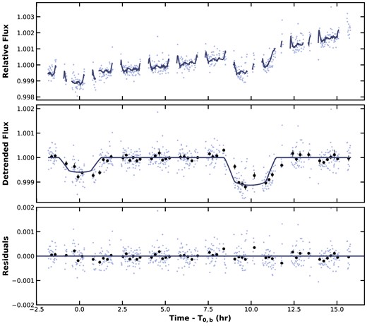
To refine the orbital and physical characteristics of the planets in our global model (Section 3), we use of the debelended Sector 28 target pixel stamp (TPF) 2-min cadence Simple Aperture Photometry (SAP) light curves (Twicken et al. 2010; Morris et al. 2020), performing the deblending using the contamination keywords in the TPF files. These light curves originate from the Science Processing Operations Center (SPOC; Jenkins et al. 2016) at NASA Ames Research Center, and are made available via the the Mikulski Archive for Space Telescopes (MAST).1 HIP 113103 exhibits significant rotational modulation due to spot activity on the stellar surface. To ensure proper propagation of the uncertainties associated with these noise sources, we model the rotational modulation and spacecraft systematics alongside the transiting planet signals. We use the deblended simple aperture SPOC light curves in this simultaneously detrending procedure. Following Vanderburg et al. (2019), we describe these signals as a linear combination of the spacecraft quarternions, the top seven covariant basis vectors, and a set of 20 cosine and sine functions at frequencies up to the TESS orbital period of 13 d (also see Mazeh & Faigler 2010; Huang, Bakos & Hartman 2013). Fig. 1 shows the TESS discovery light curve before and after the removal of the stellar and instrumental effects, while Fig. 2 and Fig. 3, 3, 4 show the individual transit light curves centred at HIP 113103 b and HIP 113103 c respectively. Fig. 4 shows the phase folded TESS transit light curves for each planet.
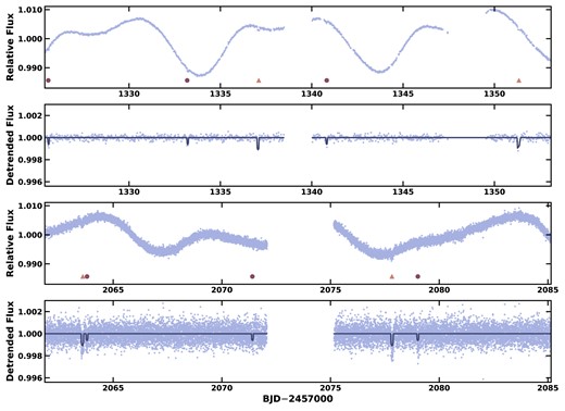
The TESS light curves before and after the removal of spot modulated rotational signals. The light curves of HIP 113103 from Sector 1 via FFI observations were observed at 30 min cadence (Panels 1 and 2), and from Sector 28 TPF observations at 2 min (Panels 3 and 4). Transits by HIP 113103 b and HIP 113103 c are illustrated via a circle and triangle respectively. The best-fitting transit model is displayed in navy.
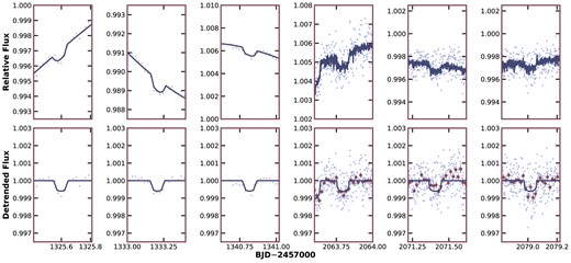
The TESS light curves centred on the transits of HIP 113103 b. The top panel shows the pre-detrending, the bottom panel shows the post-detrending light curves, after the removal of spot modulated rotational signal from HIP 113103. Columns 1–3 were observed at 30-min cadence during Sector 1, while 4–6 were observed at 2-min cadence from Sector 28. The best-fitting transit model is displayed in navy, and the detrended transits at 2-min cadence have been binned in 10-min intervals to illustrate the precision of TESS.
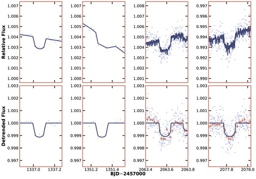
The TESS light curves centred on the transits of HIP 113103 c. The top panel shows the pre-detrending, the bottom shows the post-detrending light curve, after the removal of spot modulated rotational signal from HIP 113103. Columns 1–2 were observed at 30-min cadence during Sector 1, while 3–4 were observed at 2-min cadence during Sector 28. The best-fitting transit model is displayed in navy, and the detrended transits at 2-min cadence have been binned in 10-min intervals to illustrate the precision of TESS.
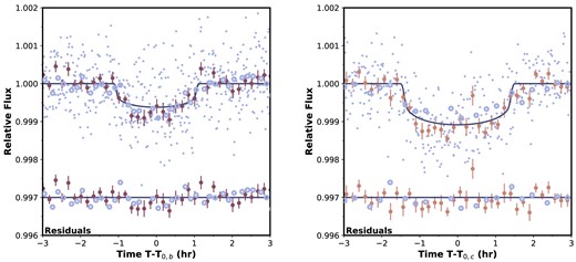
Phase folded TESS transit light curves for HIP 113103 b (left) and HIP 113103 c (right). The light blue open circles represent 30-min cadenced observations, while the light blue filled points represent the 2-min cadenced observations. The points with error bars show the binned 2-min light curves at 10-min cadence. The best-fitting models are over plotted. The binned residuals are plotted at the bottom, vertically offset by 0.003 in flux for clarity.
2.2 CHEOPS follow-up photometry
Although we detected HIP 113103 b and HIP 113103 c through TESS, additional observations with higher precision are required to confirm and constrain the radius and ephemerides values for both planets. We therefore use the CHEOPS mission to observe the primary transit of both planets during a single observing window. CHEOPS is a visible to infrared (|$0.4 \ \mu\text{m}-1.1 \ \mu\text{m}$|) 0.32-m Ritchey–Chretien telescope located in a 700-km geocentric Sun-synchronous orbit. It is capable of capturing high-precision photometry of exoplanets around bright stars, with the corresponding CHEOPS mission focusing on the radius refinement of super-Earths and sub-Neptunes (Benz et al. 2021).
The CHEOPS observation (observation ID: 1901592) was obtained between 2022 September 9 20:31 and 2022 September 10 14:06 UTC (10 orbits over ∼17.5 h), with a ∼5 h baseline between ingress and egress of both transits. At an exposure time of 60 s, 700 frames are obtained, with 10 frames affected by stray light and Earth occultation. This observation of a near-simultaneous transit for HIP 113103 b and HIP 113103 c was possible only because of the near 2:1 resonance of the system.
The low Earth orbit nadir-locked orientation of CHEOPS naturally induces field rotation over the course of a spacecraft-orbit, and results in correlated systematics in the observed light curve. We modelled these effects alongside the transit model as part of our global modelling (Section 3). The spacecraft signals are modelled as a linear combination of the sky background, smear, contamination, pixel X and Y drifts, and a set of four sine and cosine functions at frequencies up to four times the spacecraft orbital period as a function of the spacecraft roll angle.
Fig.5 shows the raw and detrended CHEOPS light curves, and the model describing the instrumental signals that were removed from the raw light curve.
The follow-up CHEOPS observations of HIP 113103 b (first transit) and HIP 113103 c (second transit) taken over a single ∼17.5 h visit. The top panel displays the raw light curves from the optimal aperture extraction. The model describing the planetary transits and the instrumental effects is overplotted via the navy line (see Section 3). The middle panel shows the detrended CHEOPS light curve after removal of the instrumental spacecraft orbit induced variations and the best-fitting transit model. The transits are binned in 10-min intervals to illustrate the precision of CHEOPS. The bottom panel illustrates the residuals of the data.
2.3 Ground-based follow-up photometry
In addition to space-based observations, we also obtained ground-based seeing limited photometry through the TESS Follow-up Observing Program (TFOP) photometry science working group (SG1) to detect the transits of both planets and further rule out other nearby targets contaminating the detection.
Two transits of both HIP 113103 b and HIP 113103 c were obtained using the Las Cumbres Observatory Global Telescope (LCOGT Brown et al. 2013) facility. We used the 1-m telescopes of the LCOGT network for these observations. Each telescope is equipped with a sinistro|$4\, \mathrm{K}\times 4\, \mathrm{K}$| andor EM CCD camera, yielding a field of view of 5.7 arcmin and a pixel scale of |$0.34^{\prime \prime }\, \mathrm{pixel}^{-1}$|. These observations are able to detect the transits of both planets with high significance, and determine that the transit depths are consistent with those derived from TESS and CHEOPS. The images were calibrated using the standard LCOGT banzai pipeline (McCully et al. 2018) and the differential photometric data was extracted using astroimagej (Collins et al. 2017). Given Gaia DR3 catalogue shows that no other stars are within 10 arcsec of HIP 113103, we determine that the transit signals most likely originated from the target star. The light curves are detrended simultaneously against the airmass in our global fit. Fig. 6 shows the detrended light curves against their respective model light curve from our global model fit. The observations are detailed as follows:
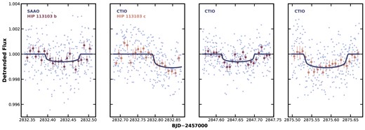
The ground-based detrended photometric follow-up observations of HIP 113103 b and HIP 113103 c, as obtained with the Las Cumbres Observatory 1-m telescopes at the South African Astronomical Observatory and the Cerro Tololo Interamerican Observatory (all in zs filter). The best-fitting transit model is represented via the navy line, while each transit has been binned in 10-min intervals to illustrate the precision of the LCO telescopes.
A full transit of HIP 113103 b was obtained via the 1-m telescope at the South African Astronomical Observatory (SAAO) on UT 2022-09-09 with a 5.5 arcsec radius aperture using the zs filter. On UT 2022-09-10, a partial transit of HIP 113103 c, including ingress, was obtained from the Cerro Tololo Interamerican Observatory (CTIO) node with a 6.2 arcsec radius aperture using the zs filter. An additional full transit for both HIP 113103 b and HIP 113103 c were obtained from the CTIO node on UT 2022-09-10 and UT 2022-10-22. Both transits were obtained with the zs filter, with an aperture size of 8.2 arcsec and 7.0 arcsec for HIP 113103 b and HIP 113103 c, respectively. Table 1 displays all the photometric transit observations analysed in this work.
A summary of all ground-based photometric transit observations for HIP 113103 b and HIP 113103 c.
| Target | Instrument | Date (UT) | Filter | Aperture |
|---|---|---|---|---|
| HIP 113103 b | SAAO 1.0 m | 2022-09-09 | zs | 5.5 arcmin |
| HIP 113103 c | CTIO 1.0 m | 2022-09-10 | zs | 6.2 arcmin |
| HIP 113103 b | CTIO 1.0 m | 2022-09-25 | zs | 8.2 arcmin |
| HIP 113103 c | CTIO 1.0 m | 2022-10-22 | zs | 7.0 arcmin |
These instruments are involved in the LCOGT consortium.
2.4 Spectroscopic characterization
To characterize the stellar properties of the host star and validate the planetary-nature of the transiting candidates, we obtained a series of reconnaissance spectroscopic observations of HIP 113103 with a set of southern spectroscopic facilities.
The stellar atmospheric parameters were derived by matching each observation against a library of ∼10 000 observed spectra previously classified through the Spectroscopic Classification Pipeline (Buchhave et al. 2012). The library is interpolated via a gradient boosting regressor model, from which the best-fitting spectral parameters were determined (Zhou et al. 2021). We found a best-fitting effective temperature of Teff = 4930 ± 100 K, surface gravity of log g = 4.6 ± 0.1 dex, metallicity of [m/H] = −0.1 ± 0.1 dex, and projected rotational broadening of |$v\sin I_\star = 3\pm 1\, \mathrm{km\, s}^{-1}$| for HIP 113103. We note that the rotational velocity is less than the instrument broadening, and the reported value is likely an upper limit of the true rotation velocity.
In addition, we obtained eight observations of HIP 113103 using the CHIRON facility on the SMARTS 1.5-m telescope located at Cerro Tololo Inter-American Observatory, Chile (Tokovinin et al. 2013). CHIRON is a fibre-fed echelle spectrograph with a resolving power of R ∼ 80 000 over the wavelength range of 4100–8700 Å. We use the extracted spectra from CHIRON reduced via the standard pipeline as per Paredes et al. (2021). The radial velocities are derived from each observation via a least-squares deconvolution of the spectra against a synthetic template generated at the atmospheric parameters of the target star (Donati et al. 1997). The generated line profiles are modelled via a combination of kernels describing the rotational, macroturbulent, and instrument broadening effects (following Gray & Corbally 1994).
We also obtained 10 epochs of spectroscopic observations from the Minerva-Australis array. Minerva-Australis is an array of four identical 0.7-m telescopes, located at Mt Kent Observatory, Australia. The light from all four telescopes are combined into a single kiwispec high resolution echelle spectrograph, with a resolving power of R ∼ 80 000 over the wavelength region of 4800–6200 Å (Barnes et al. 2012; Addison et al. 2019). Wavelength corrections are provided by two simultaneous fibers adjacent to the object fibers, which pass light from a quartz lamp through an iodine cell. Relative radial velocities are derived by a cross correlation between each individual observation and an averaged spectrum of the set of spectra available for the target. These relative velocities are then shifted to the mean absolute velocity of the averaged spectrum. These velocities are also presented in Table 2.
Radial velocity measurements of HIP 113103.
| BJD | RV (km s− 1) | σRV (km s− 1) | Instrument |
|---|---|---|---|
| 2459171.60440 | 12.813 | 0.035 | CHIRON |
| 2459174.59126 | 12.864 | 0.024 | CHIRON |
| 2459176.58998 | 12.824 | 0.022 | CHIRON |
| 2459178.62741 | 12.858 | 0.026 | CHIRON |
| 2459180.55586 | 12.818 | 0.029 | CHIRON |
| 2459182.53304 | 12.830 | 0.034 | CHIRON |
| 2459184.55875 | 12.854 | 0.026 | CHIRON |
| 2459186.62126 | 12.877 | 0.022 | CHIRON |
| 2459917.93684 | 13.370 | 0.022 | Minerva-Australis |
| 2459917.95510 | 13.425 | 0.019 | Minerva-Australis |
| 2459924.93091 | 13.377 | 0.015 | Minerva-Australis |
| 2459924.94916 | 13.382 | 0.020 | Minerva-Australis |
| 2459930.93397 | 13.356 | 0.038 | Minerva-Australis |
| 2459930.95226 | 13.406 | 0.020 | Minerva-Australis |
| 2459942.92801 | 13.384 | 0.019 | Minerva-Australis |
| 2459942.94630 | 13.407 | 0.018 | Minerva-Australis |
| 2460046.29239 | 13.435 | 0.035 | Minerva-Australis |
| 2460046.31065 | 13.409 | 0.014 | Minerva-Australis |
The Minerva-Australis observations have per-point uncertainties of 10–20 m s−1, and are comparable to those obtained from CHIRON. We do not detect significant radial velocity variations at the 20 m s−1 level, consistent with the expected low mass of the planets around HIP 113103. The observations therefore remain consistent with a lack of detection of the radial velocity orbit, as is expected given the velocity uncertainties and the expected orbit amplitude. The line profiles exhibit no visible variations indicative of blend scenarios. In scenarios where the transit is induced by a background eclipsing binary, we would often observe correlations between the rotational broadening velocity and the radial velocities, with the apparent broadening at its maximum at the extremities of the velocity curve. We observe no such correlation for HIP 113103, with the exposure to exposure scatter in the rotational broadening of 0.2 km s−1.
In addition, two archival spectra were obtained from the European Southern Observatory (ESO) HARPS facility on the ESO 3.6-m telescope in La Silla, Chile (Mayor et al. 2003). The observations have a spectral resolution of R = 120 000 over the spectral range of 3780–6910 Å. We make use of the two archival observations, obtained in 2010 and 2013, to further classify the host star atmospheric properties. To calculate the spectroscopic parameters, we make use of the zaspe package (Brahm et al. 2017) and its associated custom spectral library computed from the Castelli & Kurucz (2004) model atmospheres. We find a mean effective temperature of Teff = 4800 ± 60 K, surface gravity of log g = 4.47 ± 0.05 dex, and metallicity of [m/H] = 0.0 ± 0.05 dex, with uncertainties adapted from the uncertainty floor as per Brahm et al. (2017). We do not incorporate the HARPS observations towards our spectroscopic parameters due to the sample being too small. We instead adopt the CHIRON and Minerva-Australis spectra for our spectroscopic parameters, as we were able to test the self consistency of our parameters via its scatter from spectrum to spectrum (as presented in Table 3).
The physical properties of HIP 113103.
| Parameter | Value | Source |
|---|---|---|
| Identifiers|$\ldots \ldots \ldots \ldots \ldots \ldots \ldots \ldots $| | HIP 113 103 | |
| TIC 121 490 076 | ||
| TYC 8011-00766-1 | ||
| 2MASS J22541736-4300372 | ||
| Gaia DR2 6 541 360 574 788 758 016 | ||
| Astrometry | ||
| RA |$\ldots \ldots \ldots \ldots \ldots \ldots \ldots \ldots $| | 22h54m17s.37 | Gaia Collaboration (2022) |
| Dec. |$\ldots \ldots \ldots \ldots \ldots \ldots \ldots \ldots $| | −43°00′37″.25 | Gaia Collaboration (2022) |
| Parallax (mas) |$\ldots \ldots \ldots \ldots \ldots \ldots \ldots \ldots $| | 21.61785 ± 0.00024 | Gaia Collaboration (2022) |
| Proper motion | ||
| Gaia (2016.4) RA proper motion (mas yr−1) |$\ldots \ldots \ldots \ldots \ldots \ldots \ldots \ldots $| | 1.995 ± 0.020 | Gaia Collaboration (2022) |
| Gaia (2016.3) Dec. proper motion (mas yr−1) |$\ldots \ldots \ldots \ldots \ldots \ldots \ldots \ldots $| | 27.384 ± 0.021 | Gaia Collaboration (2022) |
| Hipparcos (1991.2) RA proper motion (mas yr−1) |$\ldots \ldots \ldots \ldots \ldots$| | 2.2 ± 1.5 | Perryman et al. (1997) |
| Hipparcos (1991.4) Dec. proper motion (mas yr−1) |$\ldots \ldots \ldots \ldots \ldots$| | 27.1 ± 1.3 | Perryman et al. (1997) |
| Hipparcos-Gaia average RA proper motion (mas yr−1) |$\ldots \ldots \ldots $| | 2.032 ± 0.048 | Brandt (2021) |
| Hipparcos-Gaia average Dec. proper motion (mas yr−1) |$\ldots \ldots \ldots \ldots $| | 27.396 ± 0.038 | Brandt (2021) |
| Photometry | ||
| TESS (mag) |$\ldots \ldots \ldots \ldots \ldots \ldots \ldots \ldots $| | 8.9988 ± 0.0063 | Stassun et al. (2019) |
| B (mag) |$\ldots \ldots \ldots \ldots \ldots \ldots \ldots \ldots $| | 10.907 ± 0.033 | Høg et al. (2000) |
| V (mag) |$\ldots \ldots \ldots \ldots \ldots \ldots \ldots \ldots $| | 9.95 ± 0.03 | Høg et al. (2000) |
| J (mag) |$\ldots \ldots \ldots \ldots \ldots \ldots \ldots \ldots $| | 8.195 ± 0.03 | Skrutskie et al. (2006) |
| H (mag) |$\ldots \ldots \ldots \ldots \ldots \ldots \ldots \ldots $| | 7.67 ± 0.042 | Skrutskie et al. (2006) |
| K (mag) |$\ldots \ldots \ldots \ldots \ldots \ldots \ldots \ldots $| | 7.557 ± 0.031 | Skrutskie et al. (2006) |
| Gaia G (mag) |$\ldots \ldots \ldots \ldots \ldots \ldots \ldots \ldots $| | 9.6175 ± 0.0018 | Gaia Collaboration (2022) |
| GaiaBP (mag) |$\ldots \ldots \ldots \ldots \ldots \ldots \ldots \ldots $| | 10.1491 ± 0.0033 | Gaia Collaboration (2022) |
| GaiaRP (mag) |$\ldots \ldots \ldots \ldots \ldots \ldots \ldots \ldots $| | 8.9353 ± 0.0039 | Gaia Collaboration (2022) |
| WISE W1 (mag) |$\ldots \ldots \ldots \ldots \ldots \ldots \ldots \ldots $| | 7.398 ± 0.033 | Cutri & et al. (2012) |
| WISE W2 (mag) |$\ldots \ldots \ldots \ldots \ldots \ldots \ldots \ldots $| | 7.538 ± 0.02 | Cutri & et al. (2012) |
| WISE W3 (mag) |$\ldots \ldots \ldots \ldots \ldots \ldots \ldots \ldots $| | 7.489 ± 0.017 | Cutri & et al. (2012) |
| WISE W4 (mag) |$\ldots \ldots \ldots \ldots \ldots \ldots \ldots \ldots $| | 7.395 ± 0.132 | Cutri & et al. (2012) |
| Kinematics and position | ||
| U (km s−1) |$\ldots \ldots \ldots \ldots \ldots \ldots \ldots \ldots $| | 5.00 ± 0.17 | Propagated from Gaia1 |
| V (km s−1) |$\ldots \ldots \ldots \ldots \ldots \ldots \ldots \ldots $| | 4.635 ± 0.031 | Propagated from Gaia1 |
| W (km s−1) |$\ldots \ldots \ldots \ldots \ldots \ldots \ldots \ldots $| | −13.89 ± 0.32 | Propagated from Gaia1 |
| Distance (pc) |$\ldots \ldots \ldots \ldots \ldots \ldots \ldots \ldots $| | 46.212 ± 0.086 | This paper |
| γCHIRON (km s−1) |$\ldots \ldots \ldots \ldots \ldots \ldots \ldots \ldots $| | |$12.845_{-0.013}^{+0.012}$| | This paper |
| γMINERVA (km s−1) |$\ldots \ldots \ldots \ldots \ldots \ldots \ldots \ldots $| | |$13.395_{-0.011}^{+0.010}$| | This paper |
| JitterCHIRON (m s−1) |$\ldots \ldots \ldots \ldots \ldots \ldots \ldots \ldots $| | |$16_{-11}^{+20}$| | This paper |
| JitterMINERVA (m s−1) |$\ldots \ldots \ldots \ldots \ldots \ldots \ldots \ldots $| | |$13_{-9}^{+14}$| | This paper |
| Physical properties | ||
| M⋆ (M⊙) |$\ldots \ldots \ldots \ldots \ldots \ldots \ldots \ldots $| | 0.761 ± 0.038 | This paper |
| R⋆ (R⊙) |$\ldots \ldots \ldots \ldots \ldots \ldots \ldots \ldots $| | 0.742 ± 0.013 | This paper |
| Teff (K) |$\ldots \ldots \ldots \ldots \ldots \ldots \ldots \ldots $| | 4930 ± 100 | This paper |
| log g (cgs) |$\ldots \ldots \ldots \ldots \ldots \ldots \ldots \ldots $| | 4.6 ± 0.1 | This paper |
| [m/H] |$\ldots \ldots \ldots \ldots \ldots \ldots \ldots \ldots $| | −0.1 ± 0.1 | This paper |
| vsin i (km s−1) |$\ldots \ldots \ldots \ldots \ldots \ldots \ldots \ldots $| | 3 ± 1 | This paper |
| Rotation period (d) |$\ldots \ldots \ldots \ldots \ldots \ldots \ldots \ldots $| | 9.92 ± 0.23 | This paper |
| Gyrochronology age (Myr) |$\ldots \ldots \ldots \ldots \ldots \ldots \ldots \ldots $| | |$470_{-110}^{+170}$| | Based on the gyrochronology relationship from Bouma, Palumbo & Hillenbrand (2023) |
| Limb darkening coefficients (TESSu1) |$\ldots \ldots \ldots \ldots \ldots \ldots \ldots \ldots $| | 0.463 ± 0.021 | Claret (2017) |
| Limb darkening coefficients (TESSu2) |$\ldots \ldots \ldots \ldots \ldots \ldots \ldots \ldots $| | 0.182 ± 0.020 | Claret (2017) |
| Limb darkening coefficients (CHEOPSu1) |$\ldots \ldots \ldots \ldots \ldots \ldots \ldots \ldots $| | 0.604 ± 0.021 | Claret & Bloemen (2011) |
| Limb darkening coefficients (CHEOPSu2) |$\ldots \ldots \ldots \ldots \ldots \ldots \ldots \ldots $| | 0.111 ± 0.022 | Claret & Bloemen (2011) |
| Limb darkening coefficients (LCO z’ band u1) |$\ldots \ldots \ldots $| | 0.350 ± 0.021 | Claret & Bloemen (2011) |
| Limb darkening coefficients (LCO z’ band u2) |$\ldots \ldots \ldots $| | 0.287 ± 0.021 | Claret & Bloemen (2011) |
Propagated from Gaia via the gal uvw function in the pyastronomy package (Czesla et al. 2019).
In addition, as the HARPS spectra cover the Calcium H&K lines, we also make use of the two available spectra to compute activity indices for HIP 113103. We followed the same procedure as per the Mt Wilson catalogue (Vaughan, Preston & Wilson 1978; Wilson 1978; Duncan et al. 1991; Baliunas et al. 1995), and compute the S-index via a set of photometric band passes about the line cores and continuum around each line. The S-index is then converted to the |$\log R^{\prime }_\mathrm{HK}$| index as per Noyes et al. (1984). We found a mean Calcium H K activity of |$\log R^{\prime }_\mathrm{HK} = -4.69\pm 0.05$| from the two HARPS observations, indicating minimal chromospheric activity being exhibited by the host star (Henry et al. 1996).
3 GLOBAL MODEL
In order to constrain the stellar and planetary properties of the HIP 113 103 system, we performed a global model fit using all the observations outlined in Section 2. Our global model is similar to that implemented in previous papers (e.g. Zhou et al. 2022), and was tested against other publicly available codes such as exofastv2 in Rodriguez et al. (2017). Free parameters fitted for include orbital parameters defining the orbital eccentricity |$\sqrt{e}\,$|cos ω and |$\sqrt{e}\,$|sin ω (where e is eccentricity and ω is argument of periapsis), line-of-sight inclination i, orbital period P, radius ratio Rp /R⋆, and transit midpoint T0. The photometric transits are modeled via batman (Kreidberg 2015) as per Mandel & Agol (2002), simultaneously incorporating an associated instrument model to account for additional variability induced by external factors. This includes fitting for a polynomial accounting for the influence of spacecraft on the photometric fluxes for CHEOPS as per Maxted et al. (2022), described in Section 2.2. Similarly, we also fit for linear coefficients to the mean, standard deviation, and skew terms of the three quarternions for TESS as per Vanderburg et al. (2019). Ground based LCO photometry were simultaneously detrended against airmass to remove hours time-scale variability in the baseline. Limb darkening coefficients are interpolated from the CHIRON stellar atmospheric parameters for the host star via Claret & Bloemen (2011) and Claret (2017), and constrained by Gaussian priors with widths of 0.02. The width of the Gaussian prior is set by the uncertainties in the models, and by the propagated uncertainties from the spectroscopically derived stellar parameters. We also trialled the same global model, but with Gaussian priors of width 0.1 for the limb darkening parameters and note no significant changes to our model posteriors. Supersampling corrections of the light curve model has been applied where necessary when modelling the 30-min cadenced observations (Kipping 2010). The CHIRON and Minerva-Australis radial velocities were modeled via the radvel package (Fulton et al. 2018), accounting for their respective instrumental offsets and velocity jitter terms.
To jointly model the stellar properties, we interpolate the MIST isochrones (Dotter 2016) along age, stellar mass, and metallicity, with outputs of stellar radius and absolute magnitudes in a set of photometric bands as is made available by the public isochrone files. The spectral energy distribution and Gaia parallax provide the tightest observational constraints on the host star properties. At each iteration, we include jump parameters for age, host star mass M⋆, metallicity [M/H], and parallax. The parallax of the target is strongly constrained by a Gaussian prior about that measured by Gaia DR3 (Gaia Collaboration 2022), with a correction of −0.025657 mas applied according to Lindegren et al. (2021). We compare the interpolated MIST absolute magnitudes against that of the observed Hipparcos TYCHO B, and V, 2MASS J, H, and K, and the Gaia G, Bp, and Rp bands (Perryman et al. 1997; Skrutskie et al. 2006; Gaia Collaboration 2018) magnitudes, after correcting for the distance modulus via the parallax jump parameter. In addition to the absolute magnitudes, we also interpolate the MIST isochrones along stellar radius, which is then incorporated into modelling of the transit parameters, such as a/R⋆.
We constrained our models using a Markov chain Monte Carlo analysis via emcee (Foreman-Mackey et al. 2013), with 400 walkers over 4000 iterations per walker (with the first 2000 iterations allocated to burn in). Informative priors are summarised in Table 4, while all other fitted parameters are constrained by uniform priors bounded by their physical limits. The derived planetary and stellar values are presented in Tables 4 and 3, respectively. Fig. 1 shows our output model for our TESS data set, Fig. 5 for CHEOPS, and Fig. 6 for ground based photometric follow-up observations.
Derived parameters for HIP 113 103 b and HIP 113 103 c.
| Parameter | Value | Prior |
|---|---|---|
| Fitted parameters for HIP 113103 b | ||
| T0 (BJD-TDB) |$\ldots \ldots \ldots \ldots \ldots \ldots \ldots \ldots $| | |$1325.5966_{-0.0024}^{+0.0033}$| | Fitted |
| P (days) |$\ldots \ldots \ldots \ldots \ldots \ldots \ldots \ldots $| | 7.610303 ± 0.000018 | Fitted |
| Rp/R⋆ (R⋆) |$\ldots \ldots \ldots \ldots \ldots \ldots \ldots \ldots $| | |$0.0242_{-0.0008}^{+0.0013}$| | Fitted |
| i (deg) |$\ldots \ldots \ldots \ldots \ldots \ldots \ldots \ldots $| | |$88.23_{-0.14}^{+0.18}$| | Fitted |
| |$\sqrt{e}\,$|cos ω |$\ldots \ldots \ldots \ldots \ldots \ldots \ldots \ldots $| | |$0.18_{-0.45}^{+0.51}$| | Fitted |
| |$\sqrt{e}\,$|sin ω |$\ldots \ldots \ldots \ldots \ldots \ldots \ldots \ldots $| | |$-0.12_{-0.32}^{+0.31}$| | Fitted |
| Inferred parameters for HIP 113103 b | ||
| e|$\ldots \ldots \ldots \ldots \ldots \ldots \ldots \ldots $| | |$0.17_{-0.13}^{+0.17}$| | Derived |
| ω (deg) |$\ldots \ldots \ldots \ldots \ldots \ldots \ldots \ldots $| | |$-10_{-140}^{+120}$| | Derived |
| Rp (R⊕) |$\ldots \ldots \ldots \ldots \ldots \ldots \ldots \ldots $| | |$1.829_{-0.067}^{+0.096}$| | Derived |
| a/R⋆ (R⋆) |$\ldots \ldots \ldots \ldots \ldots \ldots \ldots \ldots $| | |$21.39_{-0.13}^{+0.10}$| | Derived |
| a (au) |$\ldots \ldots \ldots \ldots \ldots \ldots \ldots \ldots $| | |$0.06899_{-0.00023}^{+0.00029}$| | Derived |
| T14 (days) |$\ldots \ldots \ldots \ldots \ldots \ldots \ldots \ldots $| | |$0.0891_{-0.0068}^{+0.0075}$| | Derived |
| Teq (K) |$\ldots \ldots \ldots \ldots \ldots \ldots \ldots \ldots $| | 721 ± 10 | Derived |
| b|$\ldots \ldots \ldots \ldots \ldots \ldots \ldots \ldots $| | |$0.656_{-0.084}^{+0.070}$| | Derived |
| (Rp/R⋆)2|$\ldots \ldots \ldots \ldots \ldots \ldots \ldots \ldots $| | |$0.000596_{-0.000051}^{+0.000062}$| | Derived |
| Mp (M⊕) from mass–radius relationships |$\ldots \ldots \ldots \ldots \ldots \ldots \ldots \ldots $| | 5.9 ± 1.9* | Inferred |
| KRV (m s−1) from mass–radius relationships |$\ldots \ldots \ldots \ldots \ldots \ldots \ldots \ldots $| | 2.34 ± 0.73* | Inferred |
| ρp (ρ⊕) from mass–radius relationships |$\ldots \ldots \ldots \ldots \ldots \ldots \ldots \ldots $| | |$0.96^{+0.15}_{-0.22}$| * | Inferred |
| Fitted parameters for HIP 113103 c | ||
| T0 (BJD-TDB) |$\ldots \ldots \ldots \ldots \ldots \ldots \ldots \ldots $| | 1337.0559 ± 0.0019 | Fitted |
| P (days) |$\ldots \ldots \ldots \ldots \ldots \ldots \ldots \ldots $| | 14.245648 ± 0.000019 | Fitted |
| Rp/R⋆ (R⋆) |$\ldots \ldots \ldots \ldots \ldots \ldots \ldots \ldots $| | |$0.0303_{-0.0010}^{+0.0014}$| | Fitted |
| i (deg) |$\ldots \ldots \ldots \ldots \ldots \ldots \ldots \ldots $| | |$89.24_{-0.22}^{+0.40}$| | Fitted |
| |$\sqrt{e}\,$|cos ω |$\ldots \ldots \ldots \ldots \ldots \ldots \ldots \ldots $| | |$-0.31_{-0.25}^{+0.23}$| | Fitted |
| |$\sqrt{e}\,$|sin ω |$\ldots \ldots \ldots \ldots \ldots \ldots \ldots \ldots $| | |$0.21_{-0.18}^{+0.13}$| | Fitted |
| Inferred parameters for HIP 113103 c | ||
| e|$\ldots \ldots \ldots \ldots \ldots \ldots \ldots \ldots $| | |$0.17_{-0.13}^{+0.17}$| | Derived |
| ω (deg) |$\ldots \ldots \ldots \ldots \ldots \ldots \ldots \ldots $| | |$-70_{-60}^{+100}$| | Derived |
| Rp (R⊕) |$\ldots \ldots \ldots \ldots \ldots \ldots \ldots \ldots $| | |$2.40_{-0.08}^{+0.10}$| | Derived |
| a/R⋆ (R⋆) |$\ldots \ldots \ldots \ldots \ldots \ldots \ldots \ldots $| | |$32.49_{-0.19}^{+0.15}$| | Derived |
| a (au) |$\ldots \ldots \ldots \ldots \ldots \ldots \ldots \ldots $| | |$0.10479_{-0.00035}^{+0.00045}$| | Derived |
| T14 (days) |$\ldots \ldots \ldots \ldots \ldots \ldots \ldots \ldots $| | |$0.1764_{-0.0050}^{+0.0091}$| | Derived |
| Teq (K) |$\ldots \ldots \ldots \ldots \ldots \ldots \ldots \ldots $| | 585 ± 10 | Derived |
| b|$\ldots \ldots \ldots \ldots \ldots \ldots \ldots \ldots $| | |$0.614_{-0.063}^{+0.028}$| | Derived |
| (Rp/R⋆)2|$\ldots \ldots \ldots \ldots \ldots \ldots \ldots \ldots $| | |$0.001051_{-0.000087}^{+0.00011}$| | Derived |
| Mp (M⊕) from mass–radius relationships |$\ldots \ldots \ldots \ldots \ldots \ldots \ldots \ldots $| | 8.4 ± 1.9* | Inferred |
| KRV (m s−1) from mass–radius relationships |$\ldots \ldots \ldots \ldots \ldots \ldots \ldots \ldots $| | 2.67 ± 0.58* | Inferred |
| ρp (ρ⊕) from mass–radius relationships |$\ldots \ldots \ldots \ldots \ldots \ldots \ldots \ldots $| | |$0.60^{+0.054}_{-0.091}$| * | Inferred |
4 STELLAR ROTATION AND AGE
The TESS light curve of HIP 113103 exhibits significant quasi-periodic variability at the 0.5 per cent level representative of rotational variability. Fig. 7 shows the auto-correlation function of the periodicity over the two TESS sectors. We found a rotation period of 10.2 ± 1.4 d from Sector 1, and 10.0 ± 1.3 d from Sector 28 observations. The uncertainties were estimated by taking the width of the best-fitting Gaussian to the periodogram peaks. The rotation period is consistent between the two sectors, spanning 1 yr in separation.
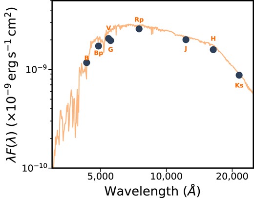
Spectral energy distribution of HIP 113103. We make use of the spectroscopic atmospheric priors and the photometric magnitudes of HIP 113103 to constrain the stellar properties simultaneous to our global modeling of the stellar and planetary parameters.
In addition, HIP 113103 also received 1 yr of observations from the Wide Angle Search for Planets (WASP) Consortium (Pollacco et al. 2006) with the Southern SuperWASP facility, located at the Sutherland Station of the SAAO. The SuperWASP observatory consists of eight Canon 200-mm f/1.8 telephoto lenses, yielding a |$7.8^\circ \, \times \, 7.8^\circ$| field of view each over a |$2\mathrm{K}\, \times \, 2\mathrm{K}$| detector. SuperWASP observations of HIP 113103 spanned 2006-05-07 to 2007-11-13, yielding ∼11 000 epochs of observations. The periodogram from the SuperWASP light curves are also overplotted in Fig. 8, yielding a rotation period of 9.90 ± 0.23 d, consistent with the TESS observations more than a decade later. When combined, the TESS and WASP data sets provide a long term stable rotation period of 9.92 ± 0.23 d for HIP 113103. In addition, we make use of the measured rotational velocity vsin I⋆ and the photometric rotation period to provide a 1σ lower limit for the stellar inclination angle of I⋆ > 56° (Masuda & Winn 2020), consistent with an aligned geometry. Using |$R_{\star }=0.742\pm 0.013\, R_{\odot }$| and Prot = 9.92 ± 0.23 d, we also calculate an equatorial velocity of Veq = 3.78 ± 0.11 km s−1, which is in good agreement with our |$v\, \text{sin}\, i$| value of 3 ± 1 km s−1.
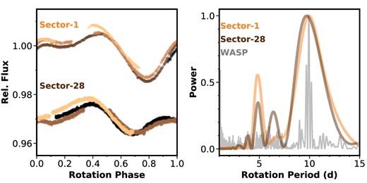
Spectral energy distribution of HIP 113103. We make use of the spectroscopic atmospheric priors and the photometric magnitudes of HIP 113103 to constrain the stellar properties simultaneous to our global modeling of the stellar and planetary parameters.HIP 113103 exhibits significant spot-induced rotational variability in its light curves. Left: TESS light curves from Sectors 1 and 28 folded to the rotation period of HIP 113103; each rotation cycle is plotted in a progressively lighter shade. The sectors are separated by an arbitrary vertical offset. HIP 113103 maintains a constant rotation period over the multiyear observations obtained by TESS. Right: Autocorrelation periodograms of the TESS and SuperWASP light curves of HIP 113103, showing a consistent peak at 10.0 d over the course of more than 10 yr.
The rotation period of HIP 113103 is consistent with an adolescent K dwarf. We adopt the rotation sequence interpolation presented by Bouma et al. (2023), and derive a rotation-based age of |$470_{-110}^{+170}$| Myr at 1σ significance. Similarly, based on the rotation age relationship from Mamajek & Hillenbrand (2008), the 1σ age range for HIP 113103 is 380–510 Myr. However, gyrochronology is particularly insecure in estimating the ages of single K dwarfs. The spins of these stars may stall within the first billion years, and many around giga-year clusters exhibit similar rotation periods (e.g. Meibom, Mathieu & Stassun 2009; Agüeros et al. 2018; Douglas et al. 2019). Angus et al. (2015) accounts for a larger spread in the spin-down dispersion of low mass stars, and the relationship they provide yields a 1σ age range of 200–2000 Myr for HIP 113103. HIP 113103 lacks spectroscopic features, such as Li 6708 Å absorption and significant Calcium ii H&K emission that are usually indicative of youth, as is expected for K dwarfs older than ∼300 million yr (Fig. 7). The Calcium ii H&K derived index |$\log R^{\prime }_\mathrm{HK} = -4.69\pm 0.05$| corresponds to an age of |$1.9_{-0.5}^{+0.7}$| Gyr, consistent with the rotational derived age estimate. In addition, the isochrone modelling also provides a loose age constraint of 5 ± 2 Gyr at the 1σ level. We find no evidence that HIP 113103 is kinematically associated with comoving stars via the comove package (Tofflemire et al. 2021).2 It is therefore difficult to confirm the suspected youth of HIP 113103.
5 INVESTIGATING FALSE POSITIVE SCENARIOS
When identifying a new planetary system, it is important to carefully consider the possibilities of astrophysical and instrumental false positives.
When analysing beyond the TESS observations, HIP 113103 b and HIP 113103 c are detected with high significance on multiple instruments, yielding consistent transit depth and duration and thus sufficiently ruling out the scenario that the transit signals result from instrument false alarms of the TESS spacecraft.
We use the following steps to rule out various astrophysical false positive scenarios. We can determine that either HIP 113103 b or HIP 113103 c are not eclipsing binaries around HIP 113103 using radial velocity observations taken with CHIRON as outlined in Section 2.4. There were no detections of significant radial velocity variations at the 20 m s−1 level, ruling out stellar mass objects at the orbital period of the transit signals.
We then follow Seager & Mallén-Ornelas (2003) to use the transit shapes to constrain the probability that the transit signals were mimicked by a binary system blended with the HIP 113103. The maximum magnitude of an eclipsing binary that can produce a transit with similar shape can be estimated by
where t12 represents the ingress duration, and t13 represent the time between the first and the third contact of the transit.
We model the transit shape of both planets independently using the TESS and CHEOPS light curves without putting any priors on the stellar parameters. We found the 3σ Tmag upper limit of any background stars capable of producing these transit signals are 13 (ΔM < 4.23 mag) and 12 (ΔM < 3.06 mag) for HIP 113103 b and HIP 113103 c, respectively.
We rule out an hierarchical binary system associated with HIP 113103, satisfying the above criteria. Neither CHIRON nor the HARPS observations (Section 2.4) detected secondary spectra lines, indicating no slow rotating, spectroscopic blended companions at ΔM < 4 (Zhou et al. 2021).
For non-associated background binaries, we can use the Gaia DR3 catalogue to rule out stars brighter than our magnitude limit up to 1 arcmin away from HIP 113103. There are no stars within 20 arcsec of HIP 113 103 based on Gaia DR3 catalogue. We estimate the density of stars brighter than our magnitude limit within 1 arcmin of HIP 113103 (which may be unresolved) by following the procedure described in Zhou et al. (2021). We found that the chance of finding a random star in the direction of HIP 113103 with ΔM < 4.2 and ΔM < 3 are 3 × 10⁻⁵ and 1 × 10⁻⁵.
Taken together, the combined observations that the system hosts multiple planets, the box-shaped transits, and the lack of additional stars in the spectra and background give us high confidence that HIP 113103 b and HIP 113103 c are genuine planets.
We also conducted a statistical validation on the TESS observations using the triceratops package (Giacalone et al. 2021), the false positive probability (FPP) yielded 0.052 for HIP 113103 b and 0.026 for HIP 113103 c. The Nearby Star FPP (NFPP) for both planets is 0. The main contributor to the FPP is the scenario that a transiting planet with the same period is around an unresolved secondary star (known as STP). We have high confidence that CHIRON and HARPS spectra can rule out secondary stars in the same system within |$\Delta$|mag of 4, which is the magnitude limit to cause a transit given the transit shape constraints. The rest of false positive scenario have total FPP less than 1e-3, therefore we can confidently call both candidates planets.
6 RESULTS AND DISCUSSION
6.1 Planet properties
We statistically validate the planetary nature of the HIP 113103 system, with the best-fitting planetary parameters presented in Table 4. HIP 113103 b has a radius of Rp = |$1.829_{-0.067}^{+0.096}$| R⊕, placing it in the upper bound of the radius gap, a small population of planets within the radii bounds 1.5 R⊕ < Rp ≤ 2 R⊕ which may be the transition point from super-Earths to mini-Neptunes via photoevaporation-driven mass loss (Fulton et al. 2017). HIP 113103 c has a radius of Rp = |$2.40_{-0.08}^{+0.10}$| R⊕, and an equilibrium temperature of 585 ± 10 K, making it a warm mini-Neptune.
We compare the HIP 113103 system with other K stars hosting multisub-Neptune planets with Teq ≤750 K in (Fig. 9), evaluating the transmission spectroscopy metric (TSM) for each target (Kempton et al. 2018). Due to the relative brightness of HIP 113103 (V ∼10 mag) and high equilibrium temperatures, HIP 113103 b (TSM = 53) and HIP 113103 c (TSM = 68) are the second most suited system around a K star for atmosphere characterization [only succeeded by the HD 73 583 system (Barragán et al. 2022)], and therefore invaluable targets to understand how multisub-Neptune systems might evolve around K-stars. This stellar population is optimal for radial velocity due to its brightness in comparison to planets orbiting M-dwarfs (Neil & Rogers 2018; Rojas-Ayala 2023). This aids the detection of smaller planets around a stellar population that shares similar characteristics to G-stars (Howard et al. 2012). Additionally from an atmosphere analysis perspective, K-stars have had repeated success at hosting planets with absorption at the He i 10 830 Å line, a tracer associated with atmosphere evaporation (Nortmann et al. 2018; Allart et al. 2019; Guilluy et al. 2020; Fu et al. 2022). Although the TSM values for HIP 113103 b and HIP 113103 c are below the J-band priority threshold of 90 (for targets within the 1.5 R⊕ ≤ Rp ≤ 10 R⊕), the derived radii of the planets combined with their close proximity to HIP 113103, and its Gyrochronological age make it a valuable system to explore through atmosphere analysis.
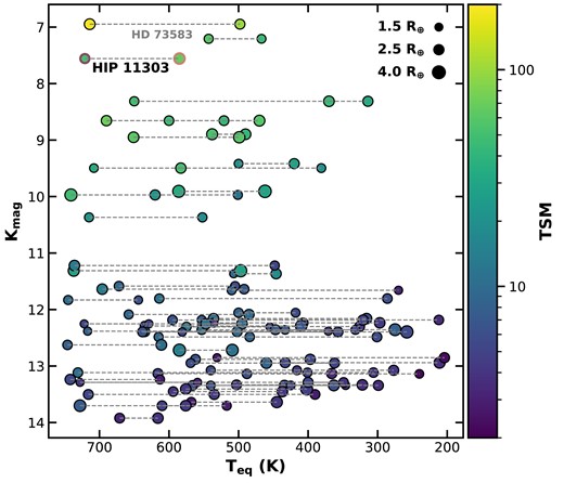
The HIP 113103 system in the context of other multiplanet systems. Specifically, we show multiplanet systems hosting two or more warm Neptunes or super-Earths with equilibrium temperature Teq ≤750 K, orbiting K stars as a function of their equilibrium temperature and K-band magnitude. The dashed lines connect each planet within the respective planetary system. The HIP 113103 system orbits one of the brightest K-dwarf host stars, and are promising candidates for follow up atmospheric observations. The colour bar illustrating the TSM for each planet places the HIP 113103 system as second highest suitable for atmosphere analysis, behind the HD 73 583 system (Barragán et al. 2022).
To estimate the mass of both planets to gauge the feasibility of future follow-up observations, we adopt the mass–radius relationship from Wolfgang et al. (2016). We estimate Mp = 5.9 ± 1.9 M⊕ for HIP 113103 b and Mp = 8.4 ± 1.9 M⊕ for HIP 113103 c. These correspond to radial velocity semi-major amplitudes of 2.34 m s−1 and 2.67 m s−1, respectively. Additional analysis using the Echelle SPectrograph for Rocky Exoplanets and Stable Spectroscopic Observations (ESPRESSO; Pepe et al. 2021) instrument on the Very Large Telescope (VLT) to understand this system in greater detail is currently underway.
6.2 Transit timing variations
We search for transit timing variations (TTVs), indicative of interactions between the two planets, or the presence of additional companions. To derive accurate transit times for each event, we perform an additional global model of the system, as per Section 3, where the transit epoch of each transit event is a free variable, and the period is held fixed. The resulting transit times are displayed in Fig. 10. We find no evidence for deviations from a linear ephemeris propagation larger than 4.5 (resp. 2.5) min (1σ scatter) for HIP 113103 b (resp. c). The mean timing uncertainty per transit is 5.7 (resp. 3.3) min, consistent with the measured scatter. We estimated the expected TTV amplitude for the system using ttvfaster (Agol & Deck 2016). Given the pair of planets has a period ratio within 10 per cent of the 2:1 mean motion resonance, we can estimate that if the planets are on modest eccentric orbits or are relatively massive, they are highly likely to exhibit TTVs with amplitudes detectable by our observations. In detail, if both planets are of Neptune mass (∼|$17\, \mathrm{ M}_{\oplus }$|), and we assume relatively low eccentricities follow a Rayleigh distribution with |$\sigma {_e}=0.06\, (\text{consequent mean eccentricity,}\, \bar{e} = 0.075)$|, the median TTV scatter for HIP 113103 b (resp. HIP 113103 c) should be on the 10 (resp. 15) min time-scale (Jurić & Tremaine 2008). If we adopt masses for both planets as per the mass–radius relationship from Wolfgang et al. (2016), ttvfaster estimates that the eccentricity of the system is most likely lower than 0.2 given the non-detection of a significant TTV signal. This puts tighter constraints on the system eccentricity compared to our global modeling. This eccentricity upper limit is derived by comparing the scatter in the transit times from ttvfaster simulations and the observed data. We first compute the 3 sigma scatter of the transit times from the data set presented in Fig. 10. We then compute the corresponding eccentricities of the systems that would produce larger transit time deviations in 95 per cent of the simulations.
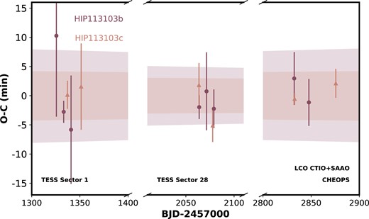
Deviations from linear transit times for individual transits of HIP 113103 b (circle markers) and HIP 113103 c (triangle markers) from all photometric observations, with each facility identified via labels along the time axis. Using our global fitted T0 values to serve as the linear baseline for HIP 113103 b and HIP 113103 c, we show that over a 4-yr period, the transit midpoint for each target does not vary beyond ∼10 min shaded regions denote the 1σ propagated transit timing uncertainties for each respective planet. Note that the individual transit times are fully consistent with the linear transit ephemeris.
6.3 Prospect for atmospheric follow-up
Systems hosting transiting small planets are optimal for understanding the radius evolution and mass-loss processes that sculpt the close-in sub-Neptune population (e.g. Owen & Campos Estrada 2020). Having planets that formed from the same protoplanetary disc and experienced the same host star XUV evolution, allows us to test photoevaporation processes by isolating the effects of insulation on mass-loss. We tested for the future prospect of atmospheric transmission spectroscopic observations for the planets in the HIP 113103 system via a set of current and upcoming space-based facilities, including the Twinkle Space Telescope (Twinkle; Stotesbury et al. 2022), HST (Kimble et al. 2008; Tsiaras et al. 2016), and JWST (Bean et al. 2018; Jakobsen et al. 2022). Twinkle is a visible to infrared (|$0.5\, \mu$|m|$- 4.5 \ \mu$|m) 0.45-m space telescope set to begin scientific operations in 2025 at a 700 km geocentric Sun-synchronous orbit.
The simulated transmission Twinkle spectra is generated for both channels (|$0.5\, \mu$|m ≤ Ch0 |$\le 2.43\, \mu$|m, |$2.43\, \mu$|m ≤ Ch1 |$\le 4.5\, \mu$|m) using the radiometric tool available on the mission’s data base Stardrive3, while the HST (WFC3 NIR G141 grism: |$1.075\, \mu$|m|$-1.7\, \mu$|m) and JWST (NIRSpec G395H grism: |$2.87\, \mu$|m |$-5.14\, \mu$|m) transmission spectra are generated using the publicly available noise simulator, pandexo (Batalha et al. 2017). The synthetic transmission spectra are processed through the retrieval framework taurex 3.0 (Al-Refaie et al. 2021), which generates an atmosphere divided into 100 evenly spaced layers across a log grid varying from 10−4 to 106 Pa. The trace gases in our models were assumed to be in chemical equilibrium and the abundances were calculated using fastchem (Stock et al. 2018). We keep the C/O ratio fixed at 0.54 (an oxygen rich atmosphere at solar abundances as discussed in Madhusudhan 2012) and assume a metallicity of |$100\, \times$| Solar for HIP 113103 b and |$10\, \times$| Solar for HIP 113103 c, aligning with previous studies that relate metallicity and low-mass planets as being inversely proportional (e.g. Fortney et al. 2013; Kreidberg et al. 2014; Charnay, Meadows & Leconte 2015). The trace gases inserted into this atmosphere included the molecular opacities of CH4 (Hill, Yurchenko & Tennyson 2013; Yurchenko & Tennyson 2014), CO (Li et al. 2015), CO2 (Rothman et al. 2010), H2O (Polyansky et al. 2018), and NH3 (Yurchenko, Barber & Tennyson 2011), with all opacities being obtained through the ExoMol (Tennyson et al. 2016) and HITRAN data bases (Gordon et al. 2016). In addition, we also implement Rayleigh scattering for all inserted molecules (Cox 2015), provide a collision induced absorption from H2–H2 (Abel et al. 2011; Fletcher, Gustafsson & Orton 2018) and H2–He interactions (Abel et al. 2012). For each instrument, we modelled both a clear atmosphere scenario (i.e. P = 106 Pa) and a uniform opaque deck scenario (i.e. grey clouds) at P = 101 Pa.
We present our simulated spectra of HIP 113103 b in Fig. 11 and HIP 113103 c in Fig. 12. Should HIP 113103 b and HIP 113103 c reflect a similar composition as our simulated spectra, we can recover a transmission spectra from 10 orbits using Twinkle (top panels; Stotesbury et al. 2022). Likewise, Figs 11 and 12 demonstrate the precision we can expect to achieve from one orbit observation using the infrared WFC3 G141 grism (middle panels) on HST (Kimble et al. 2008; Tsiaras et al. 2016) and NIRSpec G395H grism (bottom panels) on JWST (Bean et al. 2018; Jakobsen et al. 2022). We can successfully retrieve molecular species for HIP 113103 c with each instrument given a clear atmosphere (with H2O and CO2 displaying the strongest absorption). However, in the event of clouds, we would struggle to detect any signal for HIP 113103 c using Twinkle and HST instruments. Distinguishing between a clear or cloudy atmosphere on all three instruments is challenging for HIP 113103 b. An atmosphere that is in chemical disequilibrium for both targets could result in stronger absorption but would be dependent on various unknown physical parameters. Alternatively, the evolutionary path of HIP 113103 b could be the product of a migrated Water World instead of photoevaporation of a mini-Neptune (e.g. Luque & Pallé 2022); however, this scenario can only be explored in more detail after planet density measurements have been calculated. Our density estimation for HIP 113103 b of |$0.96^{+0.15}_{-0.22}$| ρ⊕ is indicative of a rocky planet, but is inferred from a mass–radius relationship and may not reflect the true bulk density of the planet. Accurate mass measurements of HIP 113103 b and HIP 113103 c are required to confirm their densities.
A synthetic atmospheric transmission spectra of HIP 113103 b, incorporating absorbing species CH4, CO, CO2, H2O, and NH3 at chemical equilibrium assuming an atmospheric metallicity of |$100\times$| Solar. The top panel illustrates the expected spectrum after 10 visits with Twinkle, the middle panel shows the simulated spectrum from a single visit with HST WFC3 with the G141 grism, and the bottom panel shows the simulated spectrum from a single visit with JWST NIRSpec G395H grism (with each instrument capturing a different wavelength range). For each facility, we have illustrated two scenarios: one where spectrum is cloud-free (106 Pa), and another with a grey cloud deck (101 Pa). The synthetic spectra for Twinkle was obtained using the radiometric tool on the Twinkle Stardrive portal, while the HST and JWST spectra were generated using pandexo.
A synthetic atmospheric transmission spectrum of HIP 113103 c, with absorbing species including CH4, CO, CO2, H2O, and NH3 in chemical equilibrium at an atmospheric metallicity of |$10\times$|Solar. Figure configuration is as per Fig. 11, with the Twinkle retrieval representing 10 visits.
7 CONCLUSION
In this paper, we confirm the existence of two sub-Neptunes, HIP 113103 b and HIP 113103 c, within |$\sim 10\%$| of 2:1 resonance around the bright K3V star HIP 113103. First identified with TESS, this system is revisited using both ground based transit observations (observed with the photometric LCO network and on the CHIRON spectrograph), as well as a space-based photometric observations of both targets within a ∼17.5-h visit using CHEOPS. Follow up TTV analysis does not reveal any additional outer companions. Our planetary parameters revealed a radius of Rp = |$1.829_{-0.067}^{+0.096}$| R⊕ for HIP 113103 b and Rp = |$2.40_{-0.08}^{+0.10}$| R⊕ for HIP 113103 c, confirming both targets reside within the mini-Neptune sub-class. For HIP 113103 b, the combination of its close proximity to HIP 113103 and its planetary radius means it resides within the radius gap, which if confirmed via mass follow up, would add an additional target a sparse sub-class of planets which are hypothesized to bridge the formation transition between super-Earths and mini-Neptunes. If HIP 113103 b is the subject of atmosphere evaporation due to its close proximity to HIP 113103, our generated retrieval plots (using the Twinkle, HST, and JWST telescopes) suggest it would be a struggle to distinguish an evolutionary gap via metallicity disparity for all three telescopes (assuming chemical equilibrium), even if there is a clear atmosphere. Ultimately, this system provides two key targets capable of atmospheric analysis within the population of mini-Neptune multiplanet systems orbiting K-stars.
ACKNOWLEDGEMENTS
We would like to acknowledge and pay respect to Australia’s Aboriginal and Torres Strait Islander peoples, who are the traditional custodians of the lands, the waterways, and the skies all across Australia. We thank Australia’s Aboriginal and Torres Strait Islander peoples for sharing and caring for the land on which we are able to learn. In particular, we pay our deepest respects to all Elders, ancestors, and descendants of the Giabal, Jarowair, and Yuggera nations, upon which the Minerva-Australis facility is situated, and analysis for this paper was undertaken. We would also like to acknowledge and pay our deepest respects to the Indigenous Elders, ancestors and descendants who are the traditional custodians of the land upon which the CTIO, SAAO, and ESO 3.6-m are situated. This includes (but may not be exclusive to) the Diaguita and Khoisan nations. GZ thanks the support of the Australian Research Council (ARC) Discovery Early Career Research Award (DECRA) programme DE210101893. CXH thanks the support of the ARC DECRA programme DE200101840. GZ and SQ thank the support of the TESS Guest Investigator Program G03007. CH thanks the support of the ARC DECRA programme DE200101840. KAC acknowledges support from the TESS mission via subaward s3449 from MIT. This research has used data from the CTIO/SMARTS 1.5-m telescope, which is operated as part of the SMARTS Consortium by RECONS. This work makes use of data from the European Space Agency (ESA) mission CHEOPS via the CHEOPS Guest Observers Program AO-3-10. This work has made use of data from the ESA mission Gaia, processed by the Gaia Data Processing and Analysis Consortium (DPAC). Funding for the DPAC has been provided by national institutions, in particular the institutions participating in the Gaia Multilateral Agreement. This work makes use of observations from the LCOGT network. Part of the LCOGT telescope time was granted by NOIRLab through the Mid-Scale Innovations Programme (MSIP). MSIP is funded by NSF. This work makes use of data from the Minerva-Australis facility. Minerva-Australis is supported by Australian Research Council LIEF Grant LE160100001, Discovery Grants DP180100972 and DP220100365, Mount Cuba Astronomical Foundation, and institutional partners University of Southern Queensland, University of New South Wales Sydney, Massachusetts Institute of Technology, Nanjing University, George Mason University, University of Louisville, University of California Riverside, University of Florida, and The University of Texas at Austin. This research has made use of the NASA Exoplanet Archive, which is operated by the California Institute of Technology, under contract with the National Aeronautics and Space Administration under the Exoplanet Exploration Programme. This work has been carried out within the framework of the NCCR PlanetS supported by the Swiss National Science Foundation under grants 51NF40182901 and 51NF40205606. Funding for the TESS mission is provided by NASA’s Science Mission directorate. We acknowledge the use of public TESS Alert data from pipelines at the TESS Science Office and at the TESS Science Processing Operations Center. This research has made use of the Exoplanet Follow-up Observation Programme (ExoFOP; DOI: 10.26134/ExoFOP5) website, which is operated by the California Institute of Technology, under contract with the National Aeronautics and Space Administration under the Exoplanet Exploration Programme. This paper includes data collected by the TESS mission, which are publicly available from the Mikulski Archive for Space Telescopes (MAST). Resources supporting this work were provided by the NASA High-End Computing (HEC) Programme through the NASA Advanced Supercomputing (NAS) Division at Ames Research Center for the production of the SPOC data products.
DATA AVAILABILITY
The data underlying this article will be shared on reasonable request to the corresponding author.
