


ABSTRACT
η Carinae is an extremely luminous and energetic colliding-wind binary. The combination of its orbit and orientation, with respect to our line of sight, enables direct investigation of the conditions and geometry of the colliding winds. We analyse optical He i 5876 and 7065 Å line profiles from the Global Jet Watch observatories covering the last 1.3 orbital periods. The sustained coverage throughout apastron reveals the distinct dynamics of the emitting versus absorbing components: the emission lines follow orbital velocities, while one of the absorption lines is detected only around apastron (0.08 < ϕ < 0.95) and exhibits velocities that deviate substantially from the orbital motion. To interpret these deviations, we conjecture that this He i absorption component is formed in the post-shock primary wind, and is only detected when our line of sight intersects with the shock cone formed by the collision of the two winds. We formulate a geometrical model for the colliding winds in terms of a hyperboloid in which the opening angle and location of its apex are parametrized in terms of the ratio of the wind momentum of the primary star to that of companion. We fit this geometrical model to the absorption velocities, finding results that are concordant with the panchromatic observations and simulations of η Carinae. The model presented here is an extremely sensitive probe of the exact geometry of the wind momentum balance of binary stars, and can be extended to probe the latitudinal dependence of mass-loss.
1 INTRODUCTION
Colliding-wind binaries are characterized by two massive stars both driving powerful stellar winds. These winds collide forming shock fronts in a cone-like shape at the surface where their wind momenta balance. In these shocks, the gas is compressed and heated, leading to the production of X-rays (Cherepashchuk 1976; Prilutskii & Usov 1976; Luo, McCray & Mac Low 1990), non-thermal emission (Pollock 1987; White & Chen 1994; Hamaguchi et al. 2018), and dust (Williams 2008). The presence of the shock cone may also modulate the ultraviolet and optical line profile variability during the binary’s orbit (Stevens 1993; Szostek, Dubus & Mcswain 2012).
η Carinae (hereafter η Car) is one of the most luminous and energetic colliding-wind binaries in the Milky Way having a luminosity of |$L=5 \times 10^6 \, \rm {L_{\odot }}$| (Davidson & Humphreys 1997) and an observed long-term brightening due to a vanishing natural coronagraph (Damineli et al. 2021; Gull et al. 2022; Pickett et al. 2022). The primary star is a luminous blue variable exhibiting one of the strongest winds on record: a mass-loss rate of |${\sim }8.5 \times 10^{-4} \, \rm {{\rm M}_{\odot }\, yr^{-1}}$| and terminal wind velocity of |${\sim }420 \, \rm {\, km \, s^{-1}}$| (Hillier et al. 2001; Groh et al. 2012; Clementel et al. 2015a).
The companion star, despite having not been observed directly, is estimated to have a mass-loss rate and terminal wind velocity of ∼(1–2)|$\times 10^{-5} \, \rm {{\rm M}_{\odot }\, yr^{-1}}$| and |${\sim }3000 \, \rm {\, km \, s^{-1}}$|, respectively. These are deduced from modelling the X-ray emission from η Car’s colliding winds (Pittard & Corcoran 2002; Okazaki et al. 2008; Parkin et al. 2011; Russell et al. 2016). Photoionization modelling of the spectral variability of η Car’s Weigelt blobs (Weigelt & Ebersberger 1986) indicated that the companion may be a hot O-star, with an effective temperature between 34 000 and 38 000 K (Verner et al. 2002; Verner, Bruhweiler & Gull 2005). However, as noted by Smith et al. (2018), the companion’s wind parameters may be more consistent with those of a hydrogen-poor Wolf–Rayet (WR) star. Smith et al. (2018) described a possible formation channel for this present-day companion via a past merger-in-a-triple scenario, and this has been shown to be tenable by the models of Hirai et al. (2021).
Whether the companion is an O-star or a WR star, it is known to generate a significant flux of helium-ionizing photons (λ < 504 Å, hν > 24.6 eV), which significantly affects the ionization structure of the system. There has been a substantial effort to map the ionization structure of helium within the central 155 au of η Car. This is because the helium lines can be used to probe the conditions within the colliding-wind interface, as has been utilized for other colliding-wind binaries such as V444 Cygni (Marchenko, Moffat & Koenigsberger 1994) and WR 140 (Williams et al. 2021).
As for η Car, there has been some speculation as to whether the He i lines are formed in the primary wind (Nielsen et al. 2007; Humphreys, Davidson & Koppelman 2008) or in the shock cone of the colliding winds (Damineli et al. 2008b). More recently, the three-dimensional radiative transfer simulations of Clementel et al. (2015a, b), taking into account the ionization structure of the primary wind and the effect of the companion’s radiation, resulted in detailed helium ionization maps for η Car. Since then, spectro-interferometric observations, with the infrared K-band beam-combiner GRAVITY at the Very Large Telescope Interferometer (VLTI), have enabled milliarcsecond resolution observations of the He i 2s–2p (2.0587 μm) line transition (GRAVITY Collaboration 2018) and these results show good agreement with the helium ionization maps of Clementel et al. (2015a). In combination with these helium ionization maps, the estimated orbit (Damineli et al. 2000; Grant, Blundell & Matthews 2020; Grant & Blundell 2022) and orientation (Madura et al. 2012; Teodoro et al. 2016) mean that our line of sight intercepts the shock cone, providing an exceptional opportunity to study the conditions and geometry of η Car’s colliding winds.
In this study, we investigate the geometry of η Car’s colliding winds through time-series spectroscopic observations of the optical He i line profiles. In Section 2, we present observations from the Global Jet Watch’s campaign on η Car. We show that at different orbital phases the He i absorption varies, exhibiting distinct components at periastron and apastron. In Section 3, we employ multi-Gaussian fits to track the dynamics of these He i components, revealing that one of the absorption component’s velocities deviates substantially from the expected orbital motion. We then describe a geometrical model of the colliding winds, cognisant of the known helium ionization maps, from which we simulate the He i absorption velocities. We fit this model to the Global Jet Watch data and tabulate the inferred parameters. In Section 4, we discuss the latitudinal dependence and assumptions of this geometrical model. Finally, in Section 5 we summarize our findings.
2 OBSERVATIONS
The Global Jet Watch is a network of five remotely controlled observatories separated in longitude to enable round-the-clock observing. The observatories are situated in South Africa, India, on the west and east coasts of Australia, and Chile. Each observatory has a fibre-fed spectrograph, and a 0.5 m telescope, that collects mid-resolution (|$R \, {\sim }\, 4000$|) optical data in the wavelength range ∼5800–8400 Å. The spectra are reduced by a bespoke data reduction pipeline that includes dark correction, flat-field correction, and wavelength calibration derived from thorium–krypton frames. Full details of the observatories and instruments will be described in Blundell et al. (in preparation) and Lee et al. (in preparation), respectively.
The spectra have their telluric absorption corrected for using telfit (Gullikson, Dodson-Robinson & Kraus 2014). This software is a wrapper to the line-by-line radiative transfer model (LBLRTM; Clough et al. 2005). LBLRTM is a well-tested and reliable radiative transfer model that is both accurate and efficient for modelling telluric absorption. For each spectrum, telfit is used to produce a model of the tellurics by fitting the pressure, temperature, humidity, and resolution to the spectral data. Other important observation parameters (latitude, altitude, zenith angle) are set from the observatory metadata. During the fitting process, telfit is given specific wavelength regions to ignore from the data that correspond to strong emission lines in the data. The resulting model telluric spectra are then subtracted from the η Car spectra.
The Global Jet Watch observing campaign of η Car began in early 2014 and since has amounted 5858 spectra across 1.3 orbital periods (2630 d), spanning the 2014 and 2020 periastra. These observations have exposure times ranging from 1 to 300 s to capture both the H α and He i lines at acceptable signal-to-noise ratios while avoiding saturation. Pertinent to this study, the observations are densely time sampled throughout the orbital period, not just at periastron, and thereby provide excellent coverage of η Car’s apastron. An example spectrum is displayed in Fig. 1.
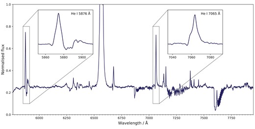
Example spectrum of η Car taken from the Global Jet Watch observatory in Western Australia. Here, we show the data prior to telluric correction but with the continuum removed. Inset panels display the two He i lines analysed in this work.
2.1 The He i line profiles
In this paper, we focus our analysis on the He i line profiles. As such, we select the 3554 Global Jet Watch spectra having exposure times of at least 100 s. These spectra are normalized by their local continuum and are barycentric corrected to the Solar system using the barycorrpy package (Kanodia & Wright 2018). To further improve the signal-to-noise ratio, especially for the weaker blueshifted absorption components, we median stack the spectra into orbital phase bins of width 0.01. These phase bins are computed according to the period, P = 2022.7 d, of Damineli et al. (2008a), and the time of periastron, T0 = 2454 850.1 (JD), of Grant & Blundell (2022). The He i lines have signal-to-noise ratios of ∼100 at the continuum level and of ∼200–300 at the peak of the lines.
Initial analysis of the three He i lines in the Global Jet Watch spectra shows that both lines at 5876 and 6678 Å suffer blending from other species. As has been previously noted by Richardson et al. (2015), the red wing of the He i 5876 Å line is blended with the complex Na i D doublet, and the blue wing of the He i 6678 Å line is blended with a [Ni ii] line. As a result, we restrict our analysis to the unencumbered He i 7065 Å line, as well as the blue wing of the He i 5876 Å line. From these lines, we can obtain clear dynamical information from the blueshifted absorption components from both lines, and from the emission component of the He i 7065 Å line.
In Figs 2 and 3, we plot all of our 0.01 phase-binned spectra for the He i 5876 and 7065 Å lines, respectively. Alongside these spectra, we also present the data binned further into bins of 0.1 phase, to further elucidate the changing morphology of the emitting and absorbing components throughout η Car’s orbit. In terms of emission, we observe the expected variability: a low-excitation event at periastron in which the narrow emission component disappears and the bulk velocity of the emission region shifts violently with the extremely eccentric periastron passage (Groh & Damineli 2004; Nielsen et al. 2007; Humphreys et al. 2008; Damineli et al. 2008a, b; Mehner et al. 2010, 2012; Richardson et al. 2015). As for the blueshifted absorption, we discern two distinct components in these line profiles. At periastron, we observe strong absorption, at a velocity of |${\sim }{-500}\, \rm {\, km \, s^{-1}}{}$|, which has been detected and analysed previously (e.g. Richardson et al. 2015). However, a second component, found at slower negative velocities, is detected only either side of periastron. In Figs 2 and 3, this behaviour is apparent, where the line profiles corresponding to phases around apastron clearly show this absorption component. We measure this second component to disappear at ϕ = 0.95 and reappear at ϕ = 0.08.
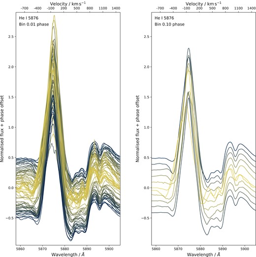
He i 5876 Å spectral line profiles binned into 0.01 phase bins (left) and 0.10 phase bins (right). The continuum has been removed and the y-offset corresponds to the orbital phase. The profiles are colour-coded with brighter yellow indicating the proximity to η Car’s periastron (phase offset = zero). The corresponding velocities are shown on the top x-axes.
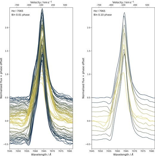
The same as Fig. 2 but for the He i 7065 Å spectral line profiles.
2.2 He i absorption dynamics
To extract velocities from the He i 5876 and 7065 Å lines, we employ multi-Gaussian fitting to decompose the complex line profiles into their constituent dynamical components. Following Nielsen et al. (2007), we construct a multi-Gaussian template comprised of four Gaussians to model the main emission, two negative Gaussians to model the blue-shifted absorption, and a low-amplitude broad Gaussian to model the extended wings of the profile. For the He i 5876 Å line, we only use three Gaussians to model the emission, because, as noted in Section 2.1, we only consider the blue wing (|$\lambda \lt 5875\, {{\mathring{\rm A}}}$|) due to the impact of Na absorption at longer wavelengths.
The Gaussian parameters are optimized using a trust region reflective algorithm (Branch, Coleman & Li 1999; Jones, Oliphant & Peterson 2001) that minimizes the sum of squares between the multi-Gaussian model and the observed spectral line profiles. We fit both the He i 5876 and 7065 Å lines simultaneously, and link the velocity of the main absorption component between each of the two lines. By linking the absorption velocities in this way, we constrain the absorption dynamics to represent the information of both lines, leading to a more robust picture of the He i dynamics. These choices are validated by a our multi-Gaussian template producing consistently good fits across all of the spectra. Further checks are made to assess the goodness of fit, such as testing whether the normalized residuals show a normal distribution as suggested by Riener et al. (2019). Example multi-Gaussian fits are displayed in Fig. 4. Here, the absorption components, shown in orange, have their velocity linked during the simultaneous fitting of the He i 5876 and 7065 Å lines as described above.
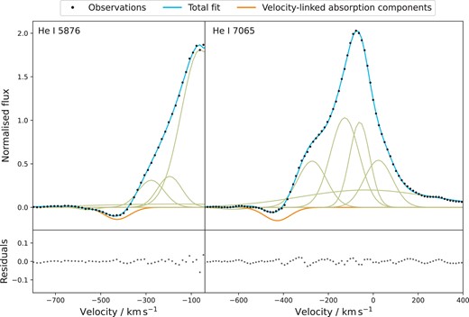
Example simultaneous multi-Gaussian fitting of the He i 5876 and 7065 Å spectral line profiles at ϕ = 0.61. The orange absorption component has its velocity linked between the two lines. The light blue line is the total model. The bottom of each panel shows the residuals of each fit.
After fitting the line profiles, we examine the extracted velocities. For the bulk velocity of η Car’s wind emission region, we take the weighted mean of the He i 7065 Å line’s four main emission components (centroid wavelength of each Gaussian weighted by its area; see Blundell, Bowler & Schmidtobreick 2007; Grant et al. 2020). For the absorption velocities, we take the centroid of the velocity-linked absorption component. We plot these velocities in Fig. 5 and tabulate them in Table A1. Note that the absorption velocities are not present near to periastron as this component is not detected at these times, as was discussed in Section 2.1.
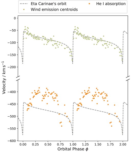
Emission (green, top) and absorption (orange, bottom) velocities extracted from the multi-Gaussian fits to the He i spectral lines. η Car’s radial velocity curve estimated by Grant & Blundell (2022) is superimposed for comparison (dashed lines + offsets). The absorption represents the velocity-linked absorption component shown in orange in Fig. 4.
In Fig. 5, it is clear that the emission and absorption components encode dynamical information from distinct regions of η Car. The emission velocities show similar dynamics to the line-of-sight orbital motion of the system (dashed line), as predicted by the models of Grant et al. (2020) and Grant & Blundell (2022). However, the absorption velocities show apparent deviations from the orbital motion. These deviations are most prominent during apastron as the velocities arc upwards to slower values. Understanding these absorption dynamics will now form the focus of the remainder of this study.
3 TRACING THE COLLIDING WINDS
In this section, we formulate a physical model for interpreting the behaviour of the He i absorption and apply this model to the Global Jet Watch observations.
3.1 The line formation regions of helium
In order to model the dynamics of the He i absorption, we must first consider the helium line formation regions in η Car. The companion is known to be a source of helium ionizing photons (Verner et al. 2002, 2005; Hillier et al. 2006) that significantly affects the helium ionization structure of the system; and hence, any quantities deduced from these lines.
In Fig. 6, we reproduce the schematic of the helium ionization map from GRAVITY Collaboration (2018, their fig. 14), which is based on the simulations of Clementel et al. (2015a, their figs 7 and 8) for the central 155 au of η Car. In this schematic, we colour each region based on its helium ionization level: |$\rm {He}^{0+}$| (blue), |$\rm {He}^{1+}$| (yellow), and |$\rm {He}^{2+}$| (grey). The primary wind is predominately |$\rm {He}^{0+}$|, except for two |$\rm {He}^{1+}$| regions. The first is the small volume surrounding the primary star that is ionized by radiation directly from the primary star. The second is the region adjacent to the apex of the colliding wind, which is ionized by radiation from the companion. Here, we see how only gas sufficiently close to the shock cone is able to be reached by the companion’s ionizing flux. In addition to these two regions, |$\rm {He}^{1+}$| also exists in the post-shock primary wind in the walls of the shock cone cavity, denoted by the dashed lines in Fig. 6, and throughout most of the pre-shock companion wind. The post-shock companion wind is solely comprised of |$\rm {He}^{2+}$| owing to collisional ionization caused by the high temperature (T > 106 K) of the shock-heated gas.
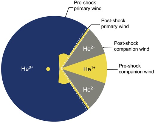
Helium ionization schematic of η Car: |$\rm {He}^{0+}$| (blue), |$\rm {He}^{1+}$| (yellow), and |$\rm {He}^{2+}$| (grey). The radius of the blue region is 155 au and the dashed lines represent the region of the post-shock primary wind formed in the interface of the colliding winds. This plot is reproduced from GRAVITY Collaboration (2018), which itself was based on the simulations of Clementel et al. (2015a) for apastron.
We are primarily concerned with the |$\rm {He}^{1+}$| regions of Fig. 6, since the observed optical He i lines are indirect consequences of recombination into the highly energetic top levels of these lines. In particular, following Damineli et al. (2008b), Clementel et al. (2015a), and GRAVITY Collaboration (2018), we presuppose that the He i absorption is formed principally in the post-shock primary wind.
3.2 A geometrical model for the colliding winds
There exist certain combinations of system orientations and colliding-wind balances in which the shock cone intersects our line of sight to the primary star. If the He i absorption is formed in the post-shock primary wind, along the walls of the shock cone, then this absorption will trace the geometry of the colliding winds as the shock cone swings across our line of sight. The dynamical information imprinted at the site of the absorption corresponds to the post-shock primary wind velocities projected on to our line of sight. This results in faster velocities the more parallel the shock cone wall is to our line of sight. Qualitatively, for orientations favoured by most investigators, with the shock cone on our side of the system during apastron, this leads to absorption velocities that appear fast as the line of sight first enters the shock cone, shortly after periastron, followed by a progressive slowing as the line of sight traces across to the centre of the shock cone at apastron. The process is then reversed as the line of sight traces out to the other side of the shock cone, the absorption velocities becoming faster, until the line of sight exits the shock cone altogether. This description mirrors the dynamical behaviour of the He i absorption found in Section 2.2 and so we pursue this line of thinking by formulating a geometric model of the colliding winds.
We begin the description of our geometric model by considering the wind momentum balance. Along the line of centres of the two stars, the wind momentum ratio is defined as
where |$\dot{M}$| is the mass-loss rate, v∞ is the terminal velocity of the wind, and the subscripts 1 and 2 correspond to the primary and companion stars, respectively. Using equation (1), the apex of the contact discontinuity occurs at
where r1 is the distance from the primary star to the contact discontinuity and D is the total separation of the two stars (Stevens, Blondin & Pollock 1992). This expression assumes that the winds collide at their terminal velocities which is valid for most of the apastron passage of η Car. The balance of ram pressures when the stars have uneven wind strengths leads to a cone-like shape for the contact discontinuity, with the asymptotic half-opening angle of this shock cone, θ, being the fundamental descriptor. Previous hydrodynamic simulations by Madura et al. (2013) found that for η Car this θ was consistent with the analytical formula of Canto, Raga & Wilkin (1996):
Given analytical expressions for the colliding wind apex’s location and asymptotic opening angle, we elect to use a hyperboloid as the geometric surface for the contact discontinuity. A hyperboloid of one sheet, orientated such that the apex and opening are along the x-axis, has the following equation:
where a = r1 sets the distance from the primary star, situated at the origin, to the apex, b = a tan θ sets the asymptotic half-opening angle in the x–y plane, and c = a tan θ sets the asymptotic half-opening angle in the x–z plane. In this way, we have included the flexibility to alter the wind momentum balance in both the equatorial and polar directions (see the model exploration in Figs 7 and 10 and the discussion in Section 4), although for the main model fitting we set both these values to be the same. A hyperboloid is a natural choice owing to its qualitative agreement with hydrodynamic models, and the ease with which the surface can encode the location and angles of the colliding winds.
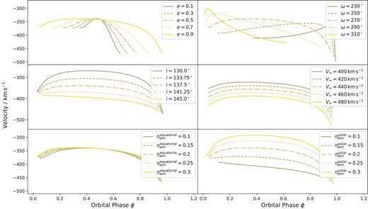
Exploration of our geometrical model for the colliding winds of η Car for various parameter combinations. Only one parameter is varied per panel, see the text for details.
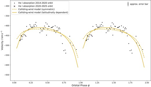
Best fit of our geometrical model for the colliding winds of η Car to the He i absorption velocities. One orbital period has been duplicated. The uncertainties on the velocity data are estimated at |$11 \, \rm {\, km \, s^{-1}}{}$|.
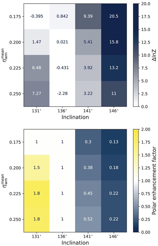
Bayesian analysis grid of model inferences based on varying the inclination and mean wind momentum ratio, |$\eta _{\rm {wm}}^{\rm {mean}}$|, of the polar and equatorial components. The top panel shows the Bayes factor comparing the evidence for the latitudinally dependent model versus the spherically symmetric model. The bottom panel shows the polar enhancement factor of the wind, defined as |$1/(\eta _{\rm {wm}}^{\rm {polar}}/\eta _{\rm {wm}}^{\rm {equatorial}})$|, for the statistically preferred model.
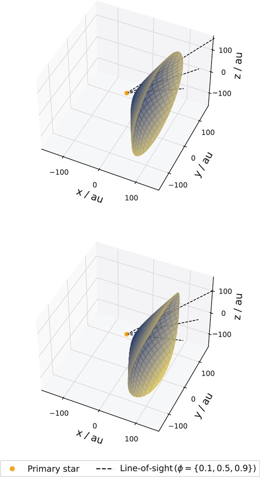
Three-dimensional renderings of the hyperboloid surfaces from our geometric models. The models are shown in the rotated frame of reference with the primary star at the origin. The dashed lines show the line of sight at three different phases: 0.1, 0.5, 0.9. Top panel: the best-fitting model from Section 3.2 for a spherically symmetric wind with i = 137.5° and ηwm = 0.20. Bottom panel: an example model from Section 4.1 for a polar enhanced wind with i = 131°, |$\eta _{\rm {wm}}^{\rm {equatorial}} = 0.22$|, and |$\eta _{\rm {wm}}^{\rm {polar}} = 0.12$|.
To synthesize the absorption velocities of the post-shock primary wind of η Car, we work in the rotated frame of reference, which has the line of centres of the two stars fixed along the x-axis, and the primary star at the origin. We compute the separation of the stars at each epoch of an orbital period and from this set the hyperboloid geometry after inputting the wind momentum ratio. Our line of sight to the primary star is then computed in this rotated frame and we can solve for the intersection, if any, between it and the hyperboloid, named as point Pint. At Pint, we compute the angle between the tangent plane to the hyperboloid and our line of sight, ϕ, in order to project the shocked gas velocities on to our line of sight.
The final absorption velocities in the post-shock primary wind, vabsor(t), as a function of time, t, are
where
In these equations, vwind is the velocity of the primary wind just prior to being shocked at point, Pint, vkep is the Keplerian velocity of the primary star projected on to the line of sight, and γ is the systemic velocity along our line of sight. The sum total of equation (6) is the velocity of the pre-shock gas in the observer’s frame of reference. Equation (5) simply projects the pre-shock velocities, first along the shock cone, and then second, on to our line of sight. The angles of these projections are both ϕ as our line of sight is co-linear with the outflowing pre-shock wind in our line of sight. We also choose to calculate vwind from the standard β-law as first derived by Castor, Abbot & Klein (1975) for line-driven winds and we set β = 1. However, we find using the terminal velocity of the wind does not affect our results by more than a few |$\, \rm {\, km \, s^{-1}}$|, because at times near to apastron the intersection point is far from the primary star.
Having described a geometrical model for the colliding winds of η Car, we now look at how the parameters that go into this model change the predicted absorption velocities. The complete parameter set is displayed in Table 1: the orbital period, P, time of periastron, T0, eccentricity, e, primary star’s semi-amplitude, k1, systemic velocity along our line of sight, γ, wind momentum ratio, ηwm, primary wind terminal velocity, v∞,1, inclination, i, and argument of periastron, ω. In addition to these tabulated parameters, we also require a value for the mass of the primary star, m1 in order to calculate the size of the semimajor axis via the mass function and Kepler’s third law. We set |$m_1=100 \, \rm {{\rm M}_{\odot }}$| that results in a semimajor axis of 17.8 au, but tests show that this choice is arbitrary for our model. The semimajor axis simply rescales the system, having a negligible impact on the absorption velocities, much like the β-law parametrization mentioned above. Consequently, we leave this parameter fixed and out of the tabulated list of key parameters in Table 1.
Parameters used in the geometrical model for the colliding winds of η Car. ‘This work’ indicates the parameters found in the best-fitting symmetric model shown in Fig. 8.
| Model parameters | Value | Reference |
|---|---|---|
| Orbital elements | ||
| P (d) | 2022.7 | Damineli et al. (2008a) |
| T0 (JD) | 2454850.1 | Grant & Blundell (2022) |
| e | 0.90 | Grant & Blundell (2022) |
| k1|$(\rm {\, km \, s^{-1}})$| | 66.8 | Grant & Blundell (2022) |
| γ |$(\rm {\, km \, s^{-1}})$| | −8.1 | Smith (2004) |
| Wind parameters | ||
| ηwm | 0.2 | Pittard & Corcoran (2002) |
| v∞,1|$[\, \rm {\, km \, s^{-1}}]$| | 509 | This work |
| Line-of-sight parameters | ||
| i (°) | 137.5 | Madura et al. (2012) |
| ω (°) | 271 | This work |
In Fig. 7, we explore the dependence of the predicted absorption velocities on the model parameters. In each panel, we vary one parameter and fix all of the others. The fixed set is e = 0.9, |$k_1 = 66.8 \, \rm {\, km \, s^{-1}}$|, |$\gamma =0 \, \rm {\, km \, s^{-1}}$|, |$v_{\infty , 1} = 420 \, \rm {\, km \, s^{-1}}$|, i = 137.5°, and ω = 270°. We further subdivide the wind momentum ratio into its equatorial and polar components, |$\eta _{\rm {wm}}^{\rm {equatorial}} = 0.2$| and |$\eta _{\rm {wm}}^{\rm {polar}} = 0.2$|. We start with the top-left panel where we examine the role of the eccentricity. Here, we find the resulting absorption velocities depend strongly on this parameter. The higher the eccentricity, the sooner our line of sight intersects with the shock cone after periastron, and the longer we trace the velocities as the shock cone sweeps more slowly across our line of sight at apastron. In the top-right panel and the middle-left panels, we vary the argument of periastron and inclination respectively. Here, we find the model is very sensitive to changes in our line of sight. The argument of periastron shifts the orbital phase at which the slowest velocities (largest projection angles) occur. The inclination changes the overall range of velocities predicted, and to a lesser extent the timing of the start and end of the intersection. This can be interpreted as lower inclinations tracing a line through the centre of the shock cone, intersecting it at a variety of angles. However, for higher inclinations the intersection angles remain small throughout, and so the projected velocities do not change much over the orbit. In the middle-right panel, we see how the velocity of the primary wind only serves to shift all of the absorption velocities to slower or faster values.
In the bottom panels of Fig. 7, we test how the wind momentum ratio affects the predicted absorption velocities of our model. In the bottom-left panel, we vary the equatorial ratio and find the model is largely insensitive to this parameter, except for some minor changes to the timing and velocities at the start and end of the intersection. This is the case because, with an inclination set at 137.5°, we trace through the shock cone high above the equatorial plane where the projected angles depend mainly on the polar ratio, as is seen in the bottom-right panel. In the bottom-right panel, we find that as the wind momentum ratio increases, meaning the companion star has a more equally balanced wind, the shock cone opening angle increases and the absorption velocities span a larger range. Conversely, for smaller wind momentum ratios our line of sight only just intersects with the cone as it becomes more closed, maintaining faster and more even velocities throughout the orbit. Once the wind momentum ratio becomes sufficiently small, there will be no intersection at any time; however, this is heavily dependent on the inclination angle as can be seen by comparing their influence on the resulting model in their respective panels. For spherically symmetric outflows, we lock the equatorial and polar wind momentum ratios together and the model dependence is the sum of the effects in these two bottom panels.
Next, we fit our model to the He i absorption velocities extracted in Section 2.2. We fix the orbital elements to literature values: P = 2022.7 d (Damineli et al. 2008a); T0 = 2454850.1 (JD), e = 0.90, and |$k_1=66.8 \, \rm {\, km \, s^{-1}}$| (Grant & Blundell 2022); and |$\gamma =-8.1 \, \rm {\, km \, s^{-1}}$| (Smith 2004). For the inclination, we use a value of i = 137.5°, the central value in the range estimated from models of the [Fe iii] emission (Madura et al. 2012), and for the wind momentum ratio we use a value of ηwm = 0.2, the value estimated from the duration of the X-ray light-curve minimum (Pittard & Corcoran 2002). For the model fitting in this section, we assume a spherically symmetric wind balance. Finally, parameters v∞,1 and ω are left free to be optimized. A summary of this parametrization is detailed in Table 1.
The model is optimized using the Levenberg–Marquardt algorithm (Moré 1978; Jones et al. 2001) to find the least-squares solution. We find that the best-fitting values for our free parameters are |$v_{\infty , 1} = 509 \, \rm {\, km \, s^{-1}}$| and ω = 271°. We display this result in Fig. 8. Additionally, we render the hyperboloid corresponding to this best-fitting solution in the top panel of Fig. 10. The model produces good fits to the data, showing the correct velocity trends as well as the correct timing of the entry (absorption first detected after periastron) and exit (absorption no longer detected this orbital cycle) of our line of sight through the shock cone. Although we note that there are several data points at phases 0.72 < ϕ < 0.78 that show faster velocities than those that can be produced by the best-fitting model. We tested the model fitting excluding these data and find the results are not sensitive to these four data points.
4 DISCUSSION
We have presented a geometrical model for the colliding winds of η Car. The fit of our model to the He i absorption velocities shows good agreement. Moreover, the parameters input into the model are concordant with the other panchromatic observations and modelling of η Car. This includes direct agreement between the helium ionization simulations (Clementel et al. 2015a), VLTI/GRAVITY observations of He i 2.0587 μm, models of the X-ray light curve (Pittard & Corcoran 2002), three-dimensional hydrodynamic simulations (Okazaki et al. 2008), Hubble Space Telescope (HST) observations with the Space Telescope Imaging Spectrograph (STIS) of [Fe iii] (Madura et al. 2012), Gemini observations with the Gemini Multi-Object Spectrograph (GMOS) of the Balmer lines (Grant et al. 2020; Grant & Blundell 2022), and now also the Global Jet Watch observations of He i 5876 and 7065 Å. This prevailing view of η Car’s fundamental parameters builds confidence in our understanding of the system: a highly eccentric colliding-wind binary oriented with the companion on the observer’s side of the system during apastron. In the remainder of this section, we consider further details of our model within the constraints of this view of η Car.
4.1 Bayesian evidence of a latitudinally dependent wind
During the model fitting undertaken in Section 3.2, we assumed spherical symmetry in the colliding winds, locking the wind momentum ratio to identical values in both the x–y and x–z planes. However, as was shown in the exploration of the model parameters in Fig. 7, specifically the middle-left and bottom-right panels, the inclination and wind momentum ratio in the polar direction are severely degenerate. In other words, the projected angles between our line of sight and the shock cone can be held constant by simultaneously decreasing the inclination of the viewing angle and decreasing the polar wind momentum ratio. Consequently, any deductions made about the wind momentum ratio rely on the inclination value, and the inclination for η Car has only been constrained to within a window of ∼20° (Madura et al. 2012; Teodoro et al. 2016).
To investigate how this may affect our results, we run some further tests. We perform Bayesian inference, using the same geometrical model as used in Section 3.2, but for a 4-by-4 grid of varying inclination and mean wind momentum ratio. The inclinations span a similar range to those found by Madura et al. (2012) and Teodoro et al. (2016) from 131° to 146°. The mean wind momentum ratios span a small range centred on the value resulting from analysis of the X-ray light curve (Pittard & Corcoran 2002) from 0.175 to 0.250. In this way, we assess how the inferred latitudinal dependence of the wind momentum ratio depends on the inclination constraints.
We run the grid for both the spherically symmetric wind model and a latitudinally dependent wind model, now allowing the polar wind momentum ratio to vary. We parametrize this latitudinally dependent model in terms of |$\eta _{\rm {wm}}^{\rm {polar}}$|, the polar wind momentum ratio, and |$\eta _{\rm {wm}}^{\rm {mean}}$|, the mean wind momentum ratio of the polar and equatorial components. The equatorial wind momentum ratio is defined as |$\eta _{\rm {wm}}^{\rm {equatorial}} = 2 \eta _{\rm {wm}}^{\rm {mean}}-\eta _{\rm {wm}}^{\rm {polar}}$|. This parametrization ensures that the latitudinally dependent model remains consistent with the X-ray light-curve observations of Pittard & Corcoran (2002). A full list of parameters and their priors is given in Table 2.
Bayesian priors corresponding to analysis in Section 4.1. All parameters listed are given a prior that follows a normal distribution, |$\mathcal {N}(\mu , \sigma)$|. The inclination priors take on a grid of distributions.
| Model parameters | Prior |$\mathcal {N}(\mu)$| | Prior |$\mathcal {N}(\sigma)$| |
|---|---|---|
| Orbital elements | ||
| e | 0.90 | 0.01 |
| k1|$(\rm {\, km \, s^{-1}})$| | 66.8 | 4.25 |
| Wind parameters | ||
| |$\eta _{\rm {wm}}^{\rm {mean}}$| | {0.175, 0.20, 0.225, 0.25} | Fixed |
| |$\eta _{\rm {wm}}^{\rm {polar}}$| | 0.2 | 0.05 |
| v∞,1|$(\rm {\, km \, s^{-1}})$| | 500 | 30 |
| Line-of-sight parameters | ||
| i (°) | {131, 136, 141, 146} | Fixed |
| ω (°) | 270 | 20 |
We use the nested sampling code dynesty (Speagle 2020) to infer the posterior parameter distributions and model evidence (or marginalized likelihood), Z, for both the spherical and latitudinally dependent models at each point in the grid. We use the Bayes factor, Δln Z = ln ZLD − ln ZSS, to select the statistically preferred model, where ZSS and ZLD are the model pieces of evidence for the spherically symmetric and latitudinally dependent models, respectively. For grid points where Δln Z > 1.15, we determine there to be substantial evidence (Kass & Raftery 1995) for the latitudinally dependent model and we infer different wind momentum ratios for the equatorial and polar directions. For Δln Z ≤ 1.15, we infer the wind momentum ratio to be spherically symmetric.
The grid of results is presented in Fig. 9. The top panel shows the Bayes factor results and we find that many of the grid points do show statistical evidence for a latitudinal wind. In the bottom panel, we show the corresponding polar enhancement factor of the wind, defined as |$1/(\eta _{\rm {wm}}^{\rm {polar}}/\eta _{\rm {wm}}^{\rm {equatorial}})$|. For grid points that have spherically symmetric models preferred, the polar and equatorial wind momentum ratios are equal and the polar enhancement equals one. For those grid points with latitudinally dependent models, we find that the wind momentum ratios bifurcate based on the inclination constraints. The polar wind momentum ratio is lower (higher) when the inclination is lower (higher). This means that the primary wind is polar enhanced for inclinations <136° and equatorially enhanced for inclination >136°, as shown in Fig. 9. Additionally, as the mean wind momentum ratio increases, the polar wind becomes stronger relative to the equatorial wind.
The model run with an inclination of 131° and |$\eta _{\rm {wm}}^{\rm {mean}} = 0.20$| is particularly interesting as this scenario leads to |$\eta _{\rm {wm}}^{\rm {polar}} = 0.16$| and |$\eta _{\rm {wm}}^{\rm {equatorial}} = 0.24$|. This implies that η Car’s primary star may have a mass-loss rate of |$1.1 \times 10^{-3}$| and |$7.1 \times 10^{-4} \, \rm {{\rm M}_{\odot }\, yr^{-1}}$| in the polar and equatorial directions, respectively. This stronger polar outflow from the primary star is qualitatively consistent with the observations of the Balmer lines by Smith et al. (2003), as well as theoretical work to include non-radial line forces and gravity darkening in models of rapidly rotating luminous stars (Cranmer & Owocki 1995; Owocki, Cranmer & Gayley 1996). We render this case in the bottom panel of Fig. 10. Here, we see subtle changes in the hyperboloid surface and line of sight relative to the spherically symmetric case seen in the top panel from Section 3.2. However, of course at the opposite side of the inclination grid, for say an inclination of 146° and |$\eta _{\rm {wm}}^{\rm {mean}} = 0.20$|, we find the reverse to be true, and a stronger equatorial wind is inferred. Therefore, we highlight the importance of future observations and modelling to improve constraints on the inclination because this will enable us to make quantitative conclusions about the latitudinal dependence of η Car’s winds using the geometrical model presented in this paper.
4.2 Model caveats
The model and results presented include several assumptions and simplifications worth noting. First is the omission of the Coriolis effect from the model’s geometry. This effect causes the shock cone to trail behind the axis of the two stars; however, it is unlikely to cause noticeable changes to the model at times around apastron as can be seen in hydrodynamic simulations of η Car (Okazaki et al. 2008; Parkin et al. 2011; Clementel et al. 2015a). In fact, the instabilities and turbulence in the shocked flows are likely to be a larger source of uncertainty at these times. However, for the few data points at the very start and end of the absorption signal, there may be some Coriolis effects, as well as modifications to the helium ionization structure (Clementel et al. 2015b). This may be manifested in our detection of the helium absorption only between phases ϕ = 0.08 and ϕ = 0.95, which shows a noticeable asymmetry about periastron, with a delay in our line of sight re-entering the shock cone.
Next, we have simplified the geometry of the colliding winds to the surface of a hyperboloid. While this formalism is certainly a useful tool, and it recovers the asymptotic opening angles at large distances, the exact shape of the apex may differ in reality. We also assumed that the He i absorption only forms in the post-shock primary wind. This is based on the fact that |$\rm {He}^{1+}$| is most dense in the post-shock primary wind, more so than in the pre-shock primary wind, and orders of magnitude more so than in the companion’s wind, which is thought to make no observable contribution to the spectra. This assumption seems to be validated by how well our model fits the data. However, there may still be contributions from both the pre-shock and post-shock absorption in the spectra.
5 SUMMARY AND CONCLUSIONS
In this study, we have investigated the dynamics of the He i 5876 and 7065 Å absorption velocities in the colliding-wind binary η Car. Our work is summarized as follows:
We made use of Global Jet Watch observations of η Car covering the last 1.3 orbital periods (2630 d). The unprecedented coverage throughout apastron enabled us to extract clear dynamical information at these orbital phases.
We employed a multi-Gaussian fitting algorithm to the He i 5876 and 7065 Å line profiles. We found distinct absorption components depending on the orbital phase. The slower of these two absorption components is only detected between phases ϕ = 0.08 and ϕ = 0.95 (ϕ = 0 is periastron), and displays velocities that deviate from the orbital-like motion that is found in the emission components of this line.
To interpret these deviations, we conjectured that this absorption component of the He i lines is formed in the post-shock primary wind and is only detected when our line of sight intersects with the shock cone. We formulated a geometrical model for the colliding winds in terms of a hyperboloid in which the opening angle and location of its apex are parametrized in terms of the system’s wind momentum ratio. The absorption velocities of the post-shock primary wind are computed as the sum of the shocked wind velocities projected on to our line of sight, the orbital motion, and the systemic velocity of the system.
We fitted our geometrical model to the He i line absorption velocities finding results that are concordant with the panchromatic observations and simulations of η Car.
The model presented in this study is an extremely sensitive probe of the exact geometry of the wind momentum balance of binary stars. Given more certainty in the inclination of η Car with respect to our line of sight, the model could be used to probe the latitudinal dependence of the mass-loss quantitatively.
ACKNOWLEDGEMENTS
We thank the anonymous referee for a helpful and constructive report. A great many organizations and individuals have contributed to the success of the Global Jet Watch observatories and these are listed on http://www.GlobalJetWatch.net, but we particularly thank the University of Oxford and the Australian Astronomical Observatory. We would like to thank Jonathan Patterson for his support of the Oxford Physics computing cluster and the Global Jet Watch servers. We gratefully acknowledge the use of the following software: numpy (Van Der Walt, Colbert & Varoquaux 2011), pandas (McKinney 2010), scipy (Jones et al. 2001), barycorrpy (Kanodia & Wright 2018), dynesty (Speagle 2020), and matplotlib (Hunter 2007).
DATA AVAILABILITY
This research has made use of data from the Global Jet Watch. The data underlying this article will be shared on reasonable request to K. Blundell.
References
APPENDIX A
He i velocities as described in Section 2.2. Velocity units are |$\, \rm {\, km \, s^{-1}}$|. Errors are estimated from the mean covariance matrix output from the multi-Gaussian fitting.
| JD | Phase | Emission velocity | Emission σ | Absorption velocity | Absorption σ |
|---|---|---|---|---|---|
| 2456 803.937 277 1992 | 0.96 | −137.0 | 8.4 | – | – |
| 2456 829.948 631 5884 | 0.97 | −154.0 | 8.4 | – | – |
| 2456 836.981 645 4477 | 0.98 | −171.2 | 8.4 | – | – |
| 2457 050.720 897 6992 | 0.08 | −49.5 | 8.4 | – | – |
| 2457 063.938 187 2457 | 0.09 | −38.9 | 8.4 | −469.6 | 11.2 |
| 2457 088.953 436 0226 | 0.10 | −55.0 | 8.4 | −456.4 | 11.2 |
| 2457 102.835 271 5042 | 0.11 | −68.8 | 8.4 | −468.8 | 11.2 |
| 2457 120.812 865 9185 | 0.12 | −65.6 | 8.4 | −456.5 | 11.2 |
| 2457 144.850 593 1710 | 0.13 | −63.7 | 8.4 | −446.6 | 11.2 |
| 2457 166.985 583 3338 | 0.14 | −61.8 | 8.4 | −429.3 | 11.2 |
| 2457 186.917 362 8720 | 0.15 | −63.9 | 8.4 | −446.3 | 11.2 |
| 2457 207.340 691 2140 | 0.16 | −68.0 | 8.4 | −450.4 | 11.2 |
| 2457 222.865 995 3710 | 0.17 | −74.3 | 8.4 | −454.1 | 11.2 |
| 2457 241.329 502 3150 | 0.18 | −69.7 | 8.4 | −404.0 | 11.2 |
| 2457 289.749 309 7020 | 0.20 | −77.5 | 8.4 | −422.9 | 11.2 |
| 2457 302.792 836 5385 | 0.21 | −82.2 | 8.4 | −419.1 | 11.2 |
| 2457 324.743 651 7957 | 0.22 | −68.6 | 8.4 | −417.3 | 11.2 |
| 2457 342.351 730 3240 | 0.23 | −78.3 | 8.4 | −395.3 | 11.2 |
| 2457 373.816 626 3130 | 0.24 | −84.3 | 8.4 | −402.8 | 11.2 |
| 2457 381.116 729 0660 | 0.25 | −79.9 | 8.4 | −409.9 | 11.2 |
| 2457 406.879 9037700 | 0.26 | −79.2 | 8.4 | −407.3 | 11.2 |
| 2457 430.207 549 8510 | 0.27 | −86.4 | 8.4 | −409.6 | 11.2 |
| 2457 445.479 639 6894 | 0.28 | −81.2 | 8.4 | −405.9 | 11.2 |
| 2457 466.057 969 9078 | 0.29 | −73.9 | 8.4 | −397.2 | 11.2 |
| 2457 487.606 421 5070 | 0.30 | −86.7 | 8.4 | −404.9 | 11.2 |
| 2457 512.319 700 4627 | 0.31 | −84.1 | 8.4 | −394.0 | 11.2 |
| 2457 539.098 013 8890 | 0.32 | −78.4 | 8.4 | −383.7 | 11.2 |
| 2457 541.559 339 2253 | 0.33 | −86.3 | 8.4 | −401.7 | 11.2 |
| 2457 658.910 415 6606 | 0.38 | −89.2 | 8.4 | −435.9 | 11.2 |
| 2457 664.597 594 2463 | 0.39 | −75.0 | 8.4 | −414.6 | 11.2 |
| 2457 691.129 871 6934 | 0.40 | −76.1 | 8.4 | −427.0 | 11.2 |
| 2457 709.683 227 4306 | 0.41 | −76.1 | 8.4 | −419.4 | 11.2 |
| 2457 727.171 047 4540 | 0.42 | −107.4 | 8.4 | −426.5 | 11.2 |
| 2457 758.013 377 1930 | 0.43 | −86.6 | 8.4 | −413.2 | 11.2 |
| 2457 774.666 387 6030 | 0.44 | −79.6 | 8.4 | −417.0 | 11.2 |
| 2457 793.295 232 3080 | 0.45 | −86.8 | 8.4 | −402.2 | 11.2 |
| 2457 813.699 430 8745 | 0.46 | −86.5 | 8.4 | −410.4 | 11.2 |
| 2457 835.774 843 7500 | 0.47 | −107.4 | 8.4 | −385.7 | 11.2 |
| 2457 849.208 034 3366 | 0.48 | −91.9 | 8.4 | −448.3 | 11.2 |
| 2457 874.312 523 1476 | 0.49 | −100.2 | 8.4 | −391.8 | 11.2 |
| 2457 894.207 631 7663 | 0.50 | −94.7 | 8.4 | −417.6 | 11.2 |
| 2457 912.423 769 9560 | 0.51 | −94.9 | 8.4 | −402.9 | 11.2 |
| 2457 933.495 905 3495 | 0.52 | −90.6 | 8.4 | −404.2 | 11.2 |
| 2457 998.887 540 5090 | 0.55 | −83.2 | 8.4 | −409.3 | 11.2 |
| 2458 011.898 081 0186 | 0.56 | −92.9 | 8.4 | −409.5 | 11.2 |
| 2458 031.197 824 0740 | 0.57 | −85.7 | 8.4 | −407.8 | 11.2 |
| 2458 054.911 036 4780 | 0.58 | −91.6 | 8.4 | −404.4 | 11.2 |
| 2458 068.748 329 4750 | 0.59 | −109.2 | 8.4 | −421.6 | 11.2 |
| 2458 095.455 107 6390 | 0.60 | −111.5 | 8.4 | −427.5 | 11.2 |
| 2458 116.955 758 1020 | 0.61 | −73.7 | 8.4 | −400.9 | 11.2 |
| 2458 140.050 090 7250 | 0.62 | −93.1 | 8.4 | −435.4 | 11.2 |
| 2458 156.078 198 6530 | 0.63 | −105.7 | 8.4 | −425.7 | 11.2 |
| 2458 170.313 368 0555 | 0.64 | −104.4 | 8.4 | −407.4 | 11.2 |
| 2458 198.000 900 6737 | 0.65 | −122.2 | 8.4 | −425.0 | 11.2 |
| 2458 216.715 503 1680 | 0.66 | −104.2 | 8.4 | −416.4 | 11.2 |
| 2458 243.553 976 5214 | 0.67 | −105.3 | 8.4 | −410.3 | 11.2 |
| 2458 255.964 206 3490 | 0.68 | −111.5 | 8.4 | −416.2 | 11.2 |
| 2458 280.607 960 6480 | 0.69 | −96.6 | 8.4 | −437.5 | 11.2 |
| 2458 292.006 481 4817 | 0.70 | −118.5 | 8.4 | −452.0 | 11.2 |
| 2458 334.881 649 3056 | 0.72 | −107.9 | 8.4 | −491.1 | 11.2 |
| 2458 385.561 863 4260 | 0.74 | −101.0 | 8.4 | −527.0 | 11.2 |
| 2458 442.415 277 2636 | 0.77 | −111.1 | 8.4 | −540.0 | 11.2 |
| 2458 566.873 417 9353 | 0.83 | −124.1 | 8.4 | −454.0 | 11.2 |
| 2458 578.788 891 7400 | 0.84 | −123.8 | 8.4 | −488.1 | 11.2 |
| 2458 669.551 053 9496 | 0.88 | −119.6 | 8.4 | −500.4 | 11.2 |
| 2458 765.872 129 8000 | 0.93 | −139.7 | 8.4 | −521.7 | 11.2 |
| 2458 789.454 105 4060 | 0.94 | −153.4 | 8.4 | – | – |
| 2458 803.727 177 3710 | 0.95 | −128.1 | 8.4 | – | – |
| 2458 826.749 801 6820 | 0.96 | −138.7 | 8.4 | – | – |
| 2458 841.547 594 1500 | 0.97 | −153.6 | 8.4 | – | – |
| 2458 922.192 746 7366 | 0.01 | −82.7 | 8.4 | – | – |
| 2458 948.943 222 6424 | 0.02 | −59.2 | 8.4 | – | – |
| 2458 962.617 615 0455 | 0.03 | −46.9 | 8.4 | – | – |
| 2458 979.688 139 0084 | 0.04 | −35.5 | 8.4 | – | – |
| 2459 004.519 490 9214 | 0.05 | −45.2 | 8.4 | – | – |
| 2459 031.281 525 4130 | 0.06 | −82.1 | 8.4 | – | – |
| 2459 047.928 171 1860 | 0.07 | −62.5 | 8.4 | – | – |
| 2459 060.537 663 3040 | 0.08 | −65.5 | 8.4 | −475.0 | 11.2 |
| 2459 084.762 287 5280 | 0.09 | −59.6 | 8.4 | – | – |
| 2459 109.945 203 9570 | 0.10 | −42.1 | 8.4 | −451.1 | 11.2 |
