Statistical analysis of stochastic magnetic fluctuations in space plasma based on the MMS mission

ABSTRACT

Based on the Magnetospheric Multiscale (MMS) mission we look at magnetic field fluctuations in the Earth’s magnetosheath. We apply the statistical analysis using a Fokker–Planck equation to investigate processes responsible for stochastic fluctuations in space plasmas. As already known, turbulence in the inertial range of hydromagnetic scales exhibits Markovian features. We have extended the statistical approach to much smaller scales in space, where kinetic theory should be applied. Here we study in detail and compare the characteristics of magnetic fluctuations behind the bow shock, inside the magnetosheath, and near the magnetopause. It appears that the first Kramers–Moyal coefficient is linear and the second term is a quadratic function of magnetic increments, which describe drift and diffusion, correspondingly, in the entire magnetosheath. This should correspond to a generalization of Ornstein–Uhlenbeck process. We demonstrate that the second-order approximation of the Fokker–Planck equation leads to non-Gaussian kappa distributions of the probability density functions. In all cases in the magnetosheath, the approximate power-law distributions are recovered. For some moderate scales, we have the kappa distributions described by various peaked shapes with heavy tails. In particular, for large values of the kappa parameter this shape is reduced to the normal Gaussian distribution. It is worth noting that for smaller kinetic scales the rescaled distributions exhibit a universal global scale invariance, consistently with the stationary solution of the Fokker–Planck equation. These results, especially on kinetic scales, could be important for a better understanding of the physical mechanism governing turbulent systems in space and astrophysical plasmas.

magnetic fields, turbulence, methods: data analysis, methods: statistical, Sun: heliosphere, solar wind

1 INTRODUCTION

Turbulence is a complex phenomenon that notwithstanding progress in (magneto)hydrodynamic simulations is still a challenge for natural sciences (Frisch 1995), and physical mechanisms responsible for turbulence cascade are not clear (Biskamp 2003). Fortunately, collisionless solar wind plasmas can be considered natural laboratories for investigating this complex dynamical system (Bruno & Carbone 2016). Fluctuations of magnetic fields play an important role in space plasmas, leading also to a phenomenon known as magnetic reconnection (e.g. Burlaga 1995; Treumann 2009).

Turbulent magnetic reconnection is a process in which energy can proficiently be shifted from a magnetic field to the motion of charged particles. Therefore, this process responsible for the redistribution of kinetic and magnetic energy in space plasmas is pivotal to the Sun, Earth, and to other planets and generally across the whole Universe. Reconnection also impedes the effectiveness of fusion reactors and regulates geospace weather that can affect contemporary technology such as the Global Positioning System (GPS) navigation, modern mobile phone networks, including electrical power grids. Electric fields responsible for reconnection in the Earth’s magnetosphere have been observed on kinetic scales by the Magnetospheric Multiscale (MMS) mission (Macek et al. 2019a,b). Certainly, reconnection in the magnetosphere is related to turbulence at small scales (Karimabadi et al. 2014).

Basically, in a Markov process, given an initial probability distribution function (PDF), the transition to the next stage can fully be determined. It is also interesting here that we can prove and demonstrate the existence of such a Markov process experimentally. Namely, without relying on any assumptions or models for the underlying stochastic process, we are able to extract the differential equation of this Markov process directly from the collected experimental data. Hence this Markov approach appears to be a bridge between the statistical and dynamical analysis of complex physical systems. There is substantial evidence based on statistical analysis that stochastic fluctuations exhibit Markov properties (Pedrizzetti & Novikov 1994; Renner, Peinke & Friedrich 2001). We have already proved that turbulence has Markovian features in the inertial range of hydromagnetic scales (Strumik & Macek 2008a,b). Admittedly, for turbulence inside the inertial region of magnetized plasma, the characteristic spectra should be close to standard Kolmogorov (1941) power-law type with exponent −5/3 ≈ −1.67 (Kolmogorov 1941) and Kraichnan (1965) power-law spectrum with exponent −3/2, but surprisingly, the absence of these classical spectra, especially on smaller scales, seems to be the rule.

Moreover, we have also confirmed clear breakpoints in the magnetic energy spectra in the Earth’s magnetosheath (SH), which occur near the ion gyrofrequencies just behind the bow shock (BS), inside the SH, and before leaving the SH. Namely, we have observed that the spectrum steepens at these points to power exponents in the kinetic range from −5/2 to −11/2 for the magnetic field data of the highest resolution available within the MMS mission (Macek et al. 2018). Therefore, we would like to investigate the Markov property of stochastic fluctuations outside this inertial region of magnetized plasma on small scales, when the slopes are consistent with kinetic theory.

It should also be noted that based on the measurements of magnetic field fluctuations in the Earth’s SH gathered onboard the MMS mission, we have recently extended these statistical results to much smaller scales, where kinetic theory should be applied (Macek, Wójcik & Burch 2023). Here we compare the characteristics of stochastic fluctuations behind the BS, inside the SH, and near the magnetopause (MP). In this paper, we therefore present the results of our comparative analysis, where we check whether the solutions of the Fokker–Planck (FP) equation are consistent with experimental PDFs in various regions of the SH.

In Section 2, a concise description of the MMS mission and the analysed data is provided, while the Section 3 outlines used stochastic mathematical and statistical methods. The vital results of our analysis are presented in Section 4, which demonstrates that the solutions of the FP equation are in good agreement with empirical PDFs. Finally, Section 5 emphasizes the significance of stochastic Markov processes in relation to turbulence in space plasmas, which exhibit a universal global scale invariance across the kinetic domain.

2 DATA

The MMS mission, which began in 2015 March 12 and is still in operation, delves into the connection and disconnection of the Sun’s and Earth’s magnetic fields. Four spacecraft (namely MMS 1–MMS 4), which carry identical instrument suites, are orbiting near the equator to observe magnetic turbulence in progress. They are formed into a pyramid-like formation. Each satellite has an octagonal form that is around 3.5 m in breadth and 1.2 m in height. The satellites rotate at 3 revolutions min⁻¹ during scientific operations. Position data are supplied by ultraprecise GPS apparatus, while attitude is sustained by four stellar trackers, two accelerometers, and two solar sensors. All of the spacecraft have identical instruments to measure plasmas, magnetic and electric fields, and other particles with remarkably high (milliseconds) time resolution and accuracy. This allows us to figure out if reconnection takes place in an individual area, everywhere within a broader area simultaneously, or traversing through space. The MMS studies the reconnection of the solar and terrestrial magnetic fields in both the day and night sides of Earth’s magnetosphere, which is the only place where it can be directly observed by spacecraft. In our previous studies, we have observed reconnection in the Earth’s magnetosphere involving small kinetic scales (Macek et al. 2019a,b).

We have further examined fluctuations of all components of the magnetic fields B = (B_x, B_y, B_z) in the Geocentric Solar Ecliptic (GSE) coordinates, with the magnitude strength |$B = |\boldsymbol B|$| (square root of the sum of the squares of the field components), which have been taken from the MMS Satellite No. 1 (MMS 1), located just beyond the Earth’s BS. In this way, we have shown that magnetic fluctuations exhibit Markov character also on very small kinetic scales (Macek et al. 2023). Moreover, we have noticed that in all components the Markovian features are quite similar. Here, we would like to further investigate statistical properties of magnetic fluctuations in various regions of the SH. The spacecraft trajectories in the SH, in three different regions, namely

just behind the BS
deep inside the SH, and
near the MP,

which have been shown in fig. 1 of Macek et al. (2018).

Therefore, we would like to look at the measurements of the magnetic field strength B = |B|, but now at various regions of the SH. To investigate SH stochastic fluctuations, now we have chosen the same three different time intervals samples, which correspond to table 1 of Macek et al. (2018). In cases (a) and (c) of approximately 5 and 1.8 min respective intervals, we use burst-type observations from the fluxgate magnetometer (FGM) sensor with the highest resolution (Δt_B) of 7.8 ms (128 samples s⁻¹) with 37 856 and 13 959 data points, correspondingly. However, in the other case (b), between the BS and the MP, where only substantially lower resolution 62.5–125 ms in survey mode (8–16 samples s⁻¹) data are available, we have a much longer interval lasting 3.5 h with 198 717 data points with Δt_B = 62.5 s. All of the data are publicly available on the website: http://cdaweb.gsfc.nasa.gov, which is hosted by the National Aeronautics and Space Administration (NASA) (Burch et al. 2016).

Admittedly, the gaps in time series, which commonly appear in the data gathered from space missions, can have a considerable impact on the conclusions that can be derived from statistical analysis based on experimental data. One of the powerful but simple tools used to cope with this problem is a linear interpolation method between points, which we have used, if necessary, to fill these gaps in the analysed data sets. Therefore, in Fig. 1 on the upper side of each case (a)–(c) from left to right, we have depicted time series of the magnetic field strength B = |B|. Whereas on the bottom side of each case, we have shown the respective power spectral density (PSD) obtained using the method proposed by Welch (1967).

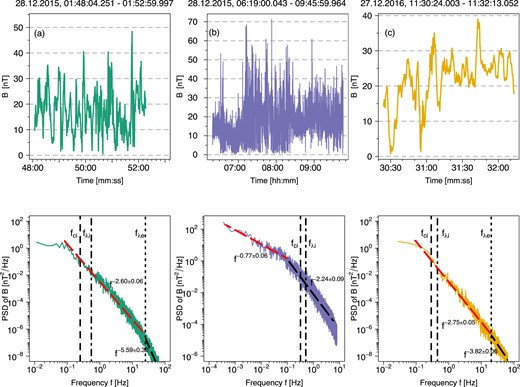
$Time series of the magnetic field strength $B = |\boldsymbol B|$ of the MMS data with the corresponding spectra in the SH (a) near the BS, (b) inside the SH, and (c) near the MP plotted with three different colours. Average ion gyrofrequency (fci), and a characteristic Taylor’s shifted frequencies for ions (fλi) and electrons (fλe) are shown by the dashed, dashed–dotted, and dotted lines, respectively; see table 1 of Macek et al. (2018).$

Figure 1.

Time series of the magnetic field strength |$B = |\boldsymbol B|$| of the MMS data with the corresponding spectra in the SH (a) near the BS, (b) inside the SH, and (c) near the MP plotted with three different colours. Average ion gyrofrequency (f_ci), and a characteristic Taylor’s shifted frequencies for ions (f_λi) and electrons (f_λe) are shown by the dashed, dashed–dotted, and dotted lines, respectively; see table 1 of Macek et al. (2018).

Open in new tab Download slide

The calculated average ion and electron gyrofrequencies are as follows: in case (a) f_ci = 0.25 Hz, and f_ce = 528 Hz; case (b) f_ci = 0.24 Hz and f_ce = 510 Hz; and case (c) f_ci = 0.29 Hz and f_ce = 609 Hz (Macek et al. 2018). In addition, employing the hypothesis according to Taylor (1938), relating time and space scales in this way: |$l = \upsilon _\mathrm{sw} \, \tau$|⁠, where l is a spatial scale and |$\upsilon _\mathrm{sw}$| is the mean velocity of the solar wind flow in the SH, we estimate characteristic inertial frequencies for ions and electrons: in case (a) f_λi = 0.55 Hz and f_λe = 24.5 Hz; case (b) f_λi = 0.41 Hz and f_λe = 18.1 Hz; and case (c) f_λi = 0.45 Hz and f_λe = 20.1 Hz. We have marked these values on each graph of PSD. In case (a) the obtained spectral exponent is about −2.60 ± 0.06 somewhat steeper, before the f_λe = 24.5 Hz threshold and undoubtedly more steepen than the Kolmogorov (1941) (−5/3) or Kraichnan (1965) (−3/2) slopes.

On the other hand, outside the inertial range of scales large spectral exponents has been reported from the Cluster multispacecraft mission (Sahraoui et al. 2009), the WIND data (Bruno, Trenchi & Telloni 2014), including the proposed explanation of nature of solar wind magnetic fluctuations on kinetic scales based on the missions (e.g. Lion, Alexandrova & Zaslavsky 2016; Roberts et al. 2016). Owing to unprecedented high 7.8 ms time resolution of magnetometer data in the MMS mission available in burst mode, we also see that in case (a) the slope is of −2.60 ± 0.06 (close to −5/2) above f_λe = 24.5 Hz. This is further followed by an even steeper spectrum with the slope of −5.59 ± 0.32 (close to −11/2 or −16/3). Because of a substantially lower survey data resolution of 62.5 ms in case (b) the spectrum with −2.24 ± 0.09 (≈−7/3) is steeper than the Kolmogorov (1941) (−5/3) spectrum only after the visible breakpoint in the slope, which lies at f = 0.12 Hz, i.e. near the ion gyrofrequency f_ci = 0.24 Hz, while more gentle slope of −0.77 ± 0.06 is observed before this breakpoint. Finally, in case (c), similarly as in case (a) using BURST data, the spectral exponent of −2.75 ± 0.05 is again steeper before, and even more with the exponent −3.82 ± 0.06 (close to −7/2) after the observed breakpoint that lies at around the electron Taylor’s (1938) shifted frequency f_λe = 20 Hz, as discussed by Macek et al. (2018). This shows that the observed stochastic nature of fluctuations in the subion scale could be due to the interaction between coherent structures (Perrone et al. 2016, 2017), and a very high slope of −16/3 is possibly related to the dissipation of the kinetic Alfvén waves (e.g. Schekochihin et al.2009).

3 METHODS OF DATA ANALYSIS

As usual, we use the fluctuations of the magnetic fields B = |B|, which describe this turbulent system at each time t > 0. Therefore, with a given time-scale τ_i > 0 ∀_i, one can typically define the increments of this quantity as follows:

$$\begin{eqnarray} b_{i} (t) := B (t+\tau _i) - B (t), \end{eqnarray}$$

(1)

and, assuming an arbitrary τ_i > 0, it can be labelled as b_τ or b for simplicity in the following sections.

We assume that the fluctuations of increment b_τ in a larger time-scale τ are transferred to smaller and smaller scales. Therefore, stochastic fluctuations may be regarded as a stochastic process in scale with the N-point joint (transition) conditional probability density function denoted by P(b₁, τ₁|b₂, τ₂, …, b_N, τ_N). In this case, the conditional probability density function is defined by default as

$$\begin{eqnarray} P(b_i,\tau _i|b_j,\tau _j) = \frac{P(b_i, \tau _i; b_j, \tau _j)}{P(b_j,\tau _j)}, \end{eqnarray}$$

(2)

with the marginal (unconditional) probability density function, P(b_j, τ_j), and the joint probability function, P(b_i, τ_i; b_j, τ_j), of finding the fluctuations b_i at a scale τ_i and b_j at a scale τ_j, for 0 < τ_i < τ_j. In the same way, we may construct the conditional probability densities for any longer sequences of increments b.

The stochastic process is Markovian if the conditional probability function depends only on the initial values b₁ and b₂ at the time-scales τ₁ and τ₂, but not on b₃ at the next larger scale τ₃, and so on, i.e. for any i = 1, …, N we have

$$\begin{eqnarray} P(b_1,\tau _1|b_2,\tau _2) = P(b_1,\tau _1|b_2,\tau _2 , ... , b_N,\tau _N) \end{eqnarray}$$

(3)

for 0 < τ₁ < τ₂ < |$\cdots$| < τ_N. Basically, the Markov process can be determined by the initial conditional probability function P(b₁, τ₁|b₂, τ₂). Strictly speaking, the future states of the process are conditionally independent of past states. Because of this relation, the conditional probabilities are also called transition probabilities, while the property of equation (3) is known as a memorylessness.

One of the generalizations of equation (3) is called the Chapman–Kolmogorov (CK) condition, which is given by the equation (Risken 1996)

$$\begin{eqnarray} P(b_1,\tau _1|b_2,\tau _2) = \int _{-\infty }^{+\infty } P(b_1,\tau _1|b^{\prime },\tau ^{\prime }) P(b^{\prime },\tau ^{\prime }|b_2,\tau _2) \, \mathrm{ d} b^{\prime } \end{eqnarray}$$

(4)

for τ₁ < τ′ < τ₂. This equation can be interpreted in the following way: the transition probability from b₂ at a time-scale τ₂ to b₁ at a time-scale τ₁ is the same as a product of the transition probability from b₂ at a time-scale τ₂ to b′ at a time-scale τ′, and the transition probability from b′ at a time-scale τ′ to b₁ at a time-scale τ₁, for all possible b′s. Let us emphasize here that such a generalization is a necessary condition for a stochastic process to be the Markov process.

Next, from the CK condition of equation (4), by using a standard series expansion, one can derive a corresponding Kramers–Moyal (KM) backward expansion with an infinite number of terms. Backward expansions are equations of evolution of probability P(b, τ|b′, τ′), where we differentiate with respect to b. This equation has the following differential form (see section 4.2 of Risken 1996):

$$\begin{eqnarray} {-}\frac{\partial }{\partial \tau } P(b,\tau |b^{\prime }, \tau ^{\prime }) = \sum _{k = 1}^{\infty } \left(-\frac{\partial }{\partial b}\right)^{k} D^{(k)}(b,\tau) P(b, \tau |b^{\prime },\tau ^{\prime }), \end{eqnarray}$$

(5)

where it is important to note that the differential symbol acts on both D^(k)(b, τ) and P(b, τ|b′, τ′) coefficients. Since the solutions of the forward and backward KM equations are equivalent, then without loss of generality, we can label it as KM expansion. Formally, D^(k)(b, τ) are called KM coefficients, which in this way are defined as the limit at |$\tau \to \tau^{\prime}$| of kth power of conditional moments (see Risken 1996):

$$\begin{eqnarray} D^{(k)}(b,\tau) &=& \frac{1}{k!} \lim _{\tau \rightarrow \tau ^{\prime }} \frac{1}{\tau - \tau ^{\prime }} M^{(k)} (b, \tau , \tau ^{\prime }), \end{eqnarray}$$

(6)

$$\begin{eqnarray} M^{(k)} (b, \tau , \tau ^{\prime }) = \int _{-\infty }^{+\infty } (b^{\prime } - b)^{k} P(b^{\prime },\tau ^{\prime }|b,\tau) \, \mathrm{ d} b^{\prime }. \end{eqnarray}$$

(7)

Ideally, using the conditional moments M^(k)(b, τ, τ′), the KM coefficients can be evaluated, though they cannot be obtained directly from the analysed data. While these conditional moments can be calculated from the empirical observations, the D^(k)(b, τ) coefficients can only be obtained by extrapolation in the limit |$\tau \to \tau^{\prime}$| according to equations (6) and (7), but these formulae cannot be applied explicitly.

One of the popular extrapolation methods for this problem is a use of piecewise linear regression model with breakpoints. This is a type of regression model, which allows multiple linear models to fit to the analysed data. The crucial objective of this method is an accurate estimation of a number of breakpoints. First, in order to estimate the best breakpoint position, we have evaluated every value within a specified interval and looked at the value of logarithmic transformation of the likelihood function (also known as log-likelihood function) of each adjusted model. Naturally, the highest value of this function provides the optimal breakpoint. Further, to select (and estimate) the best possible number of breakpoints of the segmented relationship, we have used the standard Akaike (1973) information criterion (AIC) and Bayesian information criterion (BIC; Schwarz 1978). None the less, the truly similar results are obtained when the lowest time resolution is taken. Thus, in our case, we have a simple approximation of the KM coefficients, which is given by

$$\begin{eqnarray} D^{(k)}(b,\tau) = \frac{1}{k!} \frac{1}{\Delta t} M^{(k)} (b, \tau , \tau ^{\prime }), \end{eqnarray}$$

(8)

where Δt is a given lowest time resolution of the time series. It is also interesting to note that D^(k)(b, τ) coefficients show the same dependence on b as M^(k)(b, τ, τ′). This simplification substantially decreases the time required to obtain the results numerically.

Now, in order to find the solution of equation (5), it is necessary to determine the number of terms of the right-hand side (RHS) of this equation that needs to be considered. According to Pawula’s theorem, the KM expansion of a positive transition probability P(b, τ|b′, τ′) may end after the first or second term (e.g. Risken 1996, section 4.3). If it does not end after the second term, then the expansion must contain an infinite number of terms. On the other hand, if the second term is the last one, namely D^(k)(b, τ) = 0 for k ≥ 3, then the KM expansion of equation (5) leads to the following particular formula:

$$\begin{eqnarray} {-}\frac{\partial }{\partial \tau } P(b,\tau |b^{\prime },\tau ^{\prime }) &=& \Bigg [-\frac{\partial }{\partial b} D^{(1)}(b,\tau) + \frac{\partial ^{2}}{\partial b^{2}} D^{(2)}(b,\tau)\Bigg ] \\ && \times P(b,\tau |b^{\prime },\tau ^{\prime }), \end{eqnarray}$$

(9)

with the well-known FP operator |$\mathcal {L}_\mathrm{FP}(b, \tau)$| in the squared parenthesis (e.g. Risken 1996, equations 5.1 and 5.2) governing the evolution of the probability density function P(b, τ|b′, τ′) and is called the FP equation (also known as a forward Kolmogorov equation). It has been primarily used for the Brownian motion of particles, but now equation (9) defines a generalized Ornstein–Uhlenbeck process. Strictly speaking, this is a linear second-order partial differential equation of a parabolic type. By solving the FP equation, it is possible to find distribution functions from which any averages (expected values) of macroscopic variables can be determined by integration. If the relevant time-dependent solution is provided, this equation can be used to not only describe stationary features, but also the dynamics of systems.

The first term, D⁽¹⁾(b, τ), and the second term, D⁽²⁾(b, τ) > 0, determining the FP equation (9) are responsible for the drift and diffusion processes, respectively. The former process accounts for the deterministic evolution of the stochastic process (as a function of b and τ). The latter process modulates the amplitude of the δ-correlated Gaussian noise Γ(τ) (which is known as the Langevin force – the fluctuating force F_f(τ) per unit mass m), that fulfils the normalization conditions: 〈Γ(τ)Γ(τ′)〉 = 2δ(τ − τ′), where δ is a Dirac delta function and 〈Γ(τ)〉 = 0 (see Risken 1996). Thus, in the equivalent approach another complementary equation arises:

$$\begin{eqnarray} {-}\frac{\partial b}{\partial \tau } = D^{(1)}(b,\tau) + \sqrt{D^{(2)}(b,\tau)} \, \Gamma (\tau), \end{eqnarray}$$

(10)

which is formally called the Langevin equation. Here we have used the Itô (1944) definition that is missing a spurious drift (e.g. Risken 1996, section 3.3.3), hence the drift coefficient D⁽¹⁾ occurs directly, unlike in the Stratonovich (1968) definition. Admittedly, the Itô (1944) definition is more difficult to interpret and analyse, because of the new rules for integration and differentiation that must be used. Although, owing to a powerful apparatus, which is the Itô Lemma, it allows us to deal with stochastic processes analytically. Anyway, here again, all higher KM coefficients D^(k) for k ≥ 3 are equal to zero. Note that the negative signs on the left-hand side (LHS) of equations (9) and (10) show that the corresponding transitions proceed backward to smaller and smaller scales.

Next, because the differentiating in the FP operator in equation (9) should act on both the KM coefficients and the conditional probability density P(b, τ|b′, τ′) by performing relatively simple transformations, it can be rewritten in the following expanded form (equation 45.3a of Risken 1996):

$$\begin{eqnarray} &&{-}\frac{\partial }{\partial \tau } P(b,\tau |b^{\prime }, \tau ^{\prime }) = D^{(2)}(b,\tau |b^{\prime }, \tau ^{\prime }) \frac{\partial ^2}{\partial b^2} P(b,\tau |b^{\prime }, \tau ^{\prime }) \\ &&\quad+ \Bigg [2 \frac{\partial }{\partial b} D^{(2)}(b,\tau |b^{\prime }, \tau ^{\prime }) - D^{(1)}(b,\tau |b^{\prime }, \tau ^{\prime })\Bigg ] \frac{\partial }{\partial b} P(b,\tau |b^{\prime }, \tau ^{\prime }) \\ &&\quad+ \Bigg [\frac{\partial ^2}{\partial b^2} D^{(2)}(b,\tau |b^{\prime }, \tau ^{\prime }) - \frac{\partial }{\partial b} D^{(1)}(b,\tau)\Bigg ] P(b,\tau |b^{\prime }, \tau ^{\prime }). \end{eqnarray}$$

(11)

Formally, equation (11) resulting from the FP equation (9) is the second-order parabolic partial differential equation.

It is also worth mentioning that this equation is the generalization of the case of thermal conductivity diffusion equation, which can be solved with the initial and boundary conditions P(b, τ = 0|b′, τ′ = 0) = p(b, b′) and P(b = 0, τ|b′ = 0, τ′) = 0, respectively, using the method of separation of variables. The solution of non-stationary FP equation (11) can well be approximated numerically, i.e. by the difference method. The master curve for the probability density function P(b, τ) of equation (11) can readily be evaluated by the stationary solution p_s(b, τ) of equation (9), which is given by

$$\begin{eqnarray} \frac{\partial }{\partial b} \Big [ D^{(2)}(b,\tau) p_\mathrm{ s}(b, \tau) \Big ] = D^{(1)}(b,\tau) p_\mathrm{ s}(b, \tau) \end{eqnarray}$$

(12)

that results from comparing the LHS of equation (9) with zero.

4 RESULTS

In order to inspect processes responsible for stochastic fluctuations in space plasma, we have applied the methods described in Section 3 to small scale in cases (a) and (c) and medium scale in case (b) fluctuations of the magnetic field B = |B| in the Earth’s SH. In general, the approach presented in this paper could be applied under a few important conditions that should be tested as preliminary procedures (see Rinn et al. 2016). The first condition is that time series data must be stationary. If they were non-stationary, then the conditional moments given by equation (7) are not essentially meaningful. The second condition is that the process should be Markovian, i.e. the present state should only depend on the preceding state. The third condition is that the Pawula’s theorem must hold, as discussed in Section 3.

Having this in mind, we have started with the brief analysis and description of the relevant time series and the corresponding graphs of power spectral densities. Next, we have checked stationarity of all analysed time series (see e.g. Macek 1998). To show that a Markov processes approach is suitable in our situation, we have moved forward to the verification of the necessary CK condition, through estimation of the KM coefficients, and then have checked the validity of the Pawula’s theorem. This lets us to apply the reduced formula of the FP equation (9), which describes evolution of the probability density function P(b, τ).

Following our initial discussion, we must now verify whether the data time series under study is stationary. Generally, if a time series exhibits no trend, has a constant variance over time, and a consistent autocorrelation function over time, then it is classified as stationary. Such time series are also much easier to model. There are a variety of ways to evaluate this feature of any time series. One of such method is the augmented Dickey & Fuller (1979) test. This test uses the following null and alternative hypotheses: H₀: the time series is non-stationary, versus H₁: the time series is stationary. When the p-value is less than 0.05, then the null hypothesis can be rejected and it can be concluded that the time series is stationary. In fact, after performing such a statistical test, we have determined that in cases (a) and (b), the respective p-values are <0.01, indicating that the null hypothesis can be rejected. Thus, these magnetic field strength B = |B| time series are stationary. However, in case (c), where a much smaller data sample is available, the p-value is equal to 0.154, hence we have failed to reject the null hypothesis. The result suggests that the time series is non-stationary and has some time-dependent structure with varying variance over time.

Once again, there are various methods of eliminating trends and seasonality, which define non-stationary time series. Trends can cause the mean to fluctuate over time, while seasonality can lead to changes in the variance over time. The most straightforward approach to address this issue is the differencing technique, a common and frequently used data transformation that is applied for making time series data stationary. Differencing is achieved by subtracting the previous observation from the current one. Following notation in equation (1), this can simply be written as b(t) = B(t) − B(t − 1). To reverse this process, the prior time-step’s observation must be added to the difference value. The practice of computing the difference between successive observations is referred to as a lag-1 difference. The number of times that differencing is carried out is referred to as the order of differentiation. Fortunately, in our case (c), applying the lag-1 (order 1) difference operation has been sufficient to get rid of non-stationarity. The augmented Dickey & Fuller (1979) test has yielded a p-value of less than 0.01, thus the null hypothesis could be rejected, indicating that the analysed B = |B| time series is stationary.

We have used one of the exploratory data analysis approaches called unsupervised binning method (compare with normalized histogram method) to make bins (histogram’s boxes) and to obtain the empirical conditional probability density functions P(b₁, τ₁|b₂, τ₂) for 0 < τ₁ < τ₂ directly from the analysed data. First, we have estimated the empirical joint PDF P(b₁, τ₁; b₂, τ₂) by counting the number of different pairs (b₁, b₂) on a two-dimensional grid of equal width data bins (small intervals). This bins integer should be neither too large, such that each bin no longer contains a significant quantity of points, nor too small, such that any dependency of the drift and diffusion coefficients on the state variable cannot be detected. Next, we have performed the normalization such that the integral over all bins is equal to 1 (note that the sum will not be equal to 1 unless bins of unity width are chosen). Similarly, the empirical one-dimensional PDF P(b₂, τ₂) can be estimated with the use of a one-dimensional grid of bins (and carrying out the normalization), and the empirical conditional PDFs are obtained using equation (2) directly (in a numerical sense).

In such a way, we have found the empirical conditional probability density functions from the analysed data, which are shown by red continuous contours in Fig. 2. They are compared here with the theoretical conditional PDFs that are solutions of the CK condition of equation (4) displayed by blue dashed contours, which are two-dimensional representation of three-dimensional data. Such a comparison is seen in Fig. 2 for the magnetic field increments b, at the various scales: in cases (a) and (c) τ₁ = 0.02 s, τ′ = τ₁ + Δt_B = 0.0278 s, τ₂ = τ₁ + 2Δt_B = 0.0356 s, where Δt_B = 0.0078 s, and in case (b) τ₁ = 0.2 s, τ′ = τ₁ + Δt_B = 0.2625 s, τ₂ = τ₁ + 2Δt_B = 0.325 s, where Δt_B = 0.0625 s. The depicted subsequent isolines correspond to the following decreasing levels of the conditional PDFs, from the middle of the plots, for following magnetic field increments b: case (a) 2, 1.1, 0.5, 0.3, 0.05, 0.01; case (b) 5, 1, 0.7, 0.45, 0.3, 0.22, 0.15, 0.1, 0.05; and case (c) 7, 3.3, 1.3, 0.3, 0.08, 0.06. This is rather evident that the contour lines corresponding to these two empirical and theoretical probability distributions are nearly matching for all three cases. Thus, it appears that the CK condition of equation (4) is sufficiently well satisfied.

Figure 2.

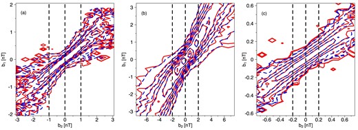
Comparison of observed contours (red solid curves) of conditional probabilities at various time-scales τ, with reconstructed contours (blue dashed curves) according to the Chapman–Kolmogorov (CK) condition, recovered by the use of MMS magnetic field total magnitude B = |B| in the SH: (a) just behind the BS, (b) inside the SH, and (c) near the MP, corresponding to the spectra in Fig. 1.

Open in new tab Download slide

Next, in the corresponding Fig. 3, we have verified again the CK condition of equation (4). Intuitively speaking (and somehow informally), what we see in Fig. 2 is just a view ‘from the top’ of the three-dimensional shape, while in Fig. 3 the orthogonal cuts are depicted. Again, we have compared these cuts through the conditional probability density functions for particular chosen values of parameter b₂, which can be seen at the top of each plot. As is evident, the cuts through the empirical probability density functions coincide rather well with the cuts through the theoretical probability density functions, providing good fits in all of the analysed cases. Admittedly, only in case (b) for b₂ = 0 [nT] the cuts points deviate from the lines in tails, but it seems to be caused by the data outliers, which can eventually be further eliminated. It is necessary to mention that after such a comparison for different values of (τ₁, τ′, τ₂), we have found that the CK condition of equation (4) is satisfied for b up to a scale of approximately 100Δt_B = 0.78 s in case (a), to about 150Δt_B = 9.375 s in case (b), and around 40Δt_B = 0.312 s in case (c), thus indicating that the stochastic fluctuations have Markov properties.

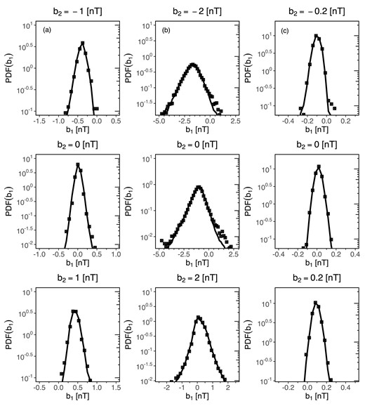
Comparison of cuts through P(b1, τ1|b2, τ2) for the fixed value of the strength of the magnetic field total magnitude B = |B| in the SH: (a) just behind the BS, (b) inside the SH, and (c) near the MP, with increments b2 with τ1 = 0.02 s, τ′ = 0.0278 s, and τ2 = 0.0356 s in cases (a) and (c), and with τ1 = 0.2 s, τ′ = 0.2625 s, and τ2 = 0.325 s in case (b).

Figure 3.

Comparison of cuts through P(b₁, τ₁|b₂, τ₂) for the fixed value of the strength of the magnetic field total magnitude B = |B| in the SH: (a) just behind the BS, (b) inside the SH, and (c) near the MP, with increments b₂ with τ₁ = 0.02 s, τ′ = 0.0278 s, and τ₂ = 0.0356 s in cases (a) and (c), and with τ₁ = 0.2 s, τ′ = 0.2625 s, and τ₂ = 0.325 s in case (b).

Open in new tab Download slide

To verify Pawula’s theorem, which states that if the fourth-order coefficient is equal to zero, then D^(k)(b, τ) = 0, k ≥ 3, it is necessary to estimate the D⁽¹⁾(b, τ), D⁽²⁾(b, τ), and D⁽⁴⁾(b, τ) coefficients using our experimental data. The standard procedure for calculating these values is to use an extrapolation method such as a piecewise linear regression to estimate the respective limits in equation (6). However, as already mentioned in Section 3, the similar results are obtained by simplifying the problem of finding these coefficients, by using equation (8), which enables us to estimate these values using the adequately scaled M^(k)(b, τ, τ′) coefficients. In our situation, the time resolution Δt_B is equal to 7.8 ms in cases (a) and (c), while in case (b) it is 62.5 ms. Thus, given the conditional probabilities P(b₁, τ₁|b₂, τ₂) for 0 < τ₁ < τ₂, we have calculated these central moments directly from equation (7), using the obtained empirical data by counting the numbers N(b′, b) of occurrences of two fluctuations b′ and b. Given that the errors of N(b′, b) might be simply determined by |$\sqrt{N(b^{\prime },b)}$|⁠, then, in a similar way, it is possible to calculate the errors for the conditional moments M^(k)(b, τ, τ′). Consequently, scaling these values according to equation (8), we have obtained the empirical KM coefficients. By examination of the M^(k)(b, τ, τ′) and D^(k)(b, τ) coefficients, we can observe that they both exhibit the same dependence on b.

The results of this analysis are shown in Fig. 4, where on the upper part we have depicted the first-order coefficient depending on b, while at the bottom we have shown the second- and fourth-order coefficients depending on b, for all three cases (a), (b), and (c). Moreover, for each case, we have provided the calculated confidence intervals (error bars). It is demonstrated that the fit for D⁽¹⁾(b, τ) coefficient is a linear function of b and for D⁽²⁾(b, τ) is a quadratic function of b, for Δt_B = 0.0078 s in cases (a) and (c), and Δt_B = 0.0625 s in case (b). In fact, we have checked that the same fits are reasonable up to even 150Δt_B for all three analysed cases. This means that in this instance, there should be no difficulties with fitting the polynomials for different Δt_B.

Figure 4.

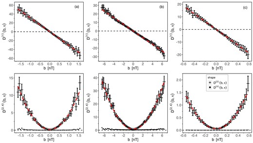
The first and second limited-size Kramers–Moyal (KM) coefficients determined by the magnetic field increments b for a total strength of magnetic field B = |B| in the SH: (a) just behind the BS, (b) inside the SH, and (c) near the MP. The dashed red lines show the best choice fits to the calculated values of D⁽¹⁾(b, τ) and D⁽²⁾(b, τ) with D⁽⁴⁾(b, τ) = 0, according to the Pawula’s theorem.

Open in new tab Download slide

As seen at the bottom part of Fig. 4 of cases (a) and (c), it is evident that the Pawula’s theorem is clearly satisfied. On the other hand, in case (b) it might be not so obvious. For instance, for b ≈ −6.2 nT, we can see that the value of D⁽⁴⁾(b, τ) is somewhat greater than zero. In this case, we can use the somewhat weaker version of this theorem, which states that it is sufficient to check if D⁽⁴⁾(b, τ) ≪ [D⁽²⁾(b, τ)]², for all b (see Risken 1996; Rinn et al. 2016). Thus, in this situation, we have [D⁽²⁾(b, τ)]² ≈ 1225, which is significantly larger than D⁽⁴⁾(b, τ) ≈ 1, for b ≈ −6.2 nT. Therefore, it is reasonable to conclude that the Pawula’s theorem is sufficiently well fulfiled in all of the analysed cases. Hence we can assume that the Markov process is described by the FP equation (9).

In order to find the analytical solution of the FP equation (9), we have proposed certain approximations of the lowest order KM coefficients. As previously discussed (see Fig. 4), it is straightforward that D⁽¹⁾(b, τ) exhibits a linear dependence, whereas D⁽²⁾(b, τ) displays a quadratic dependence on b. Consequently, it is reasonable to assume the following parametrization:

$$\begin{eqnarray} \left\lbrace \begin{aligned} D^{(1)} (b, \tau) & = - a_1 (\tau) b, \\ D^{(2)} (b, \tau) & = a_2 (\tau) + b_2 (\tau) b^2, \end{aligned} \right. \end{eqnarray}$$

(13)

where the relevant parameters a₁ > 0, a₂ > 0, and b₂ > 0 depend on temporal scale τ > 0. Moreover, it appears that all of these parameters exhibit a power-law dependence on temporal scale τ:

$$\begin{eqnarray} \left\lbrace \begin{aligned} a_1(\tau) = A \tau ^{\alpha }, \\ a_2(\tau) = B \tau ^{\beta }, \\ b_2(\tau) = C \tau ^{\gamma }, \end{aligned} \right. \end{eqnarray}$$

(14)

where the values for all of the logarithmized parameters |$A, B, C \in \mathbb {R}$| and the |$\alpha , \beta , \gamma \in \mathbb {R}$| are given in Table 1.

Table 1.

Open in new tab

The fitted parameters for power-law dependence of first- and second-order Kramers–Moyal (KM) coefficients of equations (13) and (14) as functions of scale τ.

Case	log₁₀(A)	α	log₁₀(B)	β	log₁₀(C)	γ
(a)	0.6989 ± 0.0225	−1.1191 ± 0.0089	−0.4946 ± 0.1259	1.1631 ± 0.0498	0.5854 ± 0.0706	−1.7325 ± 0.0279
(b)	0.1837 ± 0.0139	−1.0417 ± 0.0100	−0.4666 ± 0.0160	0.5425 ± 0.0116	0.4183 ± 0.0163	−1.2233 ± 0.0118
(c)	0.7791 ± 0.0079	−1.1055 ± 0.0057	−0.5893 ± 0.0126	1.0002 ± 0.0091	0.5011 ± 0.0274	−1.7646 ± 0.0199

Case	log₁₀(A)	α	log₁₀(B)	β	log₁₀(C)	γ
(a)	0.6989 ± 0.0225	−1.1191 ± 0.0089	−0.4946 ± 0.1259	1.1631 ± 0.0498	0.5854 ± 0.0706	−1.7325 ± 0.0279
(b)	0.1837 ± 0.0139	−1.0417 ± 0.0100	−0.4666 ± 0.0160	0.5425 ± 0.0116	0.4183 ± 0.0163	−1.2233 ± 0.0118
(c)	0.7791 ± 0.0079	−1.1055 ± 0.0057	−0.5893 ± 0.0126	1.0002 ± 0.0091	0.5011 ± 0.0274	−1.7646 ± 0.0199

Table 1.

Open in new tab

The fitted parameters for power-law dependence of first- and second-order Kramers–Moyal (KM) coefficients of equations (13) and (14) as functions of scale τ.

Case	log₁₀(A)	α	log₁₀(B)	β	log₁₀(C)	γ
(a)	0.6989 ± 0.0225	−1.1191 ± 0.0089	−0.4946 ± 0.1259	1.1631 ± 0.0498	0.5854 ± 0.0706	−1.7325 ± 0.0279
(b)	0.1837 ± 0.0139	−1.0417 ± 0.0100	−0.4666 ± 0.0160	0.5425 ± 0.0116	0.4183 ± 0.0163	−1.2233 ± 0.0118
(c)	0.7791 ± 0.0079	−1.1055 ± 0.0057	−0.5893 ± 0.0126	1.0002 ± 0.0091	0.5011 ± 0.0274	−1.7646 ± 0.0199

Case	log₁₀(A)	α	log₁₀(B)	β	log₁₀(C)	γ
(a)	0.6989 ± 0.0225	−1.1191 ± 0.0089	−0.4946 ± 0.1259	1.1631 ± 0.0498	0.5854 ± 0.0706	−1.7325 ± 0.0279
(b)	0.1837 ± 0.0139	−1.0417 ± 0.0100	−0.4666 ± 0.0160	0.5425 ± 0.0116	0.4183 ± 0.0163	−1.2233 ± 0.0118
(c)	0.7791 ± 0.0079	−1.1055 ± 0.0057	−0.5893 ± 0.0126	1.0002 ± 0.0091	0.5011 ± 0.0274	−1.7646 ± 0.0199

It is important to emphasize that the functional dependencies of the coefficients a₁(τ), a₂(τ), and b₂(τ) on τ given by equation (14) are merely parametrizations of the empirical results. In fact, here power laws have been selected, because they have adequately described the observed values with sufficient accuracy. Nevertheless, some alternative theoretical analyses may lead to slightly different functional dependence (see Renner et al. 2001). Admittedly, it turned out that the values of the fitted parameters can slightly be different from those that fit exactly the solution of the FP equation (9). Renner et al. (2001) have also highlighted the asymmetry of the fit D⁽²⁾(b, τ) on b, which is also present in our analysis [especially in case (c), and to a lesser degree in case (a)].

The obtained fits to the MMS observations in the SH are depicted in Fig. 5, for each case (a), (b), and (c), showing the dependence of KM coefficients parameters on scale τ > 0. Since our data contain a multitude of relatively low values and a few exceedingly large values, which would render a linear graph rather unreadable, instead of using a standard linear graph, we have decided to employ logarithmic scales for both the vertical and horizontal axes (so-called log –log plot). Such a procedure is rather straightforward. For example, for the first row of equation (14), taking the logarithm of both sides one obtains log (a₁(τ)) = α log (τ) + log (A), which is a special case of a linear function, with the exponent α corresponding to the slope of the line. The value of log (A) corresponds to the intercept of a log (a₁(τ)) axis, while the log (τ) axis is intercepted at log A/(−α). We have opted for this approach to enhance the clarity of the presentation. Therefore, since we have used both the logarithmic scales the respective power laws appear as straight lines in Fig. 5. Similarly, the graphical representations for all the parameters a₁, b₁, and b₂ of equations (13) and (14), which we have provided, are helpful for identifying correlations and determining respective constants A, B, C and α < 0, β > 0, γ < 0 in Table 1 (cf. Macek et al. 2023).

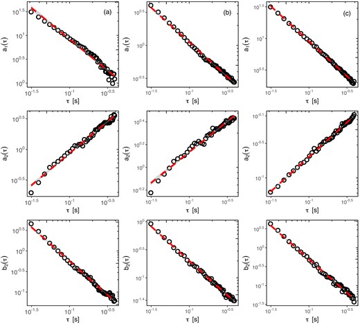
Linear dependence of the parameters a1, a2, b2 (see equation 14) on the double logarithmic scale τ (log–log plot), for the magnetic field overall intensity B = |B| in the SH: (a) just behind the BS, (b) inside the SH, and (c) near the MP. The dashed red lines, with the standard error of the estimate illustrated by grey shade, show the best choice fits to the calculated values.

Figure 5.

Linear dependence of the parameters a₁, a₂, b₂ (see equation 14) on the double logarithmic scale τ (log–log plot), for the magnetic field overall intensity B = |B| in the SH: (a) just behind the BS, (b) inside the SH, and (c) near the MP. The dashed red lines, with the standard error of the estimate illustrated by grey shade, show the best choice fits to the calculated values.

Open in new tab Download slide

After performing a careful analysis of the MMS magnetic field magnitude B data, our findings indicate that the power-law dependence is applicable for the values of: τ ≲ 100Δt_B = 0.78 s in case (a); τ ≲ 150Δt_B = 9.375 s in case (b); τ ≲ 50Δt_B = 0.39 s in case (c), and for some larger scales, say τ ≳ τ_G, the shapes of the probability density functions appear to be closer to Gaussian. However, despite the satisfactory results obtained at these small kinetic scales, a more intricate functional dependence (possibly polynomial fits) is characteristic for much higher scales, in particular, in the inertial domain (Strumik & Macek2008a,b).

As a result of our investigations, we are able to obtain analytical stationary solutions p_s(x) given by equation (12) following from the FP equation (9), which can be expressed by a continuous kappa distribution (also known as Pearson’s type VII distribution), which exhibits a deviation from the normal Gaussian distribution. The probability density function of this distribution is of a given form

$$\begin{eqnarray} p_\mathrm{ s}(b) = \frac{N_0}{\left [1 + \frac{1}{\kappa } \Big (\frac{b}{b_0}\Big)^2\right ]^{\kappa }}, \end{eqnarray}$$

(15)

where, for a₂(τ) ≠ 0, b₀(τ) ≠ 0, we have a shape parameter κ = 1 + a₁(τ)/[2b₂(τ)] and |$b_0^2 = a_2(\tau) / [b_2(\tau) + a_1(\tau)/2]$|⁠, while N₀ = p_s(0) satisfies the normalization |$\int _{- \infty }^{\infty } p_\mathrm{ s}(b) \, \mathrm{ d}b = 1$|⁠. By substituting p_s(b) to this integral we find that

$$\begin{eqnarray} N_0 = \frac{\Gamma (\kappa)}{\Gamma \left(\kappa - \frac{1}{2}\right) b_0 \sqrt{\pi \kappa }}, \end{eqnarray}$$

(16)

where, this time, |$\Gamma (\kappa) = \int _0^{\infty } b^{\kappa - 1} \, \mathrm{e}^{-b} \, \mathrm{ d}b$|⁠, Re(κ) > 0 is a mathematical gamma function (Euler integral of the second kind), as defined for all complex numbers with a positive real part.

It is worth noting that kappa distribution, as represented by equation (15), approaches the normal Gaussian (Maxwellian) distribution for large values of scaling parameter κ. To be precise, as κ → ∞, the following well-known formula can approximately be satisfied:

$$\begin{eqnarray} \lim _{\kappa \rightarrow \infty } p_\mathrm{ s} (b) = N_0 \, \exp \Big ({-}\frac{b^2}{2\sigma ^2}\Big), \end{eqnarray}$$

(17)

with the scaling parameter b₀ related to the standard deviation |$\sigma = b_0/\sqrt{2}$|⁠. This time the parameter N₀ = p_s(0) satisfies the elementary normalization |$N_0 = \frac{1}{\sigma \sqrt{2 \pi }}$|⁠.

The numerical results of fitting the empirical MMS data to the given distributions and determining the relevant parameters of equation (15) are as follows: κ = 1.5179, b₀ = 1.9745, and N₀ = 0.68438 for B in case (a); κ = 1.3758, b₀ = 2.6955, and N₀ = 0.34375 in case (b); and κ = 3.5215, b₀ = 1.7313, and N₀ = 1.1866 in case (c). These values of κ would correspond to the non-extensivity parameter of the generalized (Tsallis) entropy q = 1 − 1/κ (e.g. Burlaga & Viñas 2005). In our case this is given by |$q = \frac{a_1(\tau)}{a_1(\tau) + 2 b_2(\tau)}$| and is equal to 0.341 in case (a), 0.273 in case (b), and 0.716 in case (c). The extracted values of the κ and q parameters provide robust measures of the departure of the system from equilibrium. We see that these values are similar to q ∼ 0.5 for κ ∼ 2 reported for the Parker Solar Probe (PSP) data by Benella et al. (2022).

Now, by using the system of equation (13) with equation (9), we have arrived at the following formula (Macek et al. 2023):

$$\begin{eqnarray} &&\big (a_2(\tau) + b_2(\tau) b^2 \big) \frac{\partial ^2 P(b, \tau)}{\partial b^2} + \big (a_1(\tau) + 4 b_2(\tau) \big) b \frac{\partial P(b, \tau)}{\partial b} \\ &&\qquad + \frac{\partial P(b, \tau)}{\partial \tau } + \big (a_1(\tau) + 2 b_2(\tau) \big) P(b, \tau) = 0. \end{eqnarray}$$

(18)

This implies that the FP equations (11) and (18) are expressed in terms of a second-order parabolic partial differential equation. Thus, through the implementation of the numerical Euler integration scheme, which has been verified for stationary solution |$\frac{\partial P(b, \tau)}{\partial \tau } = 0$|⁠, we are able to successfully solve the non-stationary FP equation numerically. Our results are in line with those obtained by Rinn et al. (2016) using the statistical modelling package in programming language r.

Fig. 6 shows the findings resulting from our analysis based on the MMS data. Here we compare the solutions of the FP equation (9) with the empirical probability density functions of P(b, τ): (a) near the BS; (b) inside the SH; and (c) near the MP for various scales τ (not greater than τ_G). The displayed plotted curves, in each case, are as follows: the stationary solution (denoted by open circles); the non-stationary solutions (marked with dashed lines); and the empirical PDFs (indicated with various coloured continuous lines).

Figure 6.

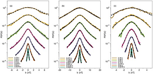
The empirical probability density functions (various continuous coloured lines) for a total strength of magnetic field B = |B|, which correspond to spectra in Fig. 1, compared with the non-stationary (dashed lines) and the stationary (open circles) solutions of the FP equation, for various time-scales (shifted from bottom to top) τ = 0.0078, 0.04, 0.078, 0.12, 0.2, 0.39, and 0.78 s in cases (a) and (c), and τ = 0.0625, 0.3125, 0.625, 0.9375, 1.5625, 3.125, and 9.375 s in case (b).

Open in new tab Download slide

Further, in cases (a) and (c) the corresponding time scales are τ = 0.0078, 0.04, 0.078, 0.12, 0.2, 0.39, and 0.78 s, whereas in case (b) these scales are τ = 0.0625, 0.3125, 0.625, 0.9375, 1.5625, 3.125, and 9.375 s. The corresponding curves are shifted in the vertical direction from bottom to top for even better clarity of presentation. It is also worth noting that we have used the semi-logarithmic scale τ, what is useful when dealing with data that covers a broad range of values. On this scale, the vertical scale is logarithmic (base 10) axis, which means that the separation between the ticks on the graph is proportional to the logarithm of PDF, while the horizontal b-axis is a standard linear scale, and the ticks are evenly spaced.

What is important to note from this picture are the peaked leptokurtic shapes of PDFs and corresponding stationary solutions. Namely, in case (a) the peak (with large kurtosis) is present for scales up to ∼0.5 s; in case (b) up to about ∼3 s; and in case (c) up to ∼0.25 s. For these levels selected for each case the PDF becomes closer to Gaussian (i.e. approximately parabolic shape on the graph with the semi-logarithmic scales), as expected for large values of κ. In case (c) we can see more jumps in fluctuations, i.e. the curves are not so smooth. Fluctuations are quite evident in both the empirical curves and the theoretical solutions, so it seems that some numerical noise is present in the tails of the PDFs. Admittedly, reducing noise is a tricky issue, although the easiest way is to artificially smooth using the simple moving average. Therefore, we have tried this procedure for n = 1, 2, 3 steps and it has appeared that the n = 3 choice is sufficient.

Fig. 7 depicts finally the probability density functions of fluctuations of the strength of the magnetic field b_τ rescaled by the standard deviations σ(b_τ) in the following way:

$$\begin{eqnarray} b_{\tau } \longrightarrow \frac{b_{\tau }}{\sigma (b_{\tau })}, \end{eqnarray}$$

(19)

$$\begin{eqnarray} \text{PDF}(b_{\tau }) &\longrightarrow \sigma (b_{\tau }) \, \text{PDF}(b_{\tau }). \end{eqnarray}$$

(20)

In this way, we can define a master curve for the shape of the PDFs. Again, we have used the logarithmic scale on the vertical axis. We also see that the rescaled curves are consistent with the stationary solutions of equation (15), as marked with open circles in Fig. 6. It should be noted that all the curves in Fig. 7 are very close to each other for small scales. However, for larger τ = 50 or 100Δt_B these shapes deviate from the master curve and naturally tend to the well-known Gaussian shape. We see that the shape of the PDFs obtained from the MMS data exhibits a global scale invariance in the SH up to scales of ∼2 s. A similar collapse has also been reported with the PSP data at subproton scales (Benella et al. 2022). Fig. 7 shows that fluctuations in the SH are described by a stochastic process. Admittedly, the mechanism of generation of these magnetic fluctuation at small kinetic scale is not known, but the results suggest some universal characteristics of the processes. An alternative point of view has recently been proposed by Carbone et al. (2022).

Figure 7.

A collapse of probability density functions of b_τ (compare Fig. 6), which are scaled by the corresponding standard deviations (see equations 19 and 20), for the small time-scales τ stopping at approximately: τ ∼ 0.4 s in case (a); τ ∼ 2.0 s in case (b); and τ ∼ 0.25 s in case (c).

Open in new tab Download slide

5 CONCLUSIONS

Following our studies in the space plasmas at large inertial scales (Strumik & Macek 2008a,b), we have examined time series of the strength of magnetic fields in different regions of the Earth’s SH, where the spectrum steepens at subproton scales (Macek et al. 2018). With the highest resolution available on the MMS, the data samples just after the BS and near the MP are stationary and for somewhat lower resolution deep inside the SH the deviations from stationarity are small and could well be eliminated. Basically, in all these cases the stochastic fluctuations exhibit Markovian features. We have verified that the necessary CK condition is well satisfied, and the probability density functions are consistent with the solutions of this condition.

In addition, the Pawula’s theorem is also well satisfied resulting in the FP equation reduced to drift and diffusion terms. Hence, this corresponds to the generalization of Ornstein–Uhlenbeck process. Further, the lowest KM coefficients have linear and quadratic dependence as functions of the magnetic field increments. In this way, the power-law distributions are well recovered throughout the entire SH. For some moderate scales we have the kappa distributions described by various peaked shapes with heavy tails. In particular, for large values of the kappa parameter these distributions are reduced to the normal Gaussian distribution.

Similarly as for the PSP data, the probability density functions of the magnetic fields measured onboard the MMS rescaled by the respective standard deviations exhibit a universal global scale invariance on kinetic scales, which is consistent with the stationary solution of the FP equation. We hope that all these results, especially those reported at small scales, are important for a better understanding of the physical mechanism governing turbulent systems in space and laboratory.

ACKNOWLEDGEMENTS

We thank Marek Strumik for discussion on the theory of Markov processes. We are grateful for the efforts of the entire MMS mission, including development, science operations, and the Science Data Center at the University of Colorado. We benefited from the efforts of T. E. Moore as Project Scientist, C. T. Russell, and the magnetometer team. We acknowledge B. L. Giles, Project Scientist, for information about the magnetic field instrument, and also D. G. Sibeck and M. V. D. Silveira for discussions during previous visits by WMM to the NASA Goddard Space Flight Center.

This work has been supported by the National Science Centre, Poland (NCN) through grant no. 2021/41/B/ST10/00823.

DATA AVAILABILITY

The data supporting the results in this paper are available through the MMS Science Data Center at the Laboratory for Atmospheric and Space Physics (LASP), University of Colorado, Boulder: https://lasp.colorado.edu/mms/sdc/public/. The magnetic field data from the magnetometer are available online from http://cdaweb.gsfc.nasa.gov. The data have been processed using the statistical programming language r.

References

Akaike

1973

, in

Petrov

B. N.

Csaki

, eds,

Proceedings of the 2nd International Symposium on Information Theory

Akademiai Kiado

Budapest

, p.

267

Month:	Total Views:
September 2023	41
October 2023	56
November 2023	139
December 2023	27
January 2024	65
February 2024	31
March 2024	37
April 2024	30
May 2024	33
June 2024	31
July 2024	29
August 2024	13
September 2024	23
October 2024	33
November 2024	14
December 2024	20
January 2025	11
February 2025	11
March 2025	13
April 2025	16
May 2025	3

Article Contents

Statistical analysis of stochastic magnetic fluctuations in space plasma based on the MMS mission

ABSTRACT

1 INTRODUCTION

2 DATA

3 METHODS OF DATA ANALYSIS

4 RESULTS

5 CONCLUSIONS

ACKNOWLEDGEMENTS

DATA AVAILABILITY

References

Citations

Views

Altmetric

Email alerts

Astrophysics Data System

Citing articles via

Latest

Most Read

Most Cited

This Feature Is Available To Subscribers Only