


ABSTRACT
The aim of this work is to study the anisotropic weak lensing signal associated with the mass distribution of massive clusters of galaxies using the cosmic microwave background (CMB) data. For this purpose, we stack patches of the Planck Collaboration (2018) CMB lensing convergence map centred on SDSS DR8 redMaPPer clusters within the redshift range [0.4, 0.5]. We obtain mean radial profiles of the convergence parameter κ finding strong signals at scales as large as 40 Mpch−1. By orienting the clusters along their major axis defined through the galaxy member distribution, we find a significant difference between the parallel and perpendicular-oriented convergence profiles. The amplitude of the profile along the parallel direction is about 50 per cent larger than that along the perpendicular direction, indicating that the clusters are well aligned with the surrounding mass distribution. From a model with an anisotropic surface mass density, we obtain a suitable agreement for both mass and ellipticities of clusters compared to results derived from weak lensing shear estimates, finding strong evidence of the correlation between the galaxy cluster member distribution and the large-scale mass distribution.
1 INTRODUCTION
Cluster masses have been widely used to restrict cosmological parameters (Burenin & Vikhlinin 2012; Cusworth et al. 2014). In fact, the abundance of clusters above a given mass threshold provides a powerful constrain in ΩM and σ8 parameters (e.g. Abdullah et al. 2022; Lesci et al. 2022).
Among the different methods to infer cluster masses, weak lensing techniques give reliable estimations since they are less affected by the dynamical state of the clusters (McClintock et al. 2019; Murray et al. 2022). Besides, unlike other techniques such as those based on X-ray measurements, the weak lensing method has the advantage of being unaffected by astrophysical sources in the clusters that could bias estimates.
In numerical simulations, clusters show triaxial shapes (Herbonnet et al. 2022), elongated mainly due to the anisotropic large-scale structure and the related accretion process. For this reason, to accurately reproduce the measured density distribution, a two halo anisotropic term must be included (Gonzalez et al. 2022). On the observational side, however, cluster shapes can be only obtained in projection through different tracers such as the member galaxy distribution, intracluster light, X-rays hot emitting gas, and weak lensing. Previous weak lensing studies based on shear measurements (Clampitt & Jain 2016; van Uitert et al. 2017; Shin et al. 2018; Gonzalez et al. 2021) have added evidence for cluster haloes with an average ellipticity parameter |$\epsilon = \frac{1-q}{1+q} \sim 0.2$|, where q is the semi-axes relation, q ≤ 1. These studies are mainly focused on the analysis of the shape of the cluster halo host, neglecting the contribution of the extended mass distribution. On the other hand, related with the surrounding mass distribution in galaxy clusters, Geller et al. (2013), Fong et al. (2018), and Shin et al. (2021) have analysed the expected lensing signal at intermediate scales without fitting the expected elongation at these regions. In this sense, the cosmic microwave background (CMB) lensing signal can be useful to explore the surrounding mass distribution given its large angular extension.
In this paper, we study the convergence map derived from the Planck 2018 lensing data (Planck Collaboration 2020a) around massive clusters of the SDSS DR8 redMaPPer catalogue (Rykoff et al. 2016). This catalogue provides an homogeneously selected sample of massive clusters M ≳ 1014M⊙, suitable for our analysis. We explore the anisotropies imprinted in the CMB convergence map due to the elongation of the extended surface mass distribution, by orientating the maps taking into account the positions of the cluster galaxy members. In this way, we study the anisotropies of the mass distribution beyond the virial region, in close relation to the large-scale structure. Geach & Peacock (2017) also study the redMaPPer clusters catalogue using the Planck 2018 lensing data. Unlike the present work, the authors analyse smaller CMB reprojected regions of 1° around the position of each cluster onto a tangential sky projection with a high-resolution scale of 256 pixels per degree. For this reason, it is observed only a significant signal in the cluster centre neighbourhood, up to 10 arcmin or around ∼3 Mpch−1. Here, we focus on a large-scale study with the aim of analysing extended anisotropic mass distribution around clusters.
The paper is organized as follows: in Section 2, we detail the data of the CMB lensing map and the cluster catalogue. In Section 3, we analyse the mean convergence profiles. In Section 4, we describe an anisotropic model that allows us to trace the extended mass distribution and also explore mean masses and ellipticities of the systems. Finally, in Section 5, we present a brief summary and discussion of our studies.
2 DATA
2.1 CMB convergence map
In the thin lens approximation (see for instance Meneghetti 2022, and references therein), the Laplacian of the effective lens potential in the lens plane takes the form:
where Φ is the tri-dimensional Newtonian potential defined at a given position in the lens plane, |$\vec{\theta }$|, and at redshift z. DL, DS, and DLS are the angular diameter distances from the observer to the lens, from the observer to the source, and from the lens to the source, respectively, involved in the lens system. The adimensional convergence parameter κ is proportional to the effective lens potential by:
which is related to the surface mass density through
where ΣCR is the critical surface density:
The observed CMB photons arises from the last-scattering surface, and along their path, each wavelength are affected by both the expansion of the Universe as well as by the mass inhomogeneities (Blanchard & Schneider 1987). Once the structure in the Universe has grown to form, among other systems, clusters of galaxies, each photon crosses several lenses generated by these systems, resulting in a correlation between certain multipoles l that would otherwise have been independent of each other and therefore secondary non-Gaussian anisotropies (Zaldarriaga & Seljak 1998) are introduced. Given this, for the CMB photons, the effective lens potential represents an integrated measurement of the mass distribution from the observer to the last scattering surface:
where χ* is the comoving distance up to the last scattering surface and |$\Psi (\chi ,\mathbf {\hat{n}})$| is the Weyl potential, in comoving coordinates.
Following the formalism proposed in Planck Collaboration (2016), which involves equations (2) and (4), the Planck Collaboration provides the kLM coefficients:
which allows to reconstruct the CMB convergence map.
In our analysis, we use the data products released in 2018 by the Planck Collaboration (2020a), hereafter PR3. We reconstruct the map from the spherical harmonics coefficients kLM provided by the PR3 release1, using all the L′s available (LMax = 4096) with a FWHM Gaussian kernel of 1°, which is consistent with the range of L′s used in CMB power-spectrum analyses (Mirmelstein, Carron & Lewis 2019; Planck Collaboration 2020a). These coefficients are derived from SMICA DX12 CMB maps (from temperature only after mean field subtraction, TT).2 For an appropriate analysis, we also use the confidence mask provided by PR3 release that eliminates the most relevant astrophysical effects of galactic and extragalactic objects imprinted in the temperature CMB maps.
For the reconstruction and visualization, we use the healpix3 software (Górski et al. 2005). It allows us to transform the kLM coefficients to a map with a resolution given by Nside = 2048. The pixel area has a constant value of AP = 1.062 × 10⁴ arcsec2.
In order to further check the consistency of our methods and results, we also use the PR3 minimum variance (MV) kLM and the TT and MV kLM reconstructed coefficients (Carron, Mirmelstein & Lewis 2022) corresponding to the NPIPE processing pipeline (Planck Collaboration 2020b) (hereafter PR4).
In Fig. 1, we present the CMB lensing map reconstruction, from PR3 TT kLM coefficients, with a FWHM Gaussian kernel smoothing of 5° together with the distribution of redMaPPer clusters, which will be presented in the next section.
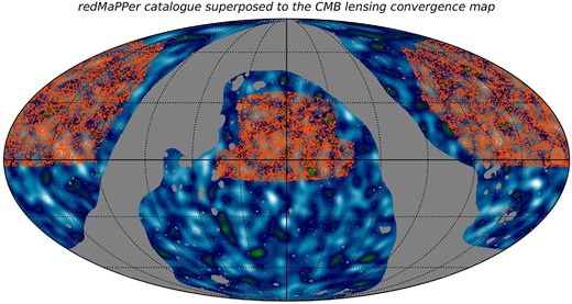
redMaPPer cluster positions (red points) superposed to the CMB lensing convergence map in equatorial mollview projection. The lensing map has a FWHM Gaussian smoothing of 5° for a better visualization. The mask provided by PR3 associated to galactic and extragalactic sources is shown in grey.
2.2 Cluster samples
We analyse samples derived from the redMaPPer cluster catalogue Rykoff et al. (2016) that are identified through a red-sequence algorithm (Rykoff et al. 2014) applied to galaxy overdensities inferred from a percolation procedure on the Sloan Digital Sky Survey Data Release 8 (York et al. 2000; Aihara et al. 2011). This catalogue comprises 26 111 galaxy systems with an angular coverage of 10 401 square degrees in the redshift range [0.08, 0.6]. The catalogue provides a richness parameter, λ, which is a suitable proxy of cluster mass (e.g. Simet et al. 2017; Pereira et al. 2018). This parameter, ranging between 20 and 300, is defined as the sum of the galaxy cluster membership probabilities over all galaxies within a scale-radius Rλ:
where θL and θR are weights associated to a fixed threshold in luminosity and radius.
In our analysis, we restrict both redshift z and richness parameter λ ranges to define several samples that are presented in Table 1 together with their main characteristics. The mean mass 〈M〉 is calculated according to the relation given by Simet et al. (2017). Also, we consider clusters within the CMB lensing mask region.
Main characteristics of cluster samples. The mean mass 〈M〉 is calculated following the procedure in Simet et al. (2017).
| Sample | Number of clusters | Redshift z range | 〈z〉 | Richness parameter λ range | 〈λ〉 | 〈M〉 (M⊙) |
|---|---|---|---|---|---|---|
| S1 | 3000 | [0.4, 0.45] | 0.427 | [31.7, 100] | 44.914 | 1014.304 |
| S2 | 2774 | [0.45, 0.5] | 0.475 | [31.7, 100] | 47.818 | 1014.374 |
| S3 | 1574 | [0.4, 0.45] | 0.420 | [21, 31.7] | 27.797 | 1014.027 |
With the purpose of defining homogeneous samples not strongly affected by redshift nor richness bias, we first consider the redshift range 0.4 ≤ z < 0.45 and select two richness ranges: 21 ≤ λ ≤ 31.7 for sample S3 and 31.7 < λ ≤ 100 for sample S1. We adopt the threshold λ = 31.7 that corresponds to the 3000 richer clusters of sample S1. Additionally, we impose an upper limit λ ≤ 100 to avoid spuriously high λ values probably associated to biases in the percolation procedure. Then, we consider the same richness interval (31.7 < λ ≤ 100) with a different redshift range: 0.45 ≤ z ≤ 0.5 for sample S2. We avoid the use of clusters with redshift lower than 0.4, which are not well suitable for this analysis due to their lower lensing signal.
In the upper-left panel of Fig. 2, we show the richness-redshift (λ − z) distribution for the catalogue that is complete in richness up to z ∼ 0.4. In the upper-right panel, we show the sample S1. As it can be seen in this figure, this restricted area provides a quasi-homogeneous distribution of richness parameter λ across the redshift interval. We present sample S2 in the lower-left panel, where we can see that this region also provides a nearly homogeneous distribution across redshift, similarly to sample S1. In the lower-right panel, we display sample S3. This sample, contrary to S1 and S2, is not complete in richness.
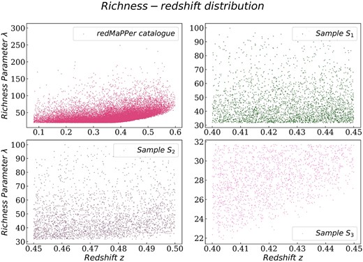
Richness-redshift (λ − z) distribution. Upper-left panel: redMaPPer catalogue. It can be seen an excess of high values of λ at higher z. Upper-right panel: Sample S1. Richness is distributed nearly homogeneous across the redshift interval. Lower-left panel: Sample S2. Here, richness is also distributed nearly homogeneous across the redshift interval. Lower-right panel: Sample S3. The observed excess of high values of λ at higher z can induce a bias in the convergence analysis.
Some main features can be deduced from Table 1 and Fig. 2. It can be seen that S1 and S2 samples have similar values of 〈M〉 and λ. For this reason, both samples are well suited for our analysis. The inhomogeneous distribution of redshift and richness parameters in sample S3 makes this sample unsuitable for a study with well-controlled parameters.
3 ANALYSIS
In this section we briefly detail the procedures used to derive mean convergence radial profiles centred on clusters. We also compute oriented profiles according to the parallel and perpendicular directions as defined by the galaxy member distribution. In order to avoid complications related to both SZ imprint on the CMB and great uncertainties due to low statistics fluctuations, we have excluded in the analysis the virialized region around the clusters. Therefore, we consider scales beyond 3 Mpch−1.
3.1 Mean radial κ profiles
For our study of the convergence parameter κ around clusters, we compute mean radial profiles centred on the clusters. Given that the determination of the κ profile for a single cluster has low signal-to-noise ratio, to obtain a smooth κ mean radial profile, it is necessary to stack several convergence map patches centred on the clusters of a given sample. This is accomplished by superposing map patches around each cluster, where their radii is scaled according to the cluster redshift as a function of the projected distance rp (in units of Mpch−1) to the cluster centre. Over the stacked map, we compute the mean κ profile for 8 arcmin radial bins, also scaled according to the cluster redshift, obtaining profiles as a function of distance for each sample.
We calculate profiles uncertainties through the bootstrap resampling technique, with 300 re-samples for each sample considered. Given that for small separations the number of pixels is low, we expect the statistical uncertainty in this region to be larger. Also, we calculate a CMB map noise level. To accomplish this, we compute 300 new samples with the same number of objects as the sample considered albeit centred in random positions within the redMaPPer region. This map noise level provides a suitable estimate of both the average intrinsic fluctuations in κ as well as the distances at which the results are statistically significant.
As a test of our procedures and the reliability of the expected results, we have analysed the stability of the method in the three samples previously described (see Table 1). First, we study the dependence of the mean κ profiles with respect to the cluster richness λ. The results are shown in Fig. 3, where we separate the richness in two different ranges: 21 ≤ λ ≤ 31.7 (sample S3) and 31.7 < λ ≤ 100 (sample S1). These intervals correspond to |$\sim 35~{{\ \rm per\ cent}}$| and |$\sim 65~{{\ \rm per\ cent}}$| of the clusters, respectively. It can be seen the significantly larger convergence amplitude for the higher richness clusters up to 15 Mpch−1, as expected due to the tight correlation between cluster mass and richness.
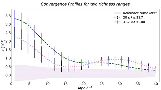
Convergence profiles for two richness ranges with its uncertainties. In green, the profile corresponding to sample S1. In pink, the profile corresponding to sample S3. It can be seen that the profiles differ significantly up to 15 Mpch−1, where the lower signal of sample S3 implies that the inclusion of low richness clusters produces a less significant convergence profile. A reference noise level from sample S1 for the CMB convergence map is shown in grey shaded region.
Given its larger signal, in what follows, we will consider this cluster richness threshold (samples S1 and S2, see Table 1 for details). In Fig. 4, we show mean κ profiles for two redshift ranges: 0.4 ≤ z < 0.45 (sample S1) and 0.45 ≤ z ≤ 0.5 (sample S2). As seen in this figure, the mean radial profiles obtained for the different redshifts bins are mutually consistent, in particular in the region up to 25 Mpch−1, as compared to the samples S1 and S3 that differ in richness. Also, it can be seen that the profile obtained for sample S2 has a more gentle decay than S1. We argue that these two behaviours are related to the different structures surrounding the cluster samples, influencing the radial profiles at large distances.
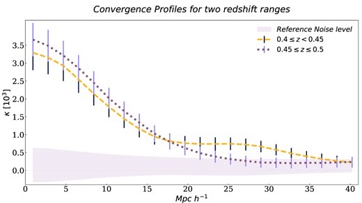
Convergence profiles for two redshift ranges with its uncertainties. In orange, the profile corresponding to sample S1. In violet, the profile corresponding to sample S2. It can be seen that both profiles have a reasonable agreement up to 25 Mpch−1. A reference noise level from sample S2 for the CMB convergence map is shown in grey shaded region.
In order to test the consistency of our results, we explore the convergence profiles of samples S1 and S2 in three different CMB lensing reconstructed maps using the PR3 MV, PR4 MV, and PR4 TT kLM coefficients. In Fig. 5, it can be seen the convergence profiles of these CMB lensing reconstructed maps compared to the convergence profile of the PR3 TT reconstructed map. Also it can be seen the corresponding statistical confidence regions. It can be noticed that in the PR3 release there is no difference between TT and MV reconstructed maps profiles. In addition, it can be inferred that there is no a statistically significant difference between the PR4 TT and MV profiles and the PR3 TT profile.
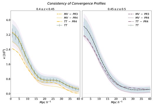
Consistency of the convergence profiles for samples S1 (yellow curves) and S2 (purple curves). The green solid line corresponds to the PR3 TT map. The dashed, dotted, and dash-dotted lines corresponds to PR3 MV, PR4 MV, and PR4 TT maps, respectively. 1σ (errorbar), 2σ (green shaded), and 3σ (pink shaded) variances corresponding to PR3 TT map are shown.
3.2 Oriented κ profiles
In order to derive κ profiles oriented along the cluster projected major axis, we use the same procedure as in Shin et al. (2018) and Gonzalez et al. (2021) to calculate the position angles of our cluster samples. We consider an uniform weight wk = 1 and all the galaxy members. Then we stack convergence map patches rotated according to these angles. The stacked aligned κ patches are shown in Fig. 6 for samples S1 and S2, respectively. For comparison, we also plot the non-aligned stacked patches. It can be seen that the κ distribution is preferentially oriented along the cluster major axis direction x after the clusters alignment. We notice the miscentring in sample S1, as well as a larger departure from a regular shape in S2. We argue that these two effects are mainly due to statistical fluctuations arising from both smoothing and large-scale irregularities in the mass distribution. This preferred alignment effect extends to several cluster radii up to 40 Mpch−1, which corresponds to ∼3°. In both cases, it can be seen that in the cluster nearby regions, <1°, the convergence is nearly isotropic unlike the outer regions where the convergence tends to show strongly elongated shapes. We also notice a low statistical significance beyond 2° (∼25 Mpch−1), as expected from the noise level of the convergence profiles in Figs 3 and 4.
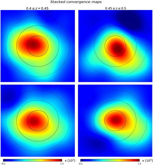
Stacked convergence maps for samples S1 (left-hand panels) and S2 (right-hand panels) with a smoothing corresponding to a FWHM Gaussian kernel of 2°, for a better visualization. The upper panels show the stacked maps without alignment. The lower panels show the stacked aligned maps. The black circles correspond to an angular scale of 1° (solid), 2° (dashed) and 3° (dotted). It can be seen in the aligned stacked maps that the convergence values are greater in the parallel orientation than in the perpendicular ones.
In order to highlight the alignment between the cluster orientation and the underlying mass distribution, we have computed the convergence profile for pixels within 45° from the cluster major axis direction, hereafter parallel direction. Similarly, we associate the perpendicular direction to the convergence profile for pixels with relative angles >45°. The resulting parallel and perpendicular convergence κ profiles for samples S1 and S2 are shown in Fig. 7. For reference, we also plot the total (parallel and perpendicular) radial profile shown and analysed in the previous section (see Fig. 4). The noise level corresponds to the radial profile. The vertical dotted line correspond to the virialized clusters region (∼3 Mpch−1) with a large κ uncertainty determination due to the presence of SZ imprint.
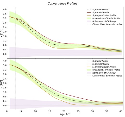
Convergence lensing parameter κ profile for sample S1 (upper panel) and S2 (lower panel) as a function of the projected distance to the cluster centres (black dotted line). Brown and yellow curves correspond to parallel and perpendicular directions as defined previously in the text, respectively. The green shaded region around the mean radial profile correspond to the radial uncertainty calculate through a bootstrap resampling technique with 300 re-samples from the considered sample. The horizontal grey shaded region is the map noise level calculated through 300 random profiles. The vertical dotted line represent two mean virial radius (∼3 Mpch−1), where a significant SZ effect is expected.
It can be seen that for both samples that the parallel profile has a significantly larger signal in a wide range of scales (from ∼5 to 40 Mpch−1) than the perpendicular ones. This behaviour is associated to the strong alignment between the inner non-linear virialized region (where the galaxy members use to calculate the position angles are located) and the large-scale mass distribution as provided by the convergence κ map. It is remarkable the fact that the alignment relates the distribution of galaxies, within ∼1–2 Mpch−1, and the mass density fluctuations at scales of at least 40 Mpch−1. This is particularly significant for the higher redshift bin (sample S2).
4 ANISOTROPIC LARGE-SCALE MASS DISTRIBUTION MODEL
In this section, we apply the anisotropic lensing model proposed by Gonzalez et al. (2022) to model the obtained κ convergence CMB data. The lensing effect produced by an ellipsoidal mass density can be studied through the surface mass density distribution Σ(R) with R the ellipsoidal radial coordinate R2 = r2(qcos2(θ) + sin2(θ)/q) with a semi-axis ratio q ≤ 1 (van Uitert et al. 2017). Following Schneider (1996), we define the ellipticity parameter |$\epsilon = \frac{1-q}{1+q}$| in order to obtain a multipolar expansion:
where θ is the relative position angle of the source with respect to the major axis of the density mass distribution. Σ0 y |$\Sigma _0^{\prime }$| are the monopolar and quadrupolar components, respectively. Σ0 is related to the axis-symmetrical mass distribution while the quadrupole component is defined in terms of the monopole as:
corresponding to an elongated mass distribution.
Based on the halo model, the total surface density distribution can be described according to the sum of a first and second halo components. The first halo term is modelled assuming a spherically symmetric NFW profile (Navarro, Frenk & White 1997), which can be parametrised by the radius that encloses a mean density equal to 200 times the critical density of the Universe, R200, and a dimensionless concentration parameter, c200:
where rs = R200/c200 is the scale radius, ρcrit is the critical density of the Universe, and δc is the characteristic overdensity described by:
We define M200 as the mass within R200 that can be obtained as:
To model this component, we consider the mean mass specified in Table 1, and we fix the concentration taking into account the relation given by Diemer & Joyce (2019) that is in agreement with the Simet et al. (2017) model for the mass calculation.
The tri-dimensional density profile of the second halo term is modelled considering the halo-matter correlation function, ξhm, as:
where ρm is the mean density of the Universe, satisfying:
and the halo-matter correlation function is related to the matter-matter correlation function through the halo bias (Seljak et al. 2005):
We set the halo bias by adopting Tinker et al. (2010) model calibration.
Thus, the radial surface density distribution can be modelled taking into account essentially the monopolar and quadrupolar terms (equation 7) of a main halo mass distribution, Σ1h, and a contribution to the mass from the cluster neighbourhood, Σ2h, corresponding to a second halo term, with independent ellipticity parameters:
This model assumes that the mass density distribution of the main halo, as well as the second halo term, are elongated along the same directions. Although a misalignment between the two haloes terms can exist, this expected misalignment will bias the estimated elongation of the second halo term to lower values.
We derive estimators of cluster mass and ellipticity from the convergence maps following the procedures detailed in Gonzalez et al. (2022) for the shear components. The model mass estimator arises from the integration of equation (13) on θ, which gives:
This estimator can be compared to the observed radial κ profile.
By multiplying equation (13) by cos(2θ) and integrating in θ, we obtain the model ellipticity estimators:
which is related with the anisotropic contribution and can be compared with the observed lensing effect, by averaging the convergence κ in angular bins:
In Fig. 8, we show the adopted model for the monopole (equation 15) together with the observed radial convergence profiles and the corresponding uncertainties. It can be seen the good behaviour of the model in the central range of distances [8, 40] Mpch−1 for the estimated mass derived from the richness–mass relation as a function of redshift for the redMaPPer clusters. It is worth noticing that our mass estimation through Simet et al. (2017) model is in agreement with that given in Geach & Peacock (2017; for details, see their fig. 3) in the richness range for samples S1 and S2.
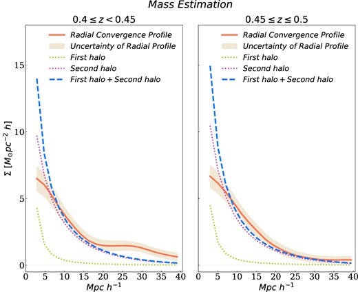
Density monopolar model compared to mean radial convergence profile for samples S1 (left-hand panel) and S2 (right-hand panel). In dashed blue, it can be seen the sum of the first halo term (dotted green) and second halo term (dotted pink) of the anisotropic density model calculated through 〈M〉 of samples S1 and S2. In orange, the mean radial convergence profiles with its uncertainty. It can be seen the good agreement of the model with respect to the measurements. The results on lower scales than 5 Mpch−1 have great statistical uncertainties and larger contamination of SZ effect.
The low-level agreement observed at small separations can be explained from the gaussian smoothing of the map and the low number of pixels in the first bins. Also, it is important to take into account that in these regions there exists a SZ effect that decreases the signal and may affect our measurements. Besides, we notice that this model aims at the analysis of weak lensing by clusters for both, observations (Gonzalez et al. 2021) and simulations (Gonzalez et al. 2022). Thus, several CMB lensing effects are not considered by this approach. Nevertheless, we acknowledge that the results are in a general good agreement in spite of the larger scales involved in our analysis.
We study the behaviour of the quadrupolar terms, which are derived from the monopolar ones (equation 8), and their respective ellipticities. With this aim, we fit the projected radial profile (equation 16) with respect to the ellipticity estimators (equation 15). Given that we neglect in our analysis the internal region which is sensitive to the main halo component, we fix the ellipticity for this term at ϵ1h = 0.2 that corresponds to a quasi-spherical halo shape and is in concordance with the previous redMaPPer ellipticity measurements (Shin et al. 2018; Gonzalez et al. 2021). Taking this into account, we use non-linear least squares to fit the second halo term that has the largest contribution to the surface density profile in the analysed radial range. We estimate the uncertainty in ϵ2h by means of the fitting covariance matrix. We notice that the estimated amplitude uncertainties are small, within the measurement errors, providing suitable associated ellipticity values. In Fig. 9, we show the resulting mean radial profile for the theoretical quadrupolar terms |$\epsilon _{1h}\Sigma _{1h}^{\prime }(r)$| and |$\epsilon _{2h}\Sigma _{2h}^{\prime }$| with ellipticities ϵ1h and ϵ2h for samples S1 and S2. As it can be seen in this figure, samples S1 and S2 have different second halo ellipticity parameter values being:
Given the different redshift depth of samples S1 and S2, we fix the corresponding fitting regions [10, 40], [17, 40] Mpch−1, respectively. We also notice that in the high redshift sample, the fit is less accurate than for sample S1, requiring a higher value of ϵ. We argue that these effects are caused by the strong alignment of the high redshift clusters at scales where there is still a significant convergence signal in the parallel direction.
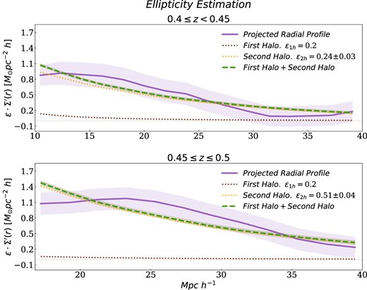
Fitting of the mean radial projected profile with respect to the anisotropic density quadrupolar model. In dashed green, it can be seen that the sum of the first halo term (dotted brown) and second halo term (dotted orange) of the anisotropic density model with ellipticities ϵ1h and ϵ2h. In violet, the mean radial projected profile and its uncertainties calculated through equation (16). For sample S1 (upper panel), the ellipticity parameters are ϵ1h = 0.2 and ϵ2h = 0.24 ± 0.03, corresponding to a quasi-spherical halo shape. For sample S2 (lower panel), the ellipticity parameters are ϵ1h = 0.2 and ϵ2h = 0.51 ± 0.04, which is related to a elongated halo shape. The grey shaded region shows the fitting uncertainty.
5 CONCLUSIONS
Due to its large angular extension and depth, there is a great potential in the investigations of CMB lensing map for the analysis of the mass distribution at large scales. These studies provide important alternative information to weak gravitational lensing research, involving shear estimations by background galaxies. In our work, we perform a statistical study of the convergence κ obtained from the temperature map of the CMB from the Planck 18 survey centred on rich galaxy clusters samples extracted from the redMaPPer catalogue. We find a significant excess in the convergence κ values around clusters, which extends several tens of Mpch−1. We study this κ profile for different richness samples as well as redshift intervals. We obtain, as expected, a larger amplitude for the higher richness samples and similar results for the redshift ranges explored. When clusters are aligned along their galaxy member distribution major axis, we find a significant difference between the κ values along the parallel and perpendicular directions. Remarkably, this difference persists at scales as large as 40 Mpch−1, indicating that this alignment is strongly conditioned by the large-scale mass anisotropic distribution. We study an anisotropic surface mass density model associated to the clusters, which is in reasonable agreement with the observational results obtained. From this analysis, we estimate the mean ellipticity of the second halo term for samples S1, ϵ2h = 0.24 ± 0.03 and S2, ϵ2h = 0.51 ± 0.04, consistent with an extended, highly flattened mass distribution oriented along the cluster major axis.
ACKNOWLEDGEMENTS
This work was partially supported by the Consejo Nacional de Investigaciones Científicas y Técnicas (CONICET), the Agencia Nacional de Promoción Científica y Tecnológica (PICT-2020-SERIEA-01404) and the Secretaría de Ciencia y Tecnología (SeCyT), Universidad Nacional de Córdoba, Argentina. Also, it was supported by Ministerio de Ciencia e Innovación, Agencia Estatal de Investigación and FEDER (PID2021-123012NA-C44). This work is based on observations obtained with Planck (http://www.esa.int/Planck), an ESA science mission with instruments and contributions directly funded by ESA Member States, NASA, and Canada. Some of the results in this paper have been derived using the healpix (Górski et al., 2005) package. Plots were made using python software and post-processed with inkscape.
DATA AVAILABILITY
The data underlying this article will be shared on reasonable request. The data sets used in this article were derived from sources in the public domain. Data products and observations from Planck, https://pla.esac.esa.int.
Footnotes
References
Author notes
Also at Port d’Informació Científica (PIC), Campus UAB, C. Albareda s/n, 08193 Barcelona (Barcelona), Spain.
