


ABSTRACT
Current observations of binary black hole (BBH) merger events show support for a feature in the primary BH-mass distribution at |$\sim \, 35 \ \mathrm{M}_{\odot }$|, previously interpreted as a signature of pulsational pair-instability supernovae (PPISNe). Such supernovae are expected to map a wide range of pre-supernova carbon–oxygen (CO) core masses to a narrow range of BH masses, producing a peak in the BH mass distribution. However, recent numerical simulations place the mass location of this peak above |$50 \ \mathrm{M}_{\odot }$|. Motivated by uncertainties in the progenitor’s evolution and explosion mechanism, we explore how modifying the distribution of BH masses resulting from PPISN affects the populations of gravitational-wave (GW) and electromagnetic (EM) transients. To this end, we simulate populations of isolated BBH systems and combine them with cosmic star formation rates. Our results are the first cosmological BBH-merger predictions made using the binary_c rapid population synthesis framework. We find that our fiducial model does not match the observed GW peak. We can only explain the |$35 \ \mathrm{M}_{\odot }$| peak with PPISNe by shifting the expected CO core-mass range for PPISN downwards by |$\sim {}15 \ \mathrm{M}_{\odot }$|. Apart from being in tension with state-of-the art stellar models, we also find that this is likely in tension with the observed rate of hydrogen-less super-luminous supernovae. Conversely, shifting the mass range upward, based on recent stellar models, leads to a predicted third peak in the BH mass function at |$\sim {}64 \ \mathrm{M}_{\odot }$|. Thus we conclude that the |$\sim {}35 \ \mathrm{M}_{\odot }$| feature is unlikely to be related to PPISN.
1 INTRODUCTION
The gravitational-wave (GW) observatories operated by the LIGO VIRGO KAGRA (LVK) collaboration have started to measure signals from GW mergers (LIGO Scientific Collaboration & Virgo Collaboration 2019; Abbott et al. 2021a), and with the recent release of the GWTC-3 there are now ∼90 confirmed compact object merger observations (Abbott et al. 2023; The LIGO Scientific Collaboration 2023), the majority of which are binary black hole (BBH) mergers. These observations show structure in the distribution of primary masses, Mprimary, i.e. the most massive object in the binary at the time of BBH merger. Parameteric models of the observations (e.g. Abbott et al. 2021b, 2023; Farah et al. 2023), as well as non-parametric models (e.g. Sadiq, Dent & Wysocki 2022; Callister & Farr 2023), consistently infer a feature, e.g. a change in power-law slope, or the presence of a Gaussian peak, between 32 and |$38 \ \mathrm{M}_{\odot }$|, suggesting that this feature is robust. The exact nature and origin of this feature is unclear, but the often-proposed explanation is that it originates from a pile up of BH masses due to pulsational pair-instability supernovae (PPISNe; Talbot & Thrane 2018; Stevenson et al. 2019; Belczynski et al. 2020; Karathanasis, Mukherjee & Mastrogiovanni 2023). However, several alternative explanations for such a feature have also been proposed (e.g. Li et al. 2022; Antonini et al. 2023; Briel, Stevance & Eldridge 2023).
PPISNe occur when a very massive star is dynamically unstable due to runaway electron-positron pair-formation in their cores which remove high-energy photons. This leads to a decrease in the radiation pressure and an increase of the mass-density, and causes a softening of the equation of state, i.e. a decrease of the adiabatic index. The process results in an initial collapse, the explosive ignition of oxygen in the core, and a subsequent pulsating behaviour through which the star loses mass, or a single violent explosion that leaves behind no remnant (Barkat, Rakavy & Sack 1967; Rakavy & Shaviv 1967; Woosley, Blinnikov & Heger 2007; Woosley 2017; Marchant et al. 2019; Renzo et al. 2020b, a; Farmer et al. 2020; Farag et al. 2022). PPISNe cause a wide range of pre-supernova core masses to form BHs in a narrow range of remnant masses, which leads to an over-density and a subsequent mass-gap at higher BH masses. The magnitude of this over-density, or pile-up, depends on the width of the pre-supernova core-mass range that undergoes PPISN and consequently on how sensitive the PPISN mass-loss is to the pre-supernova core mass. A broader pre-supernova core-mass range, i.e. a shallower PPISN remnant mass curve, leads to a larger pile-up.
Detailed models of single stars allow estimates of the mass lost during the pulsations at a given helium (He) or carbon–oxygen (CO) core mass (Renzo et al. 2022). These are used to calculate an upper limit on the BH remnant mass that can form after subsequent core-collapse (CC) supernovae (Farmer et al. 2019, from hereon F19; Farag et al. 2022) and the location of a feature in the primary-mass distribution due to PPISNe which is consistently predicted at masses |$\gtrsim {}40-45 \ \mathrm{M}_{\odot }$| (Talbot & Thrane 2018; Stevenson et al. 2019; Belczynski et al. 2020). This mass is significantly (|$\gtrsim {}5 \ \mathrm{M}_{\odot }$|) greater than the |$\sim {}35 \ \mathrm{M}_{\odot }$| location of the feature inferred from GW data. Moreover, it is remarkably robust against the most common uncertainties in massive stellar evolution, such as metallicity, mixing, and neutrino physics (Farmer et al. 2019).
However, there are uncertainties that lead to larger variations in the mass range and remnant mass of stars that undergo PPISN. Several processes have been suggested that lead to shifts in the CO-core masses that undergo PPISN. These include uncertainties in the nuclear burning rates that affect the carbon-to-oxygen (C/O) ratio in the core (deBoer et al. 2017; Farmer et al. 2019, 2020; Costa et al. 2021; Woosley & Heger 2021; Mehta et al. 2022; Farag et al. 2022; Shen et al. 2023), rotation, which provides both more massive cores and enhanced dynamical stability (Glatzel, Fricke & El Eid 1985; Maeder & Meynet 2000; Chatzopoulos & Wheeler 2012; Marchant & Moriya 2020), beyond Standard Model physics which can either affect the C/O ratio (Croon, McDermott & Sakstein 2020), or lead to reduced dynamical stability (Croon et al. 2020; Sakstein, Croon & McDermott 2022; Mori et al. 2023) at lower masses, and lastly dark-matter annihilation which acts like an additional heating source (Ziegler & Freese 2021, 2022). These processes could lower the CO core masses that undergo PPISN by up to |$-20 \ \mathrm{M}_{\odot }$| (axion instability) or increase them by up to |$+10 \ \mathrm{M}_{\odot }$| (reaction rates, rotation). Moreover, some theoretical studies predict additional mass loss, either in the post pulsational pair-instability (PPI) CC due to changes in core structure of PPI stars affecting the propagation of the core-bounce shock (Marchant et al. 2019; Renzo et al. 2020b; Powell, Müller & Heger 2021; Rahman et al. 2022), or by how convection transports energy during the PPI (Renzo et al. 2020a). Furthermore, recent SN observations are well modelled by post-PPI mass loss (Ben-Ami et al. 2014; Kuncarayakti et al. 2023; Lin et al. 2023). Both theoretical studies and observational estimates find, at most, |$10 \ \mathrm{M}_{\odot }$| in additional mass loss.
The location of the pair-instability supernova (PISN) mass-gap has broad implications. If the high-mass feature at |$\sim {}35 \ \mathrm{M}_{\odot }$| is indeed caused by PPISN, it observationally constrains the maximum BH mass that stars can form below the full disruption by PISN, and thus the lower bound of the so-called PISN mass-gap (Woosley, Heger & Weaver 2002; Renzo et al. 2020b; Woosley & Heger 2021). Only stars with He-core masses |$\gtrsim {}120 \ \mathrm{M}_{\odot }$| at the onset of collapse, which experience photo-dissociation during the pair-instability, can directly collapse into more-massive BHs (Bond, Arnett & Carr 1984; Renzo et al. 2020b; Siegel et al. 2022). The PISN mass-gap further helps determine the fractional contribution of different GW source channels to the overall population of BBH mergers, because systems with masses in the gap originate from channels other than isolated-binary evolution (Arca Sedda et al. 2020; Baibhav et al. 2020; Safarzadeh 2020; Wong et al. 2021). The location of the mass gap also constrains stellar physics, like the aforementioned uncertain nuclear reaction rates 12C(α, γ)16O and 3α (Farmer et al. 2019; Farag et al. 2022; Mehta et al. 2022; Shen et al. 2023). Lastly, the location of the mass-gap and the pile-up may be redshift independent sign-posts for cosmological applications (Farr et al. 2019, and references therein).
One way to constrain the physics of PPISNe is to compare our simulations directly to the observed rate of electromagnetic (EM) transients. Unfortunately, unambiguous transient observations of PPISN are currently not available. Theoretical modelling of PISNe light curves show that their light curves generally rise slowly and that some are very luminous at peak luminosity (Kozyreva et al. 2014), while those caused by PPISNe and the subsequent interaction of their ejecta with the circumstellar medium or previously ejected mass-shells (Moriya & Langer 2015; Woosley 2017; Renzo et al. 2020b) have shorter rise-times but equally high peak luminosities (Woosley et al. 2007). Some super-luminous supernovae (SLSNe) could be powered by either PISNe or PPISNe, and indeed some of these are suggested observations of PISNe or PPISNe (e.g. Lunnan et al. 2018; Aamer et al. 2023; Lin et al. 2023; Schulze et al. 2023), although as of yet none of them have been confirmed to be caused by either PISNe or PPISNe. Moreover, there is growing evidence from light curves, spectra and rates that not all SLSNe are powered by PISNe or PPISNe (Nicholl et al. 2013; Kozyreva & Blinnikov 2015; Perley et al. 2016; Gilmer et al. 2017). Estimates of (P)PISN event-rate densities are useful to study stellar evolution (e.g. du Buisson et al. 2020; Briel et al. 2022; Tanikawa et al. 2023), and could be compared to SLSN rates to determine whether these rates are in tension (Nicholl et al. 2013). Although uncontroversial detections are lacking, there are debated candidates for both PISNe and PPISNe, e.g. SN 1961V (Woosley & Smith 2022), SN 1000 + 0216 (Cooke et al. 2012), SN 2010mb (Ben-Ami et al. 2014), PTF10mnm (Kozyreva et al. 2014), iPTF14hls (Wang et al. 2022), iPTF16eh (Lunnan et al. 2018), SN 2016iet (Gomez et al. 2019), SN 2017egm (Lin et al. 2023), SN 2018ibb (Schulze et al. 2023), and SN 2019szu (Aamer et al. 2023). However, their interpretation is sufficiently uncertain that estimating a rate from these observations is still a challenge (however, see also Nicholl et al. 2013).
In this study we explore how the remnants of PPISNe affect the distribution of Mprimary for the BBH systems merging at redshift z ∼ 0.2, and compare this primary-mass distribution to the current observations. We focus our results on redshift z ∼ 0.2 because this is where current observations provide the strongest constraints (Abbott et al. 2023). We evolve isolated binary systems and convolve the resulting BBH systems with recent star formation rate (SFR) prescriptions (van Son et al. 2022a), combined with a new PPISNe remnant-mass prescription (Renzo et al. 2022). We introduce variations in this prescription to capture the effects of uncertain or new physics. Moreover, we estimate the rates of PPISNe and PISNe and compare them to the observed SLSNe to constrain our variations. We aim to evaluate whether the peak at |$35 \ \mathrm{M}_{\odot }$| is explained by BHs formed through PPISNe.
The layout of this paper is as follows. In Section 2 we explain our method to simulate populations of BBHs through population synthesis (Sections 2.1 and 2.2) and describe our approach to convolving our binary populations with SFRs (Section 2.3). In Section 3 we explain our variations of the PPISN mechanism. In Section 4 we show the primary-mass distributions at z = 0.2, and BBH merger and EM transient event-rate densities as a function of redshift in our fiducial populations and the populations with variations on the PPISNe mechanism. We discuss our findings and conclude in Sections 5 and 6.
2 METHOD
We simulate populations of binary-star systems using binary_c, a binary population-synthesis framework based on the stellar-evolution algorithm of Hurley, Pols & Tout (2000) and Hurley, Tout & Pols (2002), which makes use of the single-star models of Pols et al. (1998) and provides analytical fits to their evolution as in Tout et al. (1997) with updates in Izzard et al. (2004, 2006, 2009, 2018), Claeys et al. (2014), Izzard & Jermyn (2022), and Hendriks & Izzard (2023).
We combine the results of these populations with cosmological SFRs, similar to, e.g. Dominik et al. (2013, 2015), Belczynski et al. (2016), Mandel & de Mink (2016), Chruslinska, Nelemans & Belczynski (2019), Neijssel et al. (2019), van Son et al. (2022a), and Tanaka et al. (2023) to estimate the rate and mass distribution of merging BBH systems as a function of redshift.
2.1 Population synthesis and input physics
For an in-depth review of the relevant physical processes in binary stellar physics, see Langer (2012), Postnov & Yungelson (2014), De Marco & Izzard (2017), and Petrović (2020). We highlight our choices of physics prescriptions for the processes relevant to this study in the following sections.
2.1.1 Mass transfer, stability, and common-envelope evolution
During their evolution, stars in binary systems interact with their companion by expanding and overflowing their Roche–Lobe, resulting in mass flowing from the donor star to its companion. We take the mass-transfer rate of the donor from Claeys et al. (2014). When the accretor has a radiative envelope, we limit the mass-accretion rate to 10-times its thermal limit, |$\dot{M}_{\mathrm{acc\ thermal\ limit}} = 10\, \dot{M}_{\mathrm{KH,\ acc}}$|, where |$\dot{M}_{\mathrm{KH,\ acc}} = M_{\mathrm{acc}}/\tau _{\mathrm{KH}}\ \mathrm{M}_{\odot }\, \mathrm{yr}^{-1}$| with τKH the global Kelvin–Helmholtz time-scale of the accretor and the factor of 10 roughly accounts for the fact that initially only the outer envelope, which has a shorter time-scale than the global τKH, responds to mass accretion. We do not similarly limit the accretion rate of giant-type stars with convective envelopes because we assume that they shrink in response to mass accretion (Hurley et al. 2002). We do not expect this assumption to have a dominant impact because, over all redshifts, only up to 10 per cent of the merger rate of our BBH mergers consists of systems that undergo any episode of mass transfer onto a giant-like star. We further limit the accretion rate onto compact objects by the Eddington accretion rate limit. We assume any mass transfer exceeding the accretion rate limits is lost from the system. Moreover, we assume that that mass carries a specific angular momentum equal to the specific orbital angular momentum of the accretor, the so-called isotropic re-emission mass loss (Soberman, Phinney & van den Heuvel 1997). We calculate the stability of mass transfer based on the critical mass ratio, qcrit = Maccretor/Mdonor, at the onset of mass transfer. For stars on the main sequence, Hertzsprung gap, giant branch, early asymptotic giant branch (AGB) and thermally pulsing AGB we use the qcrit of Ge et al. (2015, 2020). For the remaining stellar types we use the qcrit of Claeys et al. (2014).
Recent studies suggest that the rate of BBH mergers that experience and survive common-envelope (CE) evolution might be overestimated (Marchant et al. 2016; Klencki et al. 2021; Gallegos-Garcia et al. 2021; Olejak, Belczynski & Ivanova 2021), and they argue that mass transfer should either generally be more stable or the ejection of the envelope much more difficult and hence the stars merge (see, however, Renzo et al. 2023). Independently, both van Son et al. (2022b) and Briel et al. (2023) showed that the CE channel is not necessary to explain the rate of BBH mergers, while the converse is true for binary neutron-star mergers (Chruslinska et al. 2018; Tanaka et al. 2023). More importantly, van Son et al. (2022a) shows that high-mass BBH systems are almost exclusively formed through the stable mass-transfer channel, and that the CE channel is inefficient for the formation of systems with |$M_{\mathrm{primary}}\gt 25 \ \mathrm{M}_{\odot }$|. Other population synthesis studies like Belczynski et al. (2022; startrack), Mapelli et al. (2019, 2022; mobse), and Briel et al. (2023; bpass) come to the same conclusion. In this work we test this with binary_c and find the same results (Section 4.1 and Appendix B). Therefore, we focus on the stable mass-transfer channel and generally exclude merging systems that survive a CE (indicated with ‘excluding CE’) from our primary mass distribution results and our merger rate densities unless explicitly indicated with ‘including CE’ (see also Fig. B1).
2.1.2 Wind mass loss
We follow Schneider, Podsiadlowski & Müller (2021) in our choice of wind mass loss prescriptions, with the exception of their LBV-wind prescription. For hot-star (|$T_{\mathrm{eff}} \gt 1.1\, \times \, 10^{4}$| K) winds we use the prescriptions from Vink, de Koter & Lamers (2000), Vink, de Koter & Lamers (2001). For Wolf-Rayet star wind mass loss we use the prescription of Yoon (2017). For low-temperature (Teff < 104 K) stellar winds we use Reimers (1975) mass loss on the first giant branch, with η = 0.4, and Vassiliadis & Wood (1993) on the AGB. At intermediate temperatures we linearly interpolate. Beyond the Humphreys-Davidson limit (Humphreys & Davidson 1994) we use the prescription for LBV-winds as described in Hurley et al. (2000). We do not include the effects of rotationally enhanced mass loss.
2.1.3 Neutrino loss during compact object formation
For stars that only experience a CCSN we calculate the baryonic remnant mass, Mrem, bary, using the delayed prescription of Fryer et al. (2012). We calculate the gravitational remnant mass, Mrem, grav, of BHs formed through PPISNe and CCSNe from
(Zevin et al. 2020). Equation (1) reduces the compact-object mass because of loss of neutrinos during the collapse of the star. Because even in extremely massive stars the CC releases a few 1053–1054 erg in neutrinos, we limit this correction to |$0.5 \ \mathrm{M}_{\odot }{}\simeq {}10^{54} \ \mathrm{erg} \, c^{-2}$| (Aksenov & Chechetkin 2016; Zevin et al. 2020; Rahman et al. 2022).
2.1.4 Envelope ejection following neutrino losses
During CC, rapid changes in core mass because of neutrino emission change the potential energy of a star, and lead to a pressure wave travelling outward. This pressure wave, in some cases, evolves into a shock wave. In stars with low envelope binding energy (>−1048 erg), like red super giants, this leads to a loss of (part of) the outer envelope (Nadezhin 1980; Lovegrove & Woosley 2013; Piro 2013). Because the expected mass loss depends on the structure of the core and the binding energy of the envelope, most mass is lost from red (super) giants. Stars with compact envelopes, such as blue and yellow super giants or Wolf–Rayet stars, are not expected to lose much mass (Fernández et al. 2018; Ivanov & Fernández 2021). We thus apply this effect only to red (super) giants when the explosion is expected to fail (i.e. ffallback = 1), and assume that everything outside the He core is lost,
where ΔMν, env is the ejected mass due to neutrino loss, Mtot is the total mass of the star, and MHe is the mass of its He core. We assume this mass is ejected symmetrically and does not introduce a natal kick to the star, other than a ‘Blaauw’ kick (Blaauw 1961), due to the change in centre of mass. We do not apply this mass loss term to blue and yellow supergiants and Wolf–Rayet progenitors. In cases where the explosion is successful, the matter that may be ejected because of the neutrino losses would anyway be easily removed by the SN shock (as accounted for by the delayed) therefore we do not need to apply equation (2) when ffallback < 1.
2.1.5 Supernova natal kick
Stars that undergo CC may receive a natal momentum kick due to asymmetries in the resulting explosion (Shklovskii 1970; Fryer 2004; Janka 2013; Grefenstette et al. 2016; Holland-Ashford et al. 2017; Katsuda et al. 2018). We calculate the supernova kick by sampling a kick speed, |$V_{\mathrm{sampled\, kick}}$| from a Maxwellian distribution with dispersion of |$\sigma _{\mathrm{kick}} = 265 \ \mathrm{km\, s^{-1}}$| and sampling a direction isotropically on a sphere (Hobbs et al. 2005). We scale the natal kick speed with the fallback fraction, ffallback = Mfallback/MSNejecta, where Mfallback is the total mass that falls back onto the remnant and MSNejecta is the initial total supernova ejecta as
We calculate this fraction through the delayed CCSN prescription of Fryer et al. (2012). In Appendix C we discuss a different scaling. Moreover, even if the supernova ejecta do not impart a natal kick, as long there is any mass ejected, the system still experiences a Blaauw kick. In PPISNe we assume spherically symmetric ejecta, and no natal kick other than the Blaauw kick (Chen et al. 2014, 2022; Chen, Woosley & Whalen 2020).
2.2 Simulated populations
Binary-star systems are characterized by their initial primary mass, M1, secondary mass, M2, orbital period, P, eccentricity, e, and metallicity, Z. To evolve a population of binary systems, we vary each of these initial properties by sampling from their probability distributions. In this study we assume all the probability distributions are separable and can be calculated independently.
For the initially more massive star (primary mass, M1) we assume an initial mass function (IMF) of Kroupa (2001). We sample NM1 stars between 7.5 and |$300 \ \mathrm{M}_{\odot }$|. Stars of an initially lower mass do not form BHs and we do not include these in our populations. We sample the initially less-massive star from a flat distribution in q = M2/M1 (Sana et al. 2012) between 0.08/M1 and 1, with a resolution Nq. We sample the orbital period |$P_{\mathrm{\mathrm{orb}}}$| of the binary systems from a logarithmically spaced distribution between 0.15 and 5.5 |$\mathrm{log}_{10}\left(\, P_{\mathrm{orb}}/\mathrm{d}\right)$|, with the distribution function from Kobulnicky & Fryer (2007) for systems with a primary mass below |$15 \ \mathrm{M}_{\odot }$| and the power-law in |$\mathrm{log}_{10}\left(\, P_{\mathrm{orb}}/\mathrm{d}\right)$| distribution function with exponent 0.55 from Sana et al. (2012) for systems with |$M_{1} \gt 15 \ \mathrm{M}_{\odot }$|. We neglect the possibility of initially eccentric binaries because with the tidal circularisation model of Hurley et al. (2002) that we employ, they all circularise before interaction (de Mink & Belczynski 2015).
We assign a probability, pi, to each system, i, which is a product of the probability density functions of each variable and the step size in phase space, see Izzard & Halabi (2018) for a detailed explanation of the method. Appendix D shows how we use the probabilities pi and the binary fraction fbin in our merger-rate calculation. Throughout this study we assume a constant binary fraction fbin = 0.7.
We use a resolution of NM1 = 750 for our single-star system parameter distributions. We use a resolution of NM1 = 75, Nq = 75, NP = 75 for our binary-system parameter distributions. We simulate NZ = 12 populations of single and binary systems, with metallicity equally spaced in log10(Z) between log10(Z) = −4 (corresponding to very metal-poor stars with negligible wind mass-loss) and log10(Z) = −1.6 (corresponding to super-solar stars with strong wind mass loss). At each supernova we sample the natal kick direction and magnitude (Section 2.1.5) NSN kick = four-times, and divide the probability fraction of the system as pi/NSN kick. This amounts to an initial total of |$\sim {}4\, \times \, 10^{5}$| binaries at each metallicity, of which a subset splits due to multiple kick samples.
2.3 Cosmological star formation history
We calculate the intrinsic redshift-dependent merger-rate density of BBH systems, |$\mathcal {R}_{\mathrm{BBH}}(z_{\mathrm{merge}},\ \zeta)$|, merging at redshift zmerge, or the corresponding merging lookback time, |$t^{*}_{\mathrm{merge}}$|, with a set of system properties, ζ, (e.g. orbital period, primary mass, metallicity) similarly to the compas code (Neijssel et al. 2019; Broekgaarden et al. 2021; Riley et al. 2022; van Son et al. 2022a). We define the intrinsic redshift-dependent merger-rate density as
The integrand consists of the number of BBH systems per formed solar mass, |$\mathcal {N}_{\mathrm{form}}(Z,\, t_{\mathrm{delay}},\, \zeta)$|, as a function of metallicity Z, delay time, tdelay, and system properties, ζ, and the SFR density, SFR(Z, zbirth), as a function of Z and the birth redshift, zbirth. The delay time, tdelay, is the sum of the time it takes from the systems birth to the moment the second BH forms (DCO formation), tform, and the time it takes the DCO to inspiral and merge due to emission of GW radiation, tinspiral. The inspiral time tinspiral of the BBH system is computed from Peters (1964). The birth redshift corresponds the birth lookback time of the system, |$t^{*}_{\mathrm{birth}} = t^{*}_{\mathrm{merge}} + t_{\mathrm{delay}}$|. Generally, times with a * superscript are lookback times and those without are durations. We integrate this over metallicity between the metallicity bounds Zmin and Zmax (Section 2.2), and over the delay time tdelay between 0 and |$t^{*}_{\mathrm{first\, SFR}}-t^{*}_{\mathrm{merge}}$| to avoid integrating beyond |$t^{*}_{\mathrm{first\, SFR}}$|, which is the lookback time of first star-formation and has the corresponding first star-formation redshift |$z_{\mathrm{first\, SFR}}$|.
We determine |$\mathcal {N}_{\mathrm{form}}(Z,\, t_{\mathrm{delay}},\, \zeta)$| by simulating populations of binary stars (Section 2.2 and Appendix D) with primary stars between 7.5 and |$300 \ \mathrm{M}_{\odot }$|, and we convolve BBH systems with the SFR(z, Z) of van Son et al. (2022a), with redshifts between 0 and zFirst SFR = 10 and a step size of dz = 0.025 through the discretized version of equation (4). We use the PLANCK13 (Ade et al. 2014) cosmology to calculate redshift as a function of the age of the universe and the volume spanned by the redshift shells.
To calculate the total merger-rate density at a given redshift we integrate equation (4) over all system properties ζ,
While the total merger rate is degenerate in both the adopted cosmology/SFR prescription and the adopted stellar physics (e.g. Broekgaarden et al. 2022), the locations of the features in the mass distribution of merging BBHs are robust under the uncertainties of the SFRs (van Son et al. 2023). In this study we therefore fix the SFR prescription and only vary the prescription for PPISNe.
3 THE PPISN REMNANT MASS PRESCRIPTION AND ITS VARIATIONS
We model the mass loss of (P)PISNe with the prescription of Renzo et al. (2022), which is based on the detailed models of F19. This prescription takes a ‘top-down’ approach, that is it prescribes the total mass lost for a given CO core mass, rather than directly prescribes a remnant mass. This allows us to incorporate all possible mass-loss mechanisms when compact objects with masses above and below the PPISN regime form without introducing artificial jumps in the remnant mass function. We show an example pre-SN core to remnant-mass relation for our fiducial model at metallicity Z = 0.001 in Fig. 1. F19 also provide a remnant-mass prescription based on their detailed models which we include in our study. We call this the F19 model.
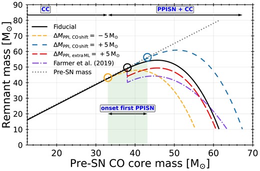
Remnant mass vs. pre-SN CO core mass in single stars at metallicity Z = 0.001. The grey dotted line shows the pre-SN mass, the black line shows the remnant mass with our fiducial implementation (Renzo et al. 2022), and the purple dash–dotted line shows the remnant mass as given by the prescription of F19. The dashed coloured lines indicate example variations on the PPISNe prescription. The orange-dashed line indicates a downward CO core-mass shift of |$\Delta M_{\mathrm{PPI,\, CO\, shift}}= -5 \ \mathrm{M}_{\odot }$|, the red long-dashed line indicates an additional mass loss of |$\Delta M_{\mathrm{PPI,\, extra\, ML}}= +5 \ \mathrm{M}_{\odot }$|, and the blue loosely dashed line indicates an upward CO core-mass shift of |$\Delta M_{\mathrm{PPI,\, CO\, shift}}= +5 \ \mathrm{M}_{\odot }$|. The corresponding circles indicate the CO core mass of the PPISN onset for each variation. The green shaded region indicates the range of PPISNe onset CO core masses spanned by the example variations.
We assume that stars with a minimum CO core mass |$M_{\mathrm{CO,\ Min,\ PPISN}} = 38 \ \mathrm{M}_{\odot }$| after carbon burning undergo PPISNe. If pulsations lead to a remnant mass below |$10 \ \mathrm{M}_{\odot }$| we regard the supernova as a PISN which leaves no remnant behind (Marchant et al. 2019). For CO core masses greater than |$114 \ \mathrm{M}_{\odot }$| we assume direct collapse to a BH following the photodisintegration instability (Bond et al. 1984; Renzo et al. 2020b). If, at the onset of pulsations, the star still has a hydrogen-envelope, we assume this is always expelled, and the hydrogen envelope mass is added to the prescribed mass loss due to pulsations (appendix B, Renzo et al. 2020b).
In Section 1 we mention several processes that introduce a large uncertainty in CO core masses that undergo PPI compared to our fiducial model. This motivates us to consider introducing a parameter to shift the CO core-mass range that undergoes PPI in our prescription. Moreover, the observational (Ben-Ami et al. 2014; Kuncarayakti et al. 2023; Lin et al. 2023) and theoretical (Powell et al. 2021; Rahman et al. 2022) indications of additional post-PPI mass-loss motivates us to consider this in our prescription as well.
We capture these effects by modifying our prescription from Renzo et al. (2022) to allow such variations and hence our predicted PPISNmass loss is
where |$\Delta M_{\mathrm{PPI,\, CO\, shift}}$| is the mass by which we shift the CO core-mass requirement for PPISNe. Negative |$\Delta M_{\mathrm{PPI,\, CO\, shift}}$| shifts the core-mass range to lower masses, and vice-versa. |$\Delta M_{\mathrm{PPI,\, extra\, ML}}$| represents additional, post-pulsation, mass loss, and Z is the metallicity of the star.
We vary |$\Delta M_{\mathrm{PPI,\, CO\, shift}}$| between |$-20 \ \mathrm{M}_{\odot }$| and |$+10 \ \mathrm{M}_{\odot }$|, and |$\Delta M_{\mathrm{PPI,\, extra\, ML}}$| between |$0 \ \mathrm{M}_{\odot }$| and |$+20 \ \mathrm{M}_{\odot }$|, in steps of |$5 \ \mathrm{M}_{\odot }$|. We note that |$\Delta M_{\mathrm{PPI,\, CO\, shift}}= +10 \ \mathrm{M}_{\odot }$| qualitatively behaves like Farag et al. (2022) and |$\Delta M_{\mathrm{PPI,\, CO\, shift}}= -15 \ \mathrm{M}_{\odot }$| behaves qualitatively like the f = 0.5 model of Mori et al. (2023), corresponding to an axion mass of half the electron mass.
Varying |$\Delta M_{\mathrm{PPI,\, CO\, shift}}$| and |$\Delta M_{\mathrm{PPI,\, extra\, ML}}$| allows us to determine how a shift of the PPISN CO core-mass range or additional mass loss from PPISNe affects the remnant-mass distribution, and specifically whether these changes lead to a feature in the primary-mass distribution at |$\sim {}35 \ \mathrm{M}_{\odot }$|.
Fig. 1 shows an example of the remnant-mass distribution as a function of the pre-SN CO core mass at Z = 0.001 with a CO core mass shift of |$\Delta M_{\mathrm{PPI,\, CO\, shift}}= \pm 5 \ \mathrm{M}_{\odot }$|. The shift of the range of CO core masses that undergo PPISN both affects the (P)PISNe as well as CCSNe. By shifting the range to lower or higher masses, the CO core masses that undergo CC decrease or increase, respectively. It is important to note that a translation in the CO core mass that undergoes PPISN does not translate directly to the same shift in ZAMS masses. This difference is caused by a non-linear relation between the ZAMS mass and the pre-SN CO core mass (e.g. Limongi & Chieffi 2018). In Appendix A we show examples of the dependence of the remnant mass as a function of ZAMS mass and metallicity.
We further note that additional mass loss (|$\Delta M_{\mathrm{PPI,\, extra\, ML}}$|) only affects stars that already undergo PPISNe. Hence it does not affect the rate of CCSNe but only the rate of, and ratio between, PPISNe and PISNe, because too much additional mass loss turns a PPISN into a PISN. Another effect of our implementation is that at high additional mass loss (|$\Delta M_{\mathrm{PPI,\, extra\, ML}}\gt 10$|), the most massive BH formed through single-star evolution is from direct CC, not through PPISN + CC. We show how |$\Delta M_{\mathrm{PPI,\, extra\, ML}}= 10 \ \mathrm{M}_{\odot }$| affects the initial-final-mass relation in a grid of masses and metallicities Appendix A.
4 RESULTS
In this section we present the results of our simulations. We present the primary BH-mass distributions of our models with varying PPISNe mechanism properties in Section 4.1 and the event-rate densities of EM-transient events as well as GW-merger events in Section 4.2. We emphasize that in Section 4.1 we exclude systems that undergo CE evolution. See Section 2.1.1 for our motivation and Appendix B for results that include CE evolution.
4.1 Primary-mass distributions
We show the primary-mass distribution of merging BBHs for our CO core-mass shift models, |$\Delta M_{\mathrm{PPI,\, CO\, shift}}$| and our additional mass loss models, |$\Delta M_{\mathrm{PPI,\, extra\, ML}}$|, in Figs 2 and 3. Panels 2(a) and 3(a) show the merger-rate density of BBH systems as a function of primary-BH mass. Panels 2(b) and 3(b) show the fraction of primary-mass BHs that are formed through PPISNe.
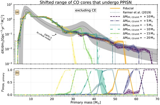
Panel (a): Merger rate density as a function of primary mass for BBH mergers at z = 0.2, for our fiducial model (orange solid), the F19 model (grey dotted), and our CO core-mass shift variations |$\Delta M_{\mathrm{PPI,\, CO\, shift}}= +10 \ \mathrm{M}_{\odot }$| (dark-purple dashed), |$\Delta M_{\mathrm{PPI,\, CO\, shift}}= +5 \ \mathrm{M}_{\odot }$| (blue dash–dotted), |$\Delta M_{\mathrm{PPI,\, CO\, shift}}= -5 \ \mathrm{M}_{\odot }$| (light-blue dotted), |$\Delta M_{\mathrm{PPI,\, CO\, shift}}= -10 \ \mathrm{M}_{\odot }$| (dark-green long-dashed) |$\Delta M_{\mathrm{PPI,\, CO\, shift}}= -15 \ \mathrm{M}_{\odot }$| (green dashed), and |$\Delta M_{\mathrm{PPI,\, CO\, shift}}= -20 \ \mathrm{M}_{\odot }$| (yellow long dash–dotted). The lines connect the centres of the bins (stepped) of width |$2.5 \ \mathrm{M}_{\odot }$|. The translucent bands around the lines are the regions of 90 per cent confidence-intervals obtained by 50 bootstrap samples of the double compact-object (DCO) populations. The dark-grey line indicates the mean of the power law + peak model of Abbott et al. (2023) at z = 0.2 and the grey shaded region indicates the 90 per cent confidence interval. These models indicate that the fiducial model does not peak at the observed location, and we need to introduce a shift of as much as |$\Delta M_{\mathrm{PPI,\, CO\, shift}}= -15 \ \mathrm{M}_{\odot }$| to make the distribution peak at the observed mass. The upward shift of |$\Delta M_{\mathrm{PPI,\, CO\, shift}}= +10 \ \mathrm{M}_{\odot }$| that matches Farag et al. (2022) forms a slight over-density at |$\sim 64 \ \mathrm{M}_{\odot }$|. Panel (b): Fraction of systems in that bin where the primary BH formed through PPISN.
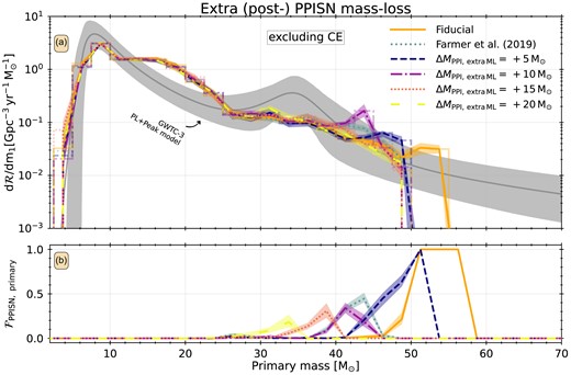
As Fig. 2 for our fiducial model (orange solid), the F19 model (grey dotted), and our additional mass loss models |$\Delta M_{\mathrm{PPI,\, extra\, ML}}= 5 \ \mathrm{M}_{\odot }$| (dark-blue dashed), |$\Delta M_{\mathrm{PPI,\, extra\, ML}}= 10 \ \mathrm{M}_{\odot }$| (purple dash–dotted), and |$\Delta M_{\mathrm{PPI,\, extra\, ML}}= 15 \ \mathrm{M}_{\odot }$| (red dotted), |$\Delta M_{\mathrm{PPI,\, extra\, ML}}= 20 \ \mathrm{M}_{\odot }$| (yellow long-dashed). These models indicate that additional mass loss models lower the merger rate density of systems with |$M_{\mathrm{primary}}\gt 48 \ \mathrm{M}_{\odot }$|, and for some models (|$\Delta M_{\mathrm{PPI,\, extra\, ML}}= 5 \ \mathrm{M}_{\odot }$| and |$\Delta M_{\mathrm{PPI,\, extra\, ML}}= 10 \ \mathrm{M}_{\odot }$|) increases the rate between Mprimary = 40 and |$48 \ \mathrm{M}_{\odot }$|, forming a peak. Below |$40 \ \mathrm{M}_{\odot }$| the primary mass distribution is not affected by any amount of additional mass loss.
Our fiducial primary-mass distribution at redshift z = 0.2 (Fig. 2a, orange line) peaks at about |$10 \ \mathrm{M}_{\odot }$| in good agreement with the LVK observations (Abbott et al. 2023). Moreover, in the intermediate range of 12 < Mprimary/M⊙ < 25 we predict more mergers than observed, which is seen in several binary star evolution (bse; Hurley et al. 2002)-based rapid population-synthesis codes (e.g. Mapelli et al. 2022; van Son et al. 2023), though the origin of this over-production is unknown. This region contains systems that undergo at least one stable mass-transfer episode and we do find indications that the mass-transfer stability prescriptions affect the width and height of this over-density. Additionally, we find that among systems with |$M_{\mathrm{primary}}\gt 12 \ \mathrm{M}_{\odot }$| some merge without undergoing any mass transfer but are able to merge because they form with very high eccentricity (e > 0.9) upon DCO formation. The fraction of systems that merge through this channel is low (<10 per cent) at low (|$12 \ \mathrm{M}_{\odot }$|) primary mass but slowly increases with primary mass to about 30 per cent above |$45 \ \mathrm{M}_{\odot }$|. We note that we find that at a primary mass of |$15 \ \mathrm{M}_{\odot }$|, 50 per cent of the merging systems undergo CE, down to 10 per cent at |$25 \ \mathrm{M}_{\odot }$| and 0 per cent at |$30 \ \mathrm{M}_{\odot }$| (Appendix B). This justifies our exclusion of systems that go through CE and our choice to focus on the high-mass end of the primary-mass distribution.
Related to PPISNe, we find the following results. First, in our fiducial model, we find a PPISN pile-up between |$50-52 \ \mathrm{M}_{\odot }$| and the rate in this pile-up is double the rate of systems with primary masses just below the peak (|$M_{\mathrm{primary}}= 48-50 \ \mathrm{M}_{\odot }$|). PPISNe also lead to a maximum primary mass |$M_{\mathrm{{PPISN}\, cutoff}}\sim {}55 \ \mathrm{M}_{\odot }$|, which sets the lower edge of the PISN-mass gap. Secondly, within the |$51-55 \ \mathrm{M}_{\odot }$| region associated with the pile-up, 100 per cent of the BHs form through PPISNe. We find an extended region between |$49 -57 \ \mathrm{M}_{\odot }$| where, for a given primary mass, at least 25 per cent of BHs are formed through PPISN (Fig. 2b, orange line). Thirdly, we find that systems in the mass range where the primary BHs are predominantly formed through PPISNe show very high (≥0.9) eccentricity upon DCO formation. Systems in this region do not gain much eccentricity due to the low mass ejecta of the PPISNe. We find, however, that the eccentricity is mostly a result of the supernova of the initially lower mass-companions. More generally, we note that from |$30 \ \mathrm{M}_{\odot }$| upward, our merging systems almost exclusively have high (≥0.9) eccentricity at DCO formation, i.e. after the second SN. This indicates that they merge primarily because of their eccentricity which strongly reduces their inspiral time (Peters 1964). Without this eccentricity, the majority of these systems are too wide to merge in a Hubble time. We find that the systems that undergo no mass transfer also form with high eccentricity and merge because their inspiral time is reduced because of this. Especially in the mass range where the primary BHs are predominantly created through PPISNe (50 < Mprimary/M⊙ < 55, many (40 per cent) never undergo mass transfer, but are formed with large (>0.9) eccentricities upon DCO formation.
The distribution of primary masses in our F19 model shows similar behaviour to our fiducial model for masses below |$M_{\mathrm{primary}}\lt 36 \ \mathrm{M}_{\odot }$|, but differs at the high-mass end (|$M_{\mathrm{primary}}\ge 36 \ \mathrm{M}_{\odot }$|). The most massive primary mass is |$M_{\mathrm{{PPISN}\, cutoff}}= 49 \ \mathrm{M}_{\odot }$| and there is a slight over-density at |$42 \ \mathrm{M}_{\odot }$|. Moreover, around the over-dense region (36 < Mprimary/M⊙ < 46), the fraction of primary masses that undergo PPISN is at most ∼0.5, meaning that a large fraction of systems in that over-density have primary BHs that undergo no PPISN, but are rather formed directly through a CCSN (Fig. 1 and Section 3).
4.1.1 Shift in CO core mass for pair-instability
To reflect uncertainties in the CO core masses that undergo PPISNe, we vary |$\Delta M_{\mathrm{PPI,\, CO\, shift}}$|. We show our primary-mass distributions from our |$\Delta M_{\mathrm{PPI,\, CO\, shift}}$| models in Fig. 2. While our fiducial model is based on the detailed stellar models of F19, the |$\Delta M_{\mathrm{PPI,\, CO\, shift}}= +10 \ \mathrm{M}_{\odot }$| variation behaves like the more-recent results of Mehta et al. (2022) and Farag et al. (2022) with more densely sampled 12C(α, γ)16O reaction rates, and improved spatial and temporal resolution. Below |$20 \ \mathrm{M}_{\odot }$|, the distribution of primary BH masses is not strongly affected by these variations. Reducing the CO core-mass threshold for PPISNe decreases the most massive BH mass, and shifts the location of pile-up from PPISN downwards. We have to shift the range of CO core masses that undergo PPISN down by |$10-15 \ \mathrm{M}_{\odot }$| to move the PPISN pile-up near the observed feature at |$35 \ \mathrm{M}_{\odot }$|. Our upward-shift variation models show an increase in maximum BH mass, and generally a less pronounced, but not absent, pile-up of BHs formed through PPISN. All primary-mass distributions in our CO core-mass shift models show that the mass-range around the pile-up is entirely populated by primary BHs that are formed through PPISNe.
In summary, we find that varying |$\Delta M_{\mathrm{PPI,\, CO\, shift}}$| shifts the location of the PPISN pile-up. To have the PPISN feature appear near the observed |$32-38 \ \mathrm{M}_{\odot }$| peak, we need a shift of |$\Delta M_{\mathrm{PPI,\, CO\, shift}}\simeq -15 \ \mathrm{M}_{\odot }$|. The variations motivated by the models of Farag et al. (2022), i.e. an upward shift of |$\Delta M_{\mathrm{PPI,\, CO\, shift}}\simeq 10 \ \mathrm{M}_{\odot }$|, create a shallow over-density at |$\simeq {}64 \ \mathrm{M}_{\odot }$|. Current observations show no structure in this region, but the current (O4) and planned (O5) observing runs will help unveil any existing structure in the primary BH mass distribution in this mass range.
4.1.2 Extra mass loss during, or after, pulsational pair-instability
Both theory and observations suggest that some amount of additional mass loss occurs post-PPI, which we model with |$\Delta M_{\mathrm{PPI,\, extra\, ML}}$|. We show our |$\Delta M_{\mathrm{PPI,\, extra\, ML}}$| variation simulations in Fig. 3. Our results show that introducing additional mass loss to the PPISNe affects the distribution of primary-BH masses in several ways. First, removing extra mass lowers |$M_{\mathrm{{PPISN}\, cutoff}}$|, and affects the location and magnitude of the pile-up. Our additional mass loss models, |$\Delta M_{\mathrm{PPI,\, extra\, ML}}= 5 \ \mathrm{M}_{\odot }$| and |$\Delta M_{\mathrm{PPI,\, extra\, ML}}= 10 \ \mathrm{M}_{\odot }$|, shift |$M_{\mathrm{{PPISN}\, cutoff}}$| down by up to |$10 \ \mathrm{M}_{\odot }$|. This is associated with an increased magnitude of a pile-up of up to an order of magnitude. The F19 model peaks at the same mass as our |$\Delta M_{\mathrm{PPI,\, extra\, ML}}= 10 \ \mathrm{M}_{\odot }$| models, and shows a similar fraction of primaries that are formed through PPISNe in the region of their pile-up. The |$\Delta M_{\mathrm{PPI,\, extra\, ML}}= 10 \ \mathrm{M}_{\odot }$| model, however, shows a pile-up with double the magnitude of the F19 model. Though some of our |$\Delta M_{\mathrm{PPI,\, extra\, ML}}$| models increase the magnitude of the pile up feature, these features are no longer exclusively populated by systems that undergo PPISN. This is for similar reasons as the feature in the F19 model: the additional mass loss introduces a jump in the remnant-mass function such that the most massive BH comes from a CCSN (Fig. 1). Removing more than |$10 \ \mathrm{M}_{\odot }$| does not affect |$M_{\mathrm{{PPISN}\, cutoff}}$| because any BH formed by a PPISN is of lower mass than the most massive BH formed through CC. Moreover, the distribution of primary BHs less massive than |$\sim {}30 \ \mathrm{M}_{\odot }$| is not affected by our |$\Delta M_{\mathrm{PPI,\, extra\, ML}}$| models.
In summary, we find that additional mass loss, |$0 \le \Delta M_{\mathrm{PPI,\, extra\, ML}}\le 10 \ \mathrm{M}_{\odot }$|, lowers the location of the peak by up to |$10 \ \mathrm{M}_{\odot }$|. Moreover, the rate in the pile-up increases by almost an order of magnitude. This mechanism does not allow us to match the observed |$32-38 \ \mathrm{M}_{\odot }$| peak. After applying |$\Delta M_{\mathrm{PPI,\, extra\, ML}}\ge 10 \ \mathrm{M}_{\odot }$| the PPISNe are sub-dominant across the entire mass range (|$\mathcal {F}_{\mathrm{{PPISN},\ primary}} \lt 0.1$|), and stop affecting the primary-mass distribution.
4.2 Event-rate densities as a function of redshift
In the following section we present our supernova-event rate density, i.e. the event rate in a given volume of space, and BBH-merger rate densities as a function of redshift in our fiducial model as well as our core-mass shift models |$\Delta M_{\mathrm{PPI,\, CO\, shift}}= -15 \ \mathrm{M}_{\odot }$| and |$\Delta M_{\mathrm{PPI,\, CO\, shift}}= +10 \ \mathrm{M}_{\odot }$|. We choose to show only these two models because the former leads to a match of our modelled PPISN pile-up location with the observed peak, while the latter fits with the latest estimates of stellar evolution and nuclear-reaction rates (Farag et al. 2022). We calculate the intrinsic supernova rate density similar to the merger rate, except that we use the time that the star took from birth to supernova, tSN, as the time-scale in the convolution (equation 4), instead of the delay time, tdelay.
Our CCSNe include type Ibc and type II supernovae, but exclude failed supernovae, i.e. CC supernovae where the shock fails to unbind any mass according to the delayed prescription of Fryer et al. (2012). We note that all our PPISNe and PISNe are hydrogen-poor, i.e. PPISNe-I and PISNe-I, and we do not find any hydrogen-rich PPISNe or PISNe in our simulations. In our models we find that our stars (self-)strip and lose their hydrogen envelope before they undergo (P)PISN, which may be caused by overestimated wind mass loss (Beasor & Smith 2022).
In Fig. 4 we show the event-rate density, |$\mathcal {R}_{\mathrm{event}}$|, which is the number of events, Nevent, per unit time, dt, per unit comoving volume, dVc, in units of numbers per year per Gpc3, of the supernova and BBH-merger events, both including and excluding systems that undergo CE evolution from our fiducial, |$\Delta M_{\mathrm{PPI,\, CO\, shift}}= -15 \ \mathrm{M}_{\odot }$| and |$\Delta M_{\mathrm{PPI,\, CO\, shift}}= +10 \ \mathrm{M}_{\odot }$| models. The rates are intrinsic, i.e. are not weighted by detectability in any particular survey.
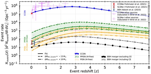
Intrinsic event-rate density, |$\mathcal {R}_{\mathrm{event}}$|, evolution in our fiducial simulations (all solid), the |$\Delta M_{\mathrm{PPI,\, CO\, shift}}= -15 \ \mathrm{M}_{\odot }$| variation (all dashed) and the |$\Delta M_{\mathrm{PPI,\, CO\, shift}}= +10 \ \mathrm{M}_{\odot }$| variation (all dash–dotted). We show our CCSNe transient-event (blue with downward triangle), PPISNe (green with forward slash) and PISNe (orange with vertical line), as well as the BBH-merger rates when we exclude CE systems (solid circles, the line styles match are the same as the transient event-rate variations) and those where we include CE systems (crosses). The translucent green and orange regions indicate the rate ranges spanned by the two variations for PPISNe and PISNe respectively. The other |$\Delta M_{\mathrm{PPI,\, CO\, shift}}$| variations have rates that fall within these regions, except for |$\Delta M_{\mathrm{PPI,\, CO\, shift}}= -20 \ \mathrm{M}_{\odot }$|. We indicate the observed transient event-rate densities of Frohmaier et al. (2021) for CCSNe (red) and SLSNe (pink) as well as the expected GW merger event-rate densities of Abbott et al. (2023) for BBH mergers (blue-gray bar). Moreover, we indicate the event-rate density estimates from other sources for CCSNe and SLSNe, both tabulated in Briel et al. (2022), by pink errorbar symbols and pink capped-errorbar symbols with diamond centers. The (P)PISN-I rates increase in our |$\Delta M_{\mathrm{PPI,\, CO\, shift}}= -15 \ \mathrm{M}_{\odot }$| model and decrease in our |$\Delta M_{\mathrm{PPI,\, CO\, shift}}= +10 \ \mathrm{M}_{\odot }$| model, spanning about an order of magnitude in rate densities for both PPISN-I and PISN-I between the models. CCSNe transient- and BBH-merger rates are not affected in the two models compared to our fiducial model.
In Fig. 4 we also show the volumetric rates at z = 0.028 based on bias-corrected Zwicky Transient Facility (ZTF) observations (Frohmaier et al. 2021). These include the combined hydrogen-rich and hydrogen-poor stripped-envelope CCSNe, at a rate of |$1.151^{+0.15}_{-0.13}\, \times \, 10^{5}\ \mathrm{Gpc}^{-3}\, \mathrm{yr}^{-1}$|, SLSNe-I, at a rate of |$3.5^{+2.5}_{-1.3}\, \times \, 10^{1}\ \mathrm{Gpc}^{-3}\, \mathrm{yr}^{-1}$|. We compare these to our predicted CCSN and (P)PISN-I rates. Moreover, we indicate estimates of CCSNe and SLSNe at higher redshifts from other sources that are tabulated in Briel et al. (2022).
We show the SLSN-I rate because PPISNe-I and PISNe-I may be associated with a subset of SLSNe-I, but we stress that not all PPISNe and PISNe necessarily display SLSNe-like transients. We summarize the SN event-rate results at z = 0.028 from our selected models and compare them to the observations from Frohmaier et al. (2021) in Table 1.
Transient event-rate densities and their ratios to observed rate densities from our fiducial, |$\Delta M_{\mathrm{PPI,\, CO\, shift}}= -15 \ \mathrm{M}_{\odot }$| and |$\Delta M_{\mathrm{PPI,\, CO\, shift}}= +10 \ \mathrm{M}_{\odot }$| models.
| Model | SN type | Rate density|$^{\rm a} \left[\mathrm{Gpc}^{-3}\, \mathrm{yr}^{-1}\right]$| | Ratio to CCSN rate densitya, b | Ratio to SLSN-I rate densitya, b |
|---|---|---|---|---|
| Fiducial | CCSN | |$1.33\, \times \, 10^{5}$| | ||
| PPISN-I | |$1.06\, \times \, 10^{2}$| | |$9.21^{+1.02}_{-1.25}\, \times \, 10^{-4}$| | |$3.03^{+1.12}_{-2.16}$| | |
| PISN-I | |$1.07\, \times \, 10^{1}$| | |$9.30^{+1.03}_{-1.26}\, \times \, 10^{-5}$| | |$0.31^{+0.11}_{-0.22}$| | |
| |$\Delta M_{\mathrm{PPI,\, CO\, shift}}= -15 \ \mathrm{M}_{\odot }$| | CCSN | |$1.33\, \times \, 10^{5}$| | ||
| PPISN-I | |$5.60\, \times \, 10^{2}$| | |$4.87^{+0.54}_{-0.66}\, \times \, 10^{-3}$| | |$16.00^{+5.94}_{-11.43}$| | |
| PISN-I | |$6.05\, \times \, 10^{1}$| | |$5.26^{+0.58}_{-0.71}\, \times \, 10^{-4}$| | |$1.73^{+0.64}_{-1.23}$| | |
| |$\Delta M_{\mathrm{PPI,\, CO\, shift}}= +10 \ \mathrm{M}_{\odot }$| | CCSN | |$1.33\, \times \, 10^{5}$| | ||
| PPISN-I | |$4.10\, \times \, 10^{1}$| | |$3.56^{+0.39}_{-0.48}\, \times \, 10^{-4}$| | |$1.17^{+0.44}_{-0.84}$| | |
| PISN-I | 3.66 | |$3.18^{+0.35}_{-0.44}\, \times \, 10^{-5}$| | |$0.10^{+0.04}_{-0.07}$| |
The ratios to the observed densities for (P)PISNe span about an order of magnitude between our |$\Delta M_{\mathrm{PPI,\, CO\, shift}}= -15 \ \mathrm{M}_{\odot }$| and |$\Delta M_{\mathrm{PPI,\, CO\, shift}}= +10 \ \mathrm{M}_{\odot }$| models. All ratios of PISN-I to CCSN are in tension with Frohmaier et al. (2021), but our |$\Delta M_{\mathrm{PPI,\, CO\, shift}}= -15 \ \mathrm{M}_{\odot }$| model most so.
aAt z = 0.028.
bUsing the observed rate of Frohmaier et al. (2021).
Our fiducial model shows a CCSN transient-rate density of |$\sim {}10^{5}\ \mathrm{Gpc}^{-3}\, \mathrm{yr}^{-1}$| at z = 0, increasing to |$\sim {}7\, \times \, 10^{5}\ \mathrm{Gpc}^{-3}\, \mathrm{yr}^{-1}$| by redshift z ∼ 3 then decreasing to |$\sim {}6\, \times \, 10^{4}\ \mathrm{Gpc}^{-3}\, \mathrm{yr}^{-1}$| at z = 8. Our fiducial CCSN rate, as well as the rates of either variations, match closely the rates of Frohmaier et al. (2021). This indicates that overall we reproduce the observed CCSN-rate density and also that variations in the PPISN mechanism do not affect this rate strongly. This is because the IMF disfavours stars massive enough to undergo PPISN relative to all CCSN progenitors. Overall we find a reasonable match with the other sources for CCSNe that are tabulated in Briel et al. (2022), often matching the lower-bound estimate of the rate.
We find a BBH merger rate of |$\sim {}10\ \mathrm{Gpc}^{-3}\, \mathrm{yr}^{-1}$| at z ∼ 0, excluding systems that undergo CE, which increases to |$\sim {}40\ \mathrm{Gpc}^{-3}\, \mathrm{yr}^{-1}$| at z ∼ 2.5 then decreases to |$\sim {}4\ \mathrm{Gpc}^{-3}\, \mathrm{yr}^{-1}$| at z = 8. These rates are not significantly affected by changes in the CO core-mass range of PPISNe, because the merger rate is dominated by systems with primary masses around |$\sim {}10 \ \mathrm{M}_{\odot }$| (Fig. 2; Li et al. 2021; Veske et al. 2021; Edelman et al. 2022; Tiwari 2022; Abbott et al. 2023). The rate of BBH mergers, if we include those that undergo a CE event and survive, is about a factor of 3 larger than those that exclude CE events over all redshifts. At z = 0.2 the rate including CE systems matches well with GW observations. Section 4.1 shows that our fiducial BBH mergers excluding CE systems match the overall shape of the observed primary-mass distribution well, but here we find that including CE systems is needed to match the observed rate integrated over all BH masses.
Our fiducial PPISN-I transient-rate density at z = 0 is |$\sim {}10^{2}\ \mathrm{Gpc}^{-3}\, \mathrm{yr}^{-1}$|, which increases to |$\sim {}3\, \times \, 10^{3}\ \mathrm{Gpc}^{-3}\, \mathrm{yr}^{-1}$| at z ∼ 3, and then it decreases to |$\sim {}7\, \times \, 10^{2}\ \mathrm{Gpc}^{-3}\, \mathrm{yr}^{-1}$| at z = 8. Our fiducial PISN-I transient-rate density at z = 0 is |$\sim {}10\ \mathrm{Gpc}^{-3}\, \mathrm{yr}^{-1}$|, which increases to |$\sim {}8\, \times \, 10^{2}\ \mathrm{Gpc}^{-3}\, \mathrm{yr}^{-1}$| at z ∼ 3, and then it decreases to |$\sim {}1.5\, \times \, 10^{2}\ \mathrm{Gpc}^{-3}\, \mathrm{yr}^{-1}$| at z = 8. Both our PPISN and PISN rates evolve with redshift but deviate from the shape of the total SFR-density. Both peak at z ∼ 3, coinciding with the cosmic SFR density peak (Fig. D1), but at low redshift (z = 0) their event-rate density is lower, by at least a factor of 5, than at high redshift (z = 8). This is because (P)PISNe occur in very massive stars only, and thus their formation strongly depends on their metallicity. Even if the SFR density at z = 0 (|$\sim 2\, \times \, 10^{7} \ \mathrm{M}_{\odot }\ \mathrm{Gpc}^{-3}\, \mathrm{yr}^{-1}$|) exceeds that at z = 8 (|$\sim 8\, \times \, 10^{6} \ \mathrm{M}_{\odot }\ \mathrm{Gpc}^{-3}\, \mathrm{yr}^{-1}$|), the metallicity distribution at high z trends towards lower metallicities, compensating for their lower SFRs, because stars at lower metallicity lose less mass and remain massive enough to undergo (P)PISN.
In Table 1 we compare our PPISN-I rate density estimate to the inferred SLSN-I rate density of Frohmaier et al. (2021), expressed as the ratio between our predicted and their observed rates. The inferred rate density of SLSNe-I at z = 0.028, |$3.5^{+2.5}_{-1.3}\, \times \, 10^{1}\ \mathrm{Gpc}^{-3}\, \mathrm{yr}^{-1}$|, falls between our predicted PISNe-I and PPISNe-I rates in our fiducial model. With our predicted PPISN-I rate density (at z = 0.028), |$1.06\, \times \, 10^{2}\ \mathrm{Gpc}^{-3}\, \mathrm{yr}^{-1}$|, we find a ratio to the SLSN-I rate of |$3.03^{+1.12}_{-2.16}$| and a ratio to the CCSN rate of |$9.21^{+1.02}_{-1.25}\, \times \, 10^{-4}$|. With our predicted PISNe-I rate density, |$1.07\, \times \, 10^{1}\ \mathrm{Gpc}^{-3}\, \mathrm{yr}^{-1}$|, we find a ratio to SLSNe-I of |$0.31^{+0.11}_{-0.22}$| and a ratio to CCSNe of |$9.30^{+1.03}_{-1.26}\, \times \, 10^{-5}$|. This implies that in our fiducial model (P)PISNe can contribute a significant fraction to the SLSN rate. However, it is important to note that PISNe do not necessarily lead to SLSN-like transients (Gilmer et al. 2017), and the same is likely true in PPISNe (Woosley 2017). We should thus caution making conclusions from directly from these results. Comparison to the other sources that are tabulated in Briel et al. (2022) give similar ratios at higher redshifts.
While shifting the CO core-mass range for PPISNe does not affect the CCSN transient-rate density nor any of the BBH merger rate densities significantly, the PPISN-I and PISN-I rate densities are, however, strongly affected.
With our |$\Delta M_{\mathrm{PPI,\, CO\, shift}}= -15 \ \mathrm{M}_{\odot }$| model both PPISN-I and PISN-I supernova rates increase by about a factor of 5 |$5.60\, \times \, 10^{2}\ \mathrm{Gpc}^{-3}\, \mathrm{yr}^{-1}$| and |$4.10\, \times \, 10^{1}\ \mathrm{Gpc}^{-3}\, \mathrm{yr}^{-1}$|, respectively. This is because, in this model, lower-mass stars explode as PPISNe-I, and because the IMF favours lower mass stars, this rate is higher. With this model both the PPISN-I and PISN-I transient event-rate densities at z = 0.028 are either approximately equal to, or higher than, the inferred SLSN-I rate density. With our predicted PPISN-I rate density we find a ratio to the SLSN-I rate of |$16.00^{+5.94}_{-11.43}$| and a ratio to the CCSN rate of |$4.87^{+0.54}_{-0.66}\, \times \, 10^{-3}$|. With our predicted PISN-I rate density we find a ratio to the SLSN-I rate of |$1.73^{+0.64}_{-1.23}$| and a ratio to the CCSN rate of |$5.26^{+0.58}_{-0.71}\, \times \, 10^{-4}$|. The PISN-I rate density is only slightly higher than the mean SLSN rate and falls within its error bars, but the PPISN-I rate density is higher by more than an order of magnitude.
With |$\Delta M_{\mathrm{PPI,\, CO\, shift}}= +10 \ \mathrm{M}_{\odot }$| both PPISN-I and PISN-I supernova rates are decreased by about a factor of 3 relative to our fiducial model. PPISNe-I decrease to |$4.10\, \times \, 10^{1}\ \mathrm{Gpc}^{-3}\, \mathrm{yr}^{-1}$| and PISNe-I decrease to |$3.66\ \mathrm{Gpc}^{-3}\, \mathrm{yr}^{-1}$|. We now see the effect of the IMF disfavouring increasingly massive stars, decreasing the rate of both phenomena. In this model both the PPISN-I and PISN-I transient event-rate densities are either approximately equal to, or lower than, the inferred SLSN-I rate density. With our predicted PPISN-I rate density we find a ratio to the SLSN-I rate of |$1.17^{+0.44}_{-0.84}$| and a ratio to the CCSN rate of |$3.56^{+0.39}_{-0.48}\, \times \, 10^{-4}$|. With our predicted PISN-I rate density we find a ratio to the SLSN-I rate of |$0.10^{+0.04}_{-0.07}$| and a ratio to the CCSN rate of |$3.18^{+0.35}_{-0.44}\, \times \, 10^{-5}$|. The PPISN-I rate density is approximately equal to the mean inferred SLSN-I rate density, but the PISN-I rate density is lower by more than an order of magnitude.
To summarize, we find that varying the CO core-mass range of (P)PISNe strongly affects the transient event-rate density of these supernovae, with little effect on the overall rates of transients associated with CCSNe. In our fiducial model, both the PPISNe and PISNe could contribute to the SLSN rate. Our |$\Delta M_{\mathrm{PPI,\, CO\, shift}}= -15 \ \mathrm{M}_{\odot }$| model increases both rates such that the rate of PISNe falls within the upper bound of the error on the observed SLSN rate, and the PPISN rate is about a factor of 16-times higher than the mean SLSN rate. Our |$\Delta M_{\mathrm{PPI,\, CO\, shift}}= +10 \ \mathrm{M}_{\odot }$| model has lower (P)PISN transient rates compared to our fiducial model, the PISN rate is about an order of magnitude lower than the SLSN rate and the PPISN rate approximately matches the SLSN rate. We discuss the implications of these variations, and whether they are in tension with the observed SLSN rate, in Section 5.2.
5 DISCUSSION
In the following section we discuss the implications of our results in Section 4, some choices in our modelling approach, and whether, based on our results, the observed peak in the primary-BH mass distribution at |$35 \ \mathrm{M}_{\odot }$| originates from PPISNe.
5.1 PPISN mechanism and the primary-mass distribution
Our modifications to the PPISN prescription of Renzo et al. (2022) encompass both a shift in CO core masses that undergo PPISNe and an additional PPISN or post-PPISN mass loss (equation 6). This parametric approach allows us to explore several physical effects proposed in the literature. We discuss the results of this exploration in this subsection.
Motivated by processes that affect the CO core mass (Section 1) we calculate merging BBH populations with |$\Delta M_{\mathrm{PPI,\, CO\, shift}}= -20 \ \mathrm{M}_{\odot }$| to |$\Delta M_{\mathrm{PPI,\, CO\, shift}}= +10 \ \mathrm{M}_{\odot }$|. Fig. 2 shows that the CO core-mass shift strongly affects the location of the PPISN pile-up in the primary-mass distribution. Moreover, the (relative) magnitude of this pile-up varies with different CO core-mass shifts.
The location and the magnitude of the over-density in our |$\Delta M_{\mathrm{PPI,\, CO\, shift}}= -15 \ \mathrm{M}_{\odot }$| model matches the observed peak at ∼35M⊙. In many of processes mentioned in Section 1, however, this downward shift is too large to explain. The beyond Standard Model process of axion formation, however, could lead to an effective downward shift of as much as |$15 \ \mathrm{M}_{\odot }$| in the model of Mori et al. (2023) where the axion mass is about half the electron mass. They find that supernovae from these axion-induced instabilities are similar to standard pair-formation induced supernovae, i.e. the nickel ejecta distribution has the same overall extent and shape. Their light curves, however, have a shorter rise-to-peak time due to the lower total mass of star, which could differentiate between models, but also means that they do not display the standard long rise-to-peak characteristics used to identify PISNe-I, making it harder to identify them as PISNe-I in SLSN-I observations.
Several of the processes in Section 1 lead to an upward shift of the CO core-mass range of stars that undergo (P)PISNe, but we specifically highlight the more accurate and up-to-date reaction rates and stellar models of Farag et al. (2022), and model this with our |$\Delta M_{\mathrm{PPI,\, CO\, shift}}= +10 \ \mathrm{M}_{\odot }$| model. This model results in an over-density in the primary-BH mass distribution at |$\sim {}64 \ \mathrm{M}_{\odot }$|, suggesting that a third peak in the primary-mass distribution exists. We find that the magnitude of the peak is less pronounced, being only slightly higher (|$0.2\, \times \, 10^{-2}\mathrm{Gpc}^{-3}\, \mathrm{yr}^{-1}\mathrm{M}_{\odot }^{-1}$|) than the merger rate at primary masses slightly lower than the location of the peak (|$58-62 \ \mathrm{M}_{\odot }$|). We expect that the magnitude of this peak relative to the rate at masses slightly lower than the peak, at least in part, depends on the maximum mass of stars that we take into account in our simulations. While our upward CO core-mass shift leads to a larger region of pre-SN core masses that undergo PPISN, if the initial masses of our stars are insufficiently massive to populate the entire range of pre-SN CO core masses, it lowers the rate of BH formation with masses in the expected PPISNe-remnant mass range. In the case that no star is massive enough to undergo PPISN, no pile-up or over-density is formed at all. The range of CO core-masses that undergo PPISN is also a factor that determines the magnitude of the peak. If the range is narrow, fewer stars are in that CO core-mass range, which effectively lowers the rate of stars that undergo PPISN and form BHs in the PPISN-remnant mass range. The narrower CO core-mass range is the result of a higher sensitivity of the PPISN mass loss to the CO core-mass. Examples of this are the σ[12C(α, γ)16O] = −3 models of Farag et al. (2022) or the strongly coupled (high ϵ) hidden-photon models of Croon et al. (2020).
We leave the exploration of the sensitivity of the peak at |$\sim 64 \ \mathrm{M}_{\odot }$| to the maximum considered initial primary mass and the sensitivity of the PPISN mass loss to the CO core-mass for a future study. The O4 observation run of the LVK collaboration (Abbott et al. 2020) probes a five-times larger space than O3 and is expected to uncover more structure in the high mass range. Thus, this peak may already be observed in O4. The exact location and magnitude of this new peak may inform us about the PPISNe mechanism and how massive stars that undergo PPISNe are.
Additionally, we calculate merging BBH populations varying the additional mass loss from |$\Delta M_{\mathrm{PPI,\, extra\, ML}}= +5 \ \mathrm{M}_{\odot }$| to |$\Delta M_{\mathrm{PPI,\, extra\, ML}}= +20 \ \mathrm{M}_{\odot }$|. Fig. 3 shows that additional mass loss lowers the merger rate and moves both |$M_{\mathrm{{PPISN}\, cutoff}}$| and the over-density caused by PPISNe to lower masses, but up to |$\Delta M_{\mathrm{PPI,\, extra\, ML}}= +10 \ \mathrm{M}_{\odot }$|. This is because removing more mass results in primary masses that are created by CCSNe instead of PPISNe, and the BHs that are formed through PPISN lose so much mass that they end up as the secondary BH. The F19 model is similar to our |$\Delta M_{\mathrm{PPI,\, extra\, ML}}= +5 \ \mathrm{M}_{\odot }$| and |$\Delta M_{\mathrm{PPI,\, extra\, ML}}= +10 \ \mathrm{M}_{\odot }$| models, although it does not have the peak in the primary-mass distribution we find at |$\sim {}42 \ \mathrm{M}_{\odot }$| in the |$\Delta M_{\mathrm{PPI,\, extra\, ML}}= +10 \ \mathrm{M}_{\odot }$|. This indicates that a PPISN mass loss prescription that has an artificial discontinuity at the CC-PPISN interface has the same qualitative effect as extra mass removal. While there are studies, both theoretical (Powell et al. 2021; Rahman et al. 2022) and observational (Ben-Ami et al. 2014; Kuncarayakti et al. 2023; Lin et al. 2023), that indicate additional post-PPISN mass loss, removing more than |$10 \ \mathrm{M}_{\odot }$| over the entire range of PPISNe seems hard to justify, and it makes no difference to the primary-BH mass distribution.
5.2 Transient rates
Our fiducial model agrees well with the observed CCSNe rate from Frohmaier et al. (2021). We produce roughly one PISN-I per 10000 CCSNe and one PPISN-I per 1000 CCSNe when z ≤ 1. While currently there are no unambiguous rate estimates from direct observations of PPISNe or PISNe, there are estimates based on the non-detection of these supernovae, e.g. Nicholl et al. (2013). Specifically, from light-curve analysis and SLSN rates, taking into account that not all SLSNe match PISN light curves and that not all PISNe are SLSNe, Nicholl et al. (2013) concludes that the rate of PISNe cannot exceed a fraction |$6\, \times \, 10^{-6}$| of the CCSN rate of. This rate contradicts fiducial results, because we find a ratio of PISNe-I to CCSNe of |$9.30^{+1.03}_{-1.26}\, \times \, 10^{-5}$| (Table 1).
We find that at z = 0.028 our predicted PPISN-I rate is approximately equal to the SLSN-I rate of Frohmaier et al. (2021), and that our PISN-I rate is approximately an order of magnitude lower. We caution, however, that our PPISN-I and PISN-I rates are not directly comparable to observed SLSN-I rates. It is clear from SLSN-I observations (Nicholl et al. 2013; Cia et al. 2018; Gal-Yam 2019) that only a small fraction of SLSNe-I display characteristics that fit with PISNe, and from detailed models of PISNe (Kasen, Woosley & Heger 2011; Nicholl et al. 2013; Gilmer et al. 2017) it is understood that not all PISNe are super luminous or necessarily show the characteristics that make them stand out as PISNe in the SLSNe-I sample. Instead, some PISNe may hide in a population of transients that fall between normal and SLSNe called Luminous Supernovae (Gomez et al. 2022). The situation with PPISNe-I is likely similar. Events like SN2017egm (Lin et al. 2023), iPTF16eh (Lunnan et al. 2018), PTF12dam (Tolstov et al. 2017), and SN 2019szu (Aamer et al. 2023) are strong candidates for SLSNe-I caused by PPISNe-I. However, based on detailed models, not all PPISNe are super-luminous (e.g. Woosley 2017), and the fact that SN 1961V (Woosley & Smith 2022) and iPTF14hls (Wang et al. 2022) possibly have PPISN-like light-curve morphologies but are not super-luminous supports this. Because of the theoretical and observational uncertainties, we refrain here from making quantitative estimates of the fraction of (P)PISNe that appear as super-luminous, and encourage further studies of both PPISN and PISN light curves building on the pioneering work of Woosley (2017), Woosley (2019).
Our fiducial intrinsic transient-rate density predictions at z ∼ 0 for CCSNe and PPISNe-I agree well with the rates of Stevenson et al. (2019; using the compas population-synthesis code). We predict about an order of magnitude more PISNe-I, possibly due to considering a higher maximum stellar mass. The estimates from Briel et al. (2022; using the bpass population-synthesis code) for CCSNe agree well with ours. They estimate a PISN-I rate density of |$1-6\ \mathrm{Gpc}^{-3}\, \mathrm{yr}^{-1}$| at z ∼ 0, which is |$\sim 5\ \mathrm{Gpc}^{-3}\, \mathrm{yr}^{-1}$| lower than our fiducial rate density. They do not provide rate estimates of PPISNe-I. Previous results from Eldridge, Stanway & Tang (2019; bpass) show a similar agreement for CCSNe, and match well for the PISNe-I. Thus, we produce similar CCSNe and PISNe rates to other studies.
We note that with the variations we introduce in this study, specifically our |$\Delta M_{\mathrm{PPI,\, CO\, shift}}$| models, the fractions of (P)PISNe that are SLSNe-I, and vice versa, are not necessarily the same as in our fiducial models. SLSNe from PISNe are characterized by long rise-to-peak times due to large masses, and long decay time-scales. Mori et al. (2023) finds that axion instability supernovae, which we model with a downward CO core-mass shift, behave qualitatively similarly to normal PISNe. The light curves of their PPISNe have a slightly shorter rise-to-peak time, but the nickel-mass ejecta and peak luminosities span the same ranges and are comparable to PISNe without an additional CO core-mass shift. If the light curves and peak luminosities behave similarly, the fraction of PISN-I that are SLSN-I does not change much, and thus, as our fiducial model, our |$\Delta M_{\mathrm{PPI,\, CO\, shift}}= -15 \ \mathrm{M}_{\odot }$| model is likely in tension with the observations. It is unclear how PPISNe, specifically the fraction that display SLSNe-like features, are affected by either an upward or a downward CO core-mass shift, and studies similar to Mori et al. (2023) are necessary to obtain further insight.
To provide a more quantitative exclusion or confirmation of our models, we need observational data from current and upcoming telescopes like JWST (Hummel et al. 2012), LSST (Villar, Nicholl & Berger 2018), EUCLID (Tanikawa et al. 2023), and ROMAN (Moriya, Quimby & Robertson 2022) for better estimates of the rate densities of PPISNe and PISNe, as well as more systematic modelling of PPISNe and PISNe light curves, including variations on stellar evolution and the PPISN mechanism, to determine the fractions of these transients that are super luminous.
5.3 Modelling approach
We use population synthesis to evolve populations with initial primary masses up to |$300 \ \mathrm{M}_{\odot }$| with the binary_c framework. These masses go well beyond the maximum mass of the detailed models on which binary_c is based, and are thus an extrapolation of the fitting formulae from Hurley et al. (2000, 2002), which are themselves based on models of stars with initial masses |$\le 50 \ \mathrm{ M}_\odot$| from Pols et al. (1998). Most of the stars in our simulation that undergo PPISN require initial masses in excess of |$100 \ \mathrm{M}_{\odot }$|, and are affected by systematics in the extrapolation. Our results are affected by the maximum initial primary mass we consider in that the fraction of stars that remain massive enough to undergo PPISN/PISN is changed. The presence of a pile-up in primary BH mass by PPISNe, and probably the magnitude of this pile-up, depend on our considered maximum primary mass. The magnitude of the shallow ‘peak’ of primary BH masses in our |$\Delta M_{\mathrm{PPI,\, CO\, shift}}= +10 \ \mathrm{M}_{\odot }$| model could increase by considering a larger maximum mass. This, in turn, also increases the transient event-rate density of PISNe (Tanikawa et al. 2023).
We choose to use a binary fraction fbin = 0.7. Several studies show that the binary fraction depends on initial primary mass, (e.g. Moe & Stefano 2017; Offner et al. 2022), and in solar-mass stars it is anti-correlated with metallicity (Moe, Kratter & Badenes 2019; Thiele et al. 2023). Because we are interested in objects formed in massive-star systems only, we assume that choosing a mass-dependent binary fraction is currently unnecessary, as most (if not all) massive stars come in binaries or higher-order systems (Sana et al. 2012) or higher multiplicity systems (Offner et al. 2022). Moreover, we assume that the distributions of birth parameters of our binary systems are separable and independent. Moe & Stefano (2017) and Offner et al. (2022) show that this is not the case. Klencki et al. (2018) find, however, that this assumption does not strongly affect the rate estimates, although it does skew the birth mass-ratio distribution of merging BBHs to lower mass ratios.
In this study we use the prescription for PPISN mass loss of Renzo et al. (2022), which is based on the detailed stellar models of F19. Unlike most other existing prescriptions for PPISN mass loss, this provides the mass lost in pulses due to the PPISN, rather than a remnant mass, for a given CO core mass, which allows for a natural transition at the CCSNe/PPISNe boundary. Whether there really is no discontinuity at the interface is unclear (Renzo et al. 2020a), but a prescription that artificially introduces discontinuities should be avoided. Taking the top-down approach from Renzo et al. (2022) makes the final remnant-mass prediction sensitive to the mass of the He layer that lies above the CO core. The pre-SN evolution of the star, specifically the evolution of the mass of the He layer for a given final CO core mass, affects the final remnant mass. Several processes influence the ratio of the He to CO core mass, like convective overshooting (Tanikawa et al. 2021; Vink et al. 2021), or wind mass loss (Renzo et al. 2017; Woosley 2019), or binary interactions (Laplace et al. 2021). We find a near-constant ratio, MHe core/MCO core = 1.3, in all our stars that undergo PPISNe.
5.4 Can the peak in the primary-BH mass distribution at |$35 \ \mathrm{M}_{\odot }$| be explained by PPISNe?
We make use of observations of both GW mergers and EM transient events to constrain our models and to answer whether the peak in the primary-BH mass distribution at |$35 \ \mathrm{M}_{\odot }$| can be explained by PPISNe. We find that the CO core-mass range for stars to undergo PPISNe must shift down by more than |$10 \ \mathrm{M}_{\odot }$| to line up the feature from our PPISNe to the observed feature in the primary-mass distribution at |$35 \ \mathrm{M}_{\odot }$|. This downward shift contradicts recent results (Farag et al. 2022) which suggest an upward shift of about |$10 \ \mathrm{M}_{\odot }$|. Given that the PISNe rate in our fiducial model is already too high according to Nicholl et al. (2013) and that Mori et al. (2023) indicates that the light curves of our |$\Delta M_{\mathrm{PPI,\, CO\, shift}}= -15 \ \mathrm{M}_{\odot }$| model behave similarly to PPISNe without an additional CO core-mass range shift, we find it likely that the downward shift variation that is required to match the GW observations is in tension with the observed (rate of) SLSNe-I.
Our PPISN-prescription variations that behave qualitatively like more recent detailed models of (P)PISNe (|$\Delta M_{\mathrm{PPI,\, CO\, shift}}=+10 \ \mathrm{M}_{\odot }$|) predict a at peak between 58 and 64 M⊙. The transient rates associated with this variation relieve some of the tension with observations, given that only some SLSN-I are PISN-I, although we still overproduce PISN-I compared to Nicholl et al. (2013). Our models therefore suggest that the |$58-64 \ \mathrm{M}_{\odot }$| region is a promising mass range in which to search for a new over-density of primary BH masses, and may well be observable in the next observation runs of the LVK collaboration.
We regard a combination of a downward |$\Delta M_{\mathrm{PPI,\, CO\, shift}}$| variation and |$\Delta M_{\mathrm{PPI,\, extra\, ML}}$| as an unlikely explanation to the peak at |$35 \ \mathrm{M}_{\odot }$|. While additional mass loss does shift the peak to a lower mass, and an additional |$\Delta M_{\mathrm{PPI,\, CO\, shift}}$| of e.g. |$\sim 5 \ \mathrm{M}_{\odot }$| may create an over-density at |$35 \ \mathrm{M}_{\odot }$|, it would still be in tension with the SLSNe rate according to Nicholl et al. (2013) because our fiducial model is already in tension with that rate and any CO core-mass shift would increase this tension.
Current and upcoming transient surveys like EUCLID, JWST, LSST, and ROMAN will measure increased rates of SLSNe, PISNe, and PPISNe over a large range of redshifts. While we cannot definitively rule out downward variation of |$\Delta M_{\mathrm{PPI,\, CO\, shift}}= -15 \ \mathrm{M}_{\odot }$| based on the current observations, these surveys will provide the observational data to confirm or reject our transient-rate estimates, and will statistically constrain the fraction of SLSNe-I is associated with (P)PISNe-I.
Thus, given the results of our study, the fact that transient event-rate observations indicate a likely tension with the rates of our models that lead to a matching peak, we find it unlikely that the observed peak is due to PPISNe.
5.5 If the peak at |$35 \ \mathrm{M}_{\odot }$| is not from PPISNe, then what causes it?
Broadly speaking, the origin of features in the primary-mass distribution are expected to either (i) mainly reflect the remnant mass distribution, or (ii) they mainly reflect (binary) evolutionary selection effects that are caused by their formation channel. If the feature is caused by PPISNe, then this would fall under the first category [e.g. Schneider, Podsiadlowski & Laplace (2023) and Disberg & Nelemans (2023) for the lower-mass analogue]. However, it is equally likely for such a feature to arise from evolutionary effects.
A handful of studies have tried to explain the |$35 \ \mathrm{M}_{\odot }$| peak through causes other than PPISNe and the remnant mass distribution. For example, Antonini et al. (2023) suggests that the |$35 \ \mathrm{M}_{\odot }$| peak can be explained by cluster dynamics. They find that dynamical interactions in globular clusters lead to features in the primary-mass distribution around |$\sim {}35 \ \mathrm{M}_{\odot }$|, as long as massive clusters form with a half-mass density |$\gt 10^{4}\mathrm{M}_{\odot }\, \mathrm{pc}^{-3}$|. This is not populated by hierarchical mergers, but does depend on the dynamical pairing of black holes. Alternatively, Briel et al. (2023) suggests that isolated binary interactions are the cause of the |$35 \ \mathrm{M}_{\odot }$| peak. They find that the peak is not caused by pair-instability remnants, but rather systems that undergo only stable mass transfer, possibly multiple times. They find that a combination of mass-transfer stability that limits the low-end of the mass range of primary-mass BHs at |$35 \ \mathrm{M}_{\odot }$|, and quasi-homogeneous evolution limiting the upper end, leads to an over-density at |$\sim {}35 \ \mathrm{M}_{\odot }$|.
No alternative explanation for the peak at |$35 \ \mathrm{M}_{\odot }$| has yet been adopted as the solution, and further research is needed to determine the correct channel. It may not be enough to just find an over-density at |$35 \ \mathrm{M}_{\odot }$|, and matching other properties of systems around this mass, like mass-ratio (e.g. Li et al. 2022) and spin-orbit alignment, may be critical in finding the actual cause of the observed peak.
6 CONCLUSIONS
We implement a top-down pulsational pair-instability supernova mass-loss algorithm in the binary population-synthesis code binary_c and use this to predict the merger rate and mass distribution of BBHs merging at redshift zero. We explore several physically motivated variations to our PPISN prescription, and study how each variation affects the mass distribution of primary masses of merging BBHs, with a focus on the location of a peak at high BH masses. We combine our GW- and EM-transient predictions to study PPISNe and PISNe phenomena, and we compare these to recent observations to constrain our model variations.
Below we list our most notable results.
Our fiducial model has no peak in the primary-mass distribution that matches the observed feature at |$35 \ \mathrm{M}_{\odot }$|.
Our CO core-mass shift variations strongly affect the location of the PPISN pile-up such that shifting the CO core-mass range with |$\Delta M_{\mathrm{PPI,\, CO\, shift}}= -15 \ \mathrm{M}_{\odot }$| does match the location of the observed over-density in the primary-mass distribution. It is hard to explain this with conventional physics like rotation or variations in nuclear reaction rates. The upward shift of |$\Delta M_{\mathrm{PPI,\, CO\, shift}}= +10 \ \mathrm{M}_{\odot }$|, which is based on detailed models of PPISNe (Farag et al. 2022), moves the over-density upward in primary BH mass by about |$8-14 \ \mathrm{M}_{\odot }$|, predicting a (slight) over-density at |$58-64 \ \mathrm{M}_{\odot }$|. The current LVK O4 observation run will detect BBH systems more efficiently than before and could shed light on whether this third peak exists.
Our additional mass-loss variations affect the location of the over-density of BHs in the primary-mass distribution by about |$5-10 \ \mathrm{M}_{\odot }$|. Removing more mass, however, does not lead to an over-density at lower masses because, at lower mass, the majority of BHs with those primary-masses are created through CCSNe.
The transient-rate estimates of CCSN in our fiducial model match well with the inferred rate of Frohmaier et al. (2021). Their rate for SLSN-I falls between both our predicted PPISN-I and PISN-I rates. We predict a PPISN rate ∼3-times higher, and a PISN rate ∼3-times lower. Our ratio of PISN-I to CCSN-I exceeds the estimate of Nicholl et al. (2013), however, indicating that our fiducial model disagrees with the SLSN-I rate.
With the PPISN-prescription variation that does produce a peak at the correct location (|$\Delta M_{\mathrm{PPI,\, CO\, shift}}= -15 \ \mathrm{M}_{\odot }$|), we find that the PPISN-I rates exceed the SLSN rates by a factor of 16, and the PISN-I rates are almost double that of the SLSN-I rates. Even taking into account that not all (P)PISNe produce SLSNe, and not all SLSNe can be explained by (P)PISNe, these rates likely are in tension with the observed SLSN rates as well.
In summary, because the large downward shift in CO core mass required to fit the observed GW peak is difficult to explain without exotic physics beyond the Standard Model, and new reaction rate studies even suggest an upward shift to |$58-64 \ \mathrm{M}_{\odot }$|, and because the transient event-rates of PPISNe and PISNe for this variation are likely in tension with the observed SLSNe rate, we conclude that PPISNe are unlikely to be responsible for the peak feature observed at |$32 -38 \ \mathrm{M}_{\odot }$|.
Acknowledgement
DDH wants to thank Arman Aryaeipour, Max Briel, Payel Das, Will Farr, Giovanni Mirouh, Bob Nichol, Natalie Rees, Karel Temmink, and Rob Yates for the useful discussions, Paula Gherghinescu and Madison Walder for their artistic advice, and the UKRI/UoS for the funding grant H120341A. LvS acknowledges partial financial support from the National Science Foundation under Grant No. (NSF grant number 2009131), the Netherlands Organisation for Scientific Research (NWO) as part of the Vidi research program BinWaves with project number 639.042.728 and the European Union’s Horizon 2020 research and innovation program from the European Research Council (ERC, Grant agreement No. 715063). RGI thanks the STFC for the funding grants ST/R000603/1 and ST/L003910/2, and the BRIDGCE consortium. The authors thank Selma de Mink for providing a platform for collaboration and communication, and for long term scientific guidance. Moreover, we thank the anonymous reviewer for the useful feedback on the manuscript.
In this research we make use of the GWTC-3 data release provided by the LIGO, VIRGO, and KAGRA collaborations (LIGO Scientific Collaboration, Virgo Collaboration & KAGRA Collaboration 2021). Moreover, we make use of the following software to enable this study: The cosmology module of astropy (The Astropy Collaboration 2022), asymmetric_uncertainty (Gobat 2022), the SFR prescriptions of compas (Riley et al. 2022) h5py (Collette 2013), ipython/jupyter (Perez & Granger 2007; Kluyver et al. 2016), matplotlib (Hunter 2007), numpy (Harris et al. 2020), numpy-indexed (Hoogendoorn 2023), pandas (Wes McKinney 2010; The pandas development team 2020), pycbc (Nitz et al. 2023), PyPDF2 (Fenniak et al. 2022), pytables (PyTables Developers Team 2002), python (Van Rossum & Drake 2009), and scipy (Virtanen et al. 2020).
DATA AVAILABILITY
We make the DCO and EM transient data used in this study available on 10.5281/zenodo.8083112 upon publication, along with routines to generate these data and the figures presented in this paper. The data is generated with a modified version of binary_c v2.2.2 and a modified version of binary_c-python v0.9.5/2.2.2.
References
APPENDIX A: REMNANT MASSES OF SINGLE STARS
In Fig. A1 we show how our fiducial prescription for PPISN mass loss, the F19 model for PPISNe mass loss, and examples of our two variations affect the remnant-mass prediction as a function of initial stellar (ZAMS) mass and metallicity. The final mass is determined by a combination of wind mass loss, compact-object formation by CCSNe, black hole formation by PPISNe, and total disruption by PISNe.
In Fig. A1(a) we show the fiducial remnant masses as a function of initial mass and metallicity, in Fig. A1(b) we show the remnant masses as predicted with the F19 variation, in Fig. A1(c) we show an example of variation with an extra mass loss of |$\Delta M_{\mathrm{PPI,\, extra\, ML}}= 10 \ \mathrm{M}_{\odot }$|, and in the Fig. A1(d) we show the final mass predictions for the CO core-mass shift variation of |$\Delta M_{\mathrm{PPI,\, CO\, shift}}= -5 \ \mathrm{M}_{\odot }$|.
In the F19 variation, Fig. A1(b), we see that the region of ZAMS masses that undergo PPISNe is not strongly affected, but the supernova type that leads to the most massive BH is now a CCSN. Moreover, the remnant masses Fig. A1(c) match well with those in Fig. A1(b), which indicates that in binary_c the F19 prescription results in a discontinuity between the last CCSN and the first PPISN of about |$10 \ \mathrm{M}_{\odot }$|.
In the CO core-mass shift variation, Fig. A1(d), the ZAMS mass and metallicity region is shifted to lower mass and higher metallicity compared to our fiducial model, Fig. A1(a), with for the lowest metallicity, a downward shift of the ZAMS mass for the PPISNe region by about |$10 \ \mathrm{M}_{\odot }$|. The lower ZAMS-mass requirement leads to an increase in the highest metallicity for which the PPISNe occur, in this case from |$3\, \times \, 10^{-3}$| to |$5\, \times \, 10^{-3}$|.
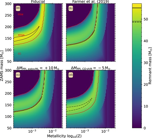
Remnant-mass distribution in our single star grid as a function of ZAMS masses (abscissa) and metallicities (ordinate). The colour-scale indicates the final remnant mass. The four panels show our fiducial PPISN model (a), the F19 model (b), and two examples of our variation on the PPISN prescription, the first being the extra mass loss variation (c) and the second the core-mass shift variation (d). The thin red line indicates the region of ZAMS mass and metallicity where the single star undergoes PPISN + CC. The region in the top left corner is where stars undergo PISN and leave no remnant. The remaining region indicates stars that undergo CC only. The black lines of various line styles indicate regions with remnant masses within |$1 \ \mathrm{M}_{\odot }$| of the maximum mass in each distribution. For the models F19 and |$\Delta M_{\mathrm{PPI,\, extra\, ML}}= +10 \ \mathrm{M}_{\odot }$| these regions overlap and we indicate them with the same line style.
APPENDIX B: FIDUCIAL PRIMARY-MASS DISTRIBUTION INCLUDING SYSTEMS THAT UNDERGO AND SURVIVE CE
In this study we calculate the properties of merging BBH systems from simulations with varying assumptions on the remnant mass predictions from PPISNe, and compare them to observed distributions. In the results in Sections 4.1 and 4.2 we exclude systems that undergo one or more CE episodes. Here we show which mass ranges are most affected by this.
In Fig. B1 we show a comparison between our fiducial model where CE systems are excluded and those where CE systems are included. Below |$14 \ \mathrm{M}_{\odot }$| systems that undergo and survive CE systems contribute significantly to the total merger rate (>40 per cent), especially around the peak at |$10 \ \mathrm{M}_{\odot }$|. Between |$14 \ \mathrm{M}_{\odot }$| and |$25 \ \mathrm{M}_{\odot }$| BBH mergers that undergo and survive CE contribute, but not as much as the other channels (<40 per cent).
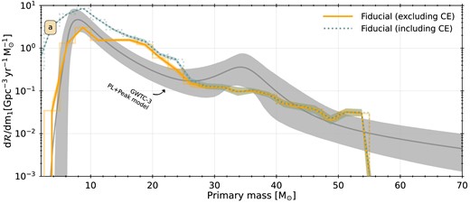
Panel (a): Distribution of primary masses for BBH systems merging at z = 0.2. The dark grey line indicates the mean of the power law + peak model z = 0.2 and the grey shaded region indicates the 90 per cent confidence interval. The orange line and region shows the mean and 90 per cent confidence interval of our fiducial model results that exclude CE systems. The blue dotted line and region shows the mean and 90 per cent confidence interval of our fiducial model results that include CE results.
APPENDIX C: SUPERNOVA-KICK SCALING
In this study we sample the BH kick speed from a Maxwellian velocity distribution (Hobbs et al. 2005) and we scale this kick by (1 − ffallback), which measures how much of the initially ejected mass actually is lost from the system (Section 2.1.5). There is, however, some debate on whether BHs do receive kicks and of what amplitude (e.g. Dray et al. 2005; Renzo et al. 2019; Atri et al. 2019; Callister, Farr & Renzo 2021)
Because the velocity distribution of supernova kicks of Hobbs et al. (2005) is based on observed pulsars, i.e. neutron stars, a different scaling approach is based on that the kick distribution should be regarded as a momentum kick distribution, and that the velocity kicks for BHs should be scaled by the ratio of the BH remnant mass to the neutron star mass (taken as |$1.4 \ \mathrm{M}_{\odot }$|) to conserve momentum as
where MNS is the NS mass and Mremnant is the remnant BH mass.
There are indications that BH kick speeds are indeed lower than those for NSs (e.g. Mandel 2016; Atri et al. 2019). There are, however, also studies that show that black holes can still attain high-velocity kicks, based on theory and simulations (e.g. Janka 2013; Chan, Müller & Heger 2020) motivated by strong asymmetries in the ejecta and the ’tug-boat’ mechanism.
Moreover, there does not seem to be a consensus in the population-synthesis studies on which scaling should be used. For example van Son et al. (2022a) uses fallback-only scaling, while Briel et al. (2023) only scales by the NS-mass to remnant-mass ratio. Giacobbo & Mapelli (2020) compares different (combinations of) scaling factors and finds that these different prescriptions do not affect the BBH-merger rate significantly.
For the mass range in primary BH mass MBH, 1 relevant here, the merging BBH systems in our fiducial models achieve to merge thanks to the eccentricity induced by the kick onto the lower mass companion. We calculate the ratio between the (MNS/Mremnant) scaling factor and the (1 − ffallback) scaling factor to estimate the how this would affect our results. The colour in Fig. C1 shows the merger rate of BBH systems in our fiducials models as a function of primary mass and the ratio of kick-scaling factors of secondary BHs in systems where the secondary BH recieves a kick. The plot shows that for the majority of mergers the ratio is below 1, indicating that the (1 − ffallback) scaling factor is larger than with the (MNS/Mremnant) scaling. Thus, for the majority of mergers that recieve a kick, the kick is lower than what it would be with the (MNS/Mremnant) scaling. Over the entire range we do find a spread in the ratio of the two scaling factors, mostly between 0.2 and 4, except for some systems with primary BH masses around |$15 \ \mathrm{M}_{\odot }$|, indicating that in those systems the secondary BH kick would be scaled down more. Using the (MNS/Mremnant) scaling leads to higher kicks (so presumably higher post-CC eccentricities, but also higher disruption rates) at the formation of the secondary BH for the majority of the merging systems. A combination of both scalings may be appropriate (Giacobbo & Mapelli 2020), but our fallback scaling already leads to a dampening of many of the kicks comparable to what the (MNS/Mremnant) scaling would do.
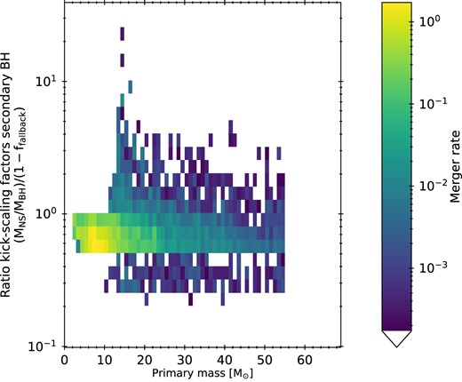
Merger rate of BBH systems in our fiducials models as a function of primary mass (ordinate) and the ratio of kick-scaling factors of secondary BHs (abcissa). Overall, the fallback scaling factors are larger than the (MNS/Mremnant) for most of the merging BBH systems. Around |$M_{\mathrm{primary}}\, \sim 15 \ \mathrm{M}_{\odot }$| there are secondary BHs that would get significantly lower kicks, but this is only the case for a few systems.
APPENDIX D: MERGER-RATE CALCULATION
In our population-synthesis framework binary_c we take a grid-based approach to sample the properties of the systems in our populations. We use the distributions of the birth properties primary mass (M1), secondary mass (M2), period (P) (Section 2.2) to span a hypercube which we split up into equally sized volumes of phase-space. Each of these volumes represents a system with a set of birth properties, ζi, and a probability pi. We use this probability to calculate the number of systems this system represents (Ni) in a population of Nbin binaries. We combine this probability with the binary fraction, fbin, to take into account the fact that not all systems are binary systems, which allows us to calculate Ni given a population of single and binary systems Nsystems,
In this study we are, however, more interested in the rate of formation and merging of systems than in their total number. To calculate the rate of formation of system i, Ri, we combine equation (D1) with a SFR and the average mass of a system,
where |$\frac{\mathrm{SFR}}{\left\langle M\right\rangle }$| is the rate of formation of all systems and <M > is the average mass of all systems, <M >. We calculate this average mass by integrating the mass distributions between their global bounds, in both single and binary systems (see Section 2.2) and obtain an average system mass of |$\left\langle M\right\rangle = 0.689 \ \mathrm{M}_{\odot }$|.
To calculate the merger-rate density, |$R_{\mathrm{merge},\, i}$|, of a system with a metallicity, Zi, and a delay time, |$t_{\mathrm{delay},\, i}$|, at a given merger redshift, zmerge, we modify equation (D2) to calculate the SFR density at the birth redshift, zbirth, of system, i, given that the system merges at redshift zmerge,
where Zi is the metallicity of the system and dZi is the width of the metallicity bin in which the system lies. |$z_{\mathrm{birth},\, i}$| corresponds to the birth-redshift of the system, which is determined by calculating the birth lookback time |$t^{*}_{\mathrm{birth},\, i} = t^{*}_{\mathrm{merge}} + t_{\mathrm{delay},\, i}$| and converting it to the corresponding redshift using the cosmology defined in Section 2.3. We repeat this for all systems at all metallicities.
Fig. D1 shows the SFR distribution, along with the extent of the metallicities we use, in our input populations and the individual metallicities.
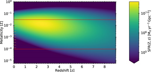
SFR density, SFR(z, Z) used to convolve our BBH systems (van Son et al. 2022a), as a function of redshift (ordinate) and metallicity (abscissa). The colour indicates the SFR density, the red lines indicate the extent of our metallicity grid, and the orange dashed ticks on the left are the metallicities of the binary populations we simulate.
