


ABSTRACT
We construct simple models to explore in principle whether the backwarming by radiation from infalling envelopes can significantly heat and change the structure of protoplanetary discs. The motivation for this investigation is the recent study of a small subset of Orion protostars by Karnath et al., who argued that the bright, extended, and irregular sub-mm and mm emission did not arise from protostellar discs because the images were not elongated as expected. We therefore constructed simple disc models to see whether heating from the envelope surrounding a disc could in principle significantly increase disc scale heights and thus produce less-elongated images. We assume steady accretion and solve the radiative transfer self-consistently. For central luminosities and envelopes roughly comparable to the Karnath et al. protostars, we find that while envelope irradiation can significantly heat the discs, the magnitude of the effect only increases scale heights by modest factors, and so our models cannot easily account for the observed morphologies. We speculate that dynamical perturbations by companion protostars might be responsible for the observed complex structure.
1 INTRODUCTION
Infrared and far-infrared surveys with the Spitzer Space Telescope and the Herschel Space Telescope have had a major impact on our understanding of protostellar populations (e.g. Evans et al. 2009; Megeath et al. 2012; Stutz et al. 2013; Dunham et al. 2014; Furlan et al. 2016; Fischer et al. 2017). In addition, improvements in mm-wave capabilities have led to much better characterization of disc properties in these protostellar samples (Maury et al. 2019; Tobin et al. 2020). The sensitivity and scope of these surveys have enabled the characterization of statistically significant samples of protostars, helping to develop a better picture of protostellar disc evolution (see e.g. the extensive overview presented in the introduction of Tobin et al. 2020). In particular, the large samples now available make it possible to identify rare objects in short-lived evolutionary stages, such as those represented by the Class 0 objects (Andre, Ward-Thompson & Barsony 1993).
A major goal of protostar studies is the detection and analysis of the youngest protostars to test theories of star formation. It is plausible that the youngest protostars might be the most heavily extincted by their dusty envelopes, given that infall rates might be highest early on (Foster & Chevalier 1993; Henriksen, Andre & Bontemps 1997); in addition, the angular momenta of the first material to fall in may be lowest, resulting in infall closer to the central protostar (Cassen & Moosman 1981; Terebey, Shu & Cassen 1984) and larger extinctions for a given infall rate (e.g. Kenyon, Calvet & Hartmann 1993). In this regard, the ‘PACS bright red sources’ (PBRs) in Orion, identified by Stutz et al. (2013) as having extremely red 70–24 µm flux ratios, are of special interest as likely very young systems. Further evidence in support of their youth is provided by the large masses in their near environments (0.2–2 M⊙; Stutz et al. 2013).
As part of the VLA/ALMA Nascent Disk and Multiplicity (VANDAM) survey of Orion protostars (Tobin et al. 2020), a subset of PBRs were shown to be especially bright at 0.87 and 8 mm as imaged with Atacama Large Millimeter and Submillimeter Array (ALMA) and with the Very Large Array (VLA), respectively. Six of these objects were studied extensively by Karnath et al. (2020, hereafter K20) because of their special properties, with three of these objects showing very extended (≳100 au), irregular structures atypical of the VANDAM sample (Sheehan et al. 2022; see also Maury et al. 2019). In their appendix, K20 note some structural properties of their sources. HOPS 400B has a bright central peak that is offset from the geometric centre of the mm emission extending over 200 au in diameter; HOPS 402 has a triangular structure at 8 mm; HOPS 403 has roughly circular symmetry over a 150 au diameter region, with an elongated peak to the south-east; and HOPS 404 has a box-shaped morphology at 8 mm.
Importantly, K20 inferred that HOPS 400B, 401, 402, 403, and 404 (hereinafter HOPS 40x) were optically thick at the shortest wavelengths based on the 0.87 mm/8 mm flux ratios. Using the 0.87 mm imaging to set the brightness temperature, and with a guess at the 8 mm opacity, K20 derived remarkably large (gas) masses of ∼0.2–2 M⊙ for these objects and radii as large as 80 au. These are very much larger than typical values from the VANDAM survey, ∼2 × 10⁻³ M⊙ (assuming a gas-to-dust ratio of 100) and ∼30 au (Sheehan et al. 2022).
So what are these dusty structures? The most straightforward explanation of these structures is that they are dusty, massive protostellar discs. Disc formation is a natural outcome of the collapse of protostellar clouds with finite angular momentum; discs are commonly found around protostars; and the VANDAM survey found a typical protostellar dust disc radius of ∼45 au (Tobin et al. 2020), comparable to the HOPS 40x sources.
However, K20 did not favour the disc interpretation because the images did not show the expected flat structure. To support their argument, K20 argued that the outflows of HOPS 403 and 404, which are extended in the plane of the sky, would suggest an edge-on disc orientation assuming that the outflows are oriented in the perpendicular direction, and thus the mm dust emission should be clearly elongated. They instead conjectured that these objects are collapsing protostellar fragments.
In this paper, we use simple models to explore whether a protostellar disc backwarmed by radiation from its envelope might be less flattened intrinsically than intuitively expected. The reason is that the envelope intercepts far more radiation from central regions than a flat or even modestly flared disc, and the resulting re-emission can produce significant heating of the disc (Butner et al. 1991; Butner, Natta & Evans 1994; D’Alessio, Calvet & Hartmann 1997). This extra heating will result in an increase in the disc scale height and thus a thicker disc, which will appear less flattened. In addition, the increase in disc thickness may make it less favourable for detection at high inclination angles because of disc extinction of central regions (e.g. D’Alessio et al. 2006). Envelope backwarming can also be important in explaining the very bright mm-wave emission of these objects.
Our models are not intended to fit the HOPS sources, as the former are simple and axisymmetric (to illustrate the basic physics), while the latter are not. We do, however, explore a parameter space comparable to the HOPS objects, as the high mm-wave fluxes of these objects and their inferred high envelope infall rates suggest that backwarming effects might be higher than typical of protostars.
The irregular structure seen in the ALMA and VLA images ultimately will require complex dynamical models for best comparisons. However, there is value in constructing axisymmetric, simple disc and envelope models, as we present in this paper, that have a minimum of parameters as a starting point for further exploration.
2 MODELS AND METHODS
To calculate the structure of the disc irradiated by the external envelope, we use the D’Alessio irradiated accretion disc (DIAD; D’Alessio et al. 2006) models, expanded to calculate separately the dust and gas temperatures (Espaillat et al. 2022), and modified to include irradiation by a surrounding envelope, following D’Alessio et al. (1997). Here, we provide an overview of the calculations. We assume that the disc is in hydrostatic equilibrium and it is heated by radiation originating in the photosphere, accretion shock, and corona, transported through the envelope and arriving in the disc from all directions. The disc is assumed to accrete steadily at a rate |$\dot{M}$|, with transport modelled by the α viscosity. While viscous dissipation is included in the energy equation, at the radii of interest here, the disc is heated mainly by the external radiation fields. Dust settling and heating are treated as in D’Alessio et al. (2006), with the flux from the envelope crossing the equatorial plane used as the external boundary condition for the disc. The equations of conservation of energy and hydrostatic equilibrium are solved to get the vertical structure and each radius. Since the high-energy radiation fields that heat the gas are severely attenuated by the envelope, gas and dust temperatures are essentially kept the same by collisions between the two phases. The vertical structure is iterated until the surface density at the mid-plane is equal to the viscous surface density for given |$\dot{M}$| and α such that hydrostatic equilibrium is maintained.
The infalling envelope is modelled using the Ulrich (1976) and Terebey et al. (1984) density structure with the temperature structure calculated as in Kenyon et al. (1993). While the impact of the envelope on the disc could create significant perturbations and shear, producing dust substructures (Kuznetsova et al. 2022), we ignore such effects in this simple model.
The flux from the envelope arriving at each radius of the disc is calculated by integrating the specific intensity arriving at the given radius over solid angle and frequency. In turn, the specific intensity is calculated by solving the transfer equation at each frequency along rays centred on the radius covering the hemisphere above the equatorial plane. This flux is used as boundary condition for the solution of the disc vertical structure. The transition between the disc and the envelope is taken to be at the height where the disc thermal pressure is matched by the total envelope pressure |$P(\textrm {thermal}) = \rho _{\textrm {in}} v_{\theta }^2$|, where ρin is the density of the envelope and the velocity is the θ-component of the velocity field in spherical coordinates, a simple approximation to the vertical velocity to the flared disc ‘surface’. For the parameters adopted here, the transition between envelope and disc occurs at several scale heights above the mid-plane, justifying our neglect of dynamical effects of infall on disc structure.
The envelope structure is parametrized by a scaling density ρ1 and a centrifugal radius Rc (see Terebey et al. 1984; Kenyon et al. 1993). The density parameter is related to the mass infall rate by |$\dot{M}_{\textrm {in}} = 4 \pi \rho _1 (1 \textrm {au})^{3/2} (2 G M_*)^{1/2}$|, and is useful because the stellar mass M* is generally not known and infall velocities i(2GM*/r)1/2 are not well determined or unobserved. Among the disc parameters are the (steady) mass accretion rate of the disc, |$\dot{M}_\mathrm{ d}$|, the viscosity parameter, α, the dust settling parameter, ϵ, which gives the dust depletion relative to the standard interstellar medium dust-to-gas mass radius (D’Alessio et al. 2006). Other parameters are the stellar mass M*, radius R*, and luminosity L*, along with the accretion luminosity |$L_{\textrm {acc}} = G \dot{M}M_*/R_*$|.
For both the envelope and the disc, we assume dust size distributions proportional to a−3.5, between a minimum size amin = 0.005 µm and a maximum size amax used as a parameter. For the envelope, we adopted amax = 0.25 µm, while the amax = 0.1 mm opacity was adopted for the disc (see Fig. 1). The dust consists of silicates and graphite, with abundances in the envelope following D’Alessio et al. (1997) and in the disc following D’Alessio et al. (2006). Note that we did not assume any settling of the disc dust in order to maximize the possible thickness of the disc seen in emission.
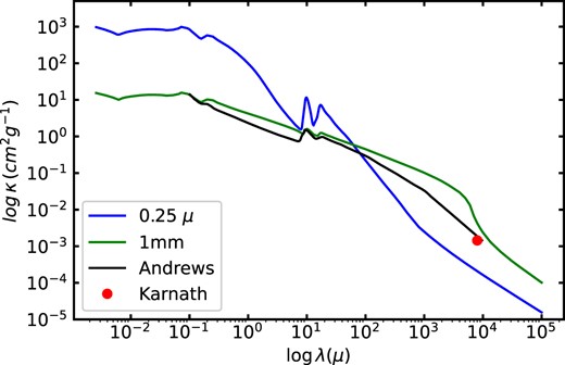
Dust opacities used in the calculations. These assume a dust-to-gas mass ratio of 100 to correspond with gas masses. The amax = 0.25 µm opacity was used for the envelopes, while the amax = 0.1 mm opacity was adopted for the discs. The black curve shows a comparable disc dust opacity from Andrews et al. (2009) and the red dot shows the 8 mm opacity adopted by K20.
We used RADMC3D (Dullemond et al. 2012)1 to compute the images. The DIAD models are calculated on a cylindrical grid; they were mapped to spherical coordinates for use in constructing images and Spectral Energy Distributions (SEDs) for models that include both the disc and its envelope. While RADMC3D can also be used to compute the temperature distribution of a given density structure, the methods described above allow for enforcement of the vertical hydrostatic equilibrium and for adjustment of the surface density distribution for a given α viscosity and mass accretion rate. We have checked the RADMC3D temperature distribution assuming the structure given by the D’Alessio et al. (1997) methods and find reasonably good agreement, especially considering that our models include viscous heating of the disc.
3 RESULTS
For Models 1–5, we assume a central protostellar mass, luminosity, and radius of M* = 0.5 M⊙, L* = 1 L⊙, and R* = 2 R⊙. For Model 5, we assume M* = 1 M⊙, L* = 3.5 L⊙, and R* = 2.5 R⊙. The accretion luminosity is |$L_{\textrm {acc}} = G M_* \dot{M}/R_*$|, and is added to the stellar luminosity to provide the total L = L* + Lacc that irradiates the disc and envelope. The range of luminosities studied has been chosen to correspond to the ∼0.6–5 L⊙ span of the HOPS 40x sources (K20). The outer radii of the discs are all set to 100 au, which is at the upper end of the deconvolved radii found by K20.
The envelope parameters are loosely based on the spectral energy distribution fitting of the HOPS 40x sources by Furlan et al. (2016). Scaling their values of ρ at 1000 au to our parameter yields |$\rho _1 \sim 2\!-\!8 \times 10^{-13}\, {\rm g \, cm^{-3}}$|. The values of the centrifugal radii are relatively large, Rc ∼ 50–500 au, particularly in view of the image sizes indicated by the mm observations. We therefore adopt smaller values of Rc more comparable to the implied disc sizes, and |$\rho _1 = 1\!-\!3 \times 10^{-13} \,{\rm g \, cm^{-3}}$|, as the SED modelling generally shows a trade-off between the centrifugal radius and the reference density |$\rho _1 \approx R_\mathrm{ c}^{1/2}$|. We note that for a central mass of 0.5 M⊙, the lower value of ρ1 corresponds to a mass infall rate |$\dot{M}_{\textrm {in}} = 1.3 \times 10^{-5}\, {\rm M}_{\odot }\, {\rm yr^{-1}}$|. This is much larger than the assumed accretion rates through the disc, based on limits on the total luminosity, so would imply substantial piling up of disc mass over time (e.g. Kenyon et al. 1990). The parameters for both discs and envelopes are summarized in Table 1.
Model parameters.
| Model | La | |$\dot{M}$|b | α | |$M_{\mathrm d}$|c | |$\rho _1$|d | |$R_{\mathrm c}$|e | Qf |
|---|---|---|---|---|---|---|---|
| 1 | 1.77 | 1 × 10⁻⁷ | 0.01 | 0.046 | 1 × 10⁻¹³ | 10 | 2.42 |
| 2 | 2.54 | 2 × 10⁻⁷ | 0.01 | 0.097 | 3 × 10⁻¹³ | 10 | 1.75 |
| 3 | 1.77 | 1 × 10⁻⁷ | 0.0033 | 0.16 | 3 × 10⁻¹³ | 10 | 0.97 |
| 4 | 1.77 | 1 × 10⁻⁷ | 0.0033 | 0.16 | 3 × 10⁻¹³ | 50 | 1.06 |
| 5 | 3.52 | 1 × 10⁻⁷ | 0.0033 | 0.17 | 3 × 10⁻¹³ | 50 | 1.19 |
Luminosity in L⊙.
Accretion rate in |${\mathrm{ M}_{\odot}}\,\mathrm{ yr}^{ -1}$|.
Disc gas mass in M⊙.
Envelope scaling density in g cm−3 (see text).
Centrifugal radius in au.
Toomre parameter Q measured at 75 au.
We have also computed disc models with no envelope for comparison purposes. These models have the same central luminosity, accretion rate, and α parameter, and assume in all cases the same outer disc radius of 100 au.
3.1 Model properties
Fig. 2 shows the density distributions of Model 4 at two spherical radii as a function of polar angle θ. This illustrates how the envelope has been joined to the disc. For comparison, we also show the corresponding density distributions of a disc model with the same central luminosity, accretion rate, and viscosity parameter, but without an envelope. (The structure has been truncated at low densities to avoid numerical instabilities in the original model.)
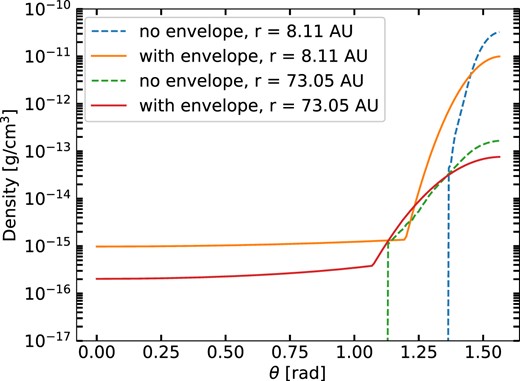
Gas density versus θ, the angle measured from the disc vertical axis, at two selected spherical radii. One set of curves is for Model 4 with envelope, the other for the corresponding disc model without an envelope.
To understand the differences in density structures, in Fig. 3 we show the corresponding temperature distributions at the same radii. The envelope backwarmed discs are essentially vertically isothermal2; this results in nearly Gaussian vertical density distributions. In contrast, the disc models without envelopes show the usual heating of the upper layers of the disc, with the cooler mid-plane (except at small radii, where viscous heating becomes important in the central disc regions; D’Alessio, Calvet & Hartmann 2001).
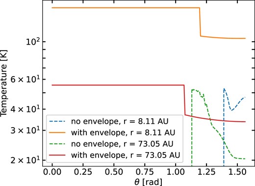
Gas temperature versus θ, at two selected spherical radii for Model 4 with envelope, and for the corresponding disc model without an envelope.
The density scale heights at small radii are much larger than that of the no-envelope disc because the temperatures are much higher; at large radii, the effect is smaller because the temperatures are more similar.
3.2 Parameter dependence
We find that the disc temperatures follow T ∼ (L/4πσR2)1/4 fairly closely (Fig. 4). At the smallest radii, the disc temperatures are higher because of radiative trapping in the envelope. At larger radii, the disc temperatures fall off somewhat faster than R−1/2 but then show a maximum near rc, as also found by D’Alessio et al. (1997). This is due to the pileup of density near the centrifugal radius in the Ulrich (1976) and Cassen & Moosman (1981) infall model, which helps trap radiation. Overall, the disc temperatures are relatively weakly dependent upon the central luminosity as T ∝ L1/4.
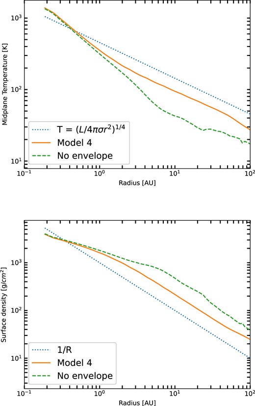
Upper panel: Mid-plane temperature T(R) for Model 4, with and without envelope. The temperature distributions are slightly below T4 = L/4πσR2, with a slightly steeper falloff with R in general. The exception is at small radii, where the disc temperature is elevated by internal viscous dissipation. There is a slight bump at R ∼ rc due to the pileup in density of the envelope model (see text). Bottom panel: Σ(R) for the same models as in the upper panel. The surface density shows the roughly 1/R dependence expected for a constant accretion rate viscous disc with T ∝ R−1/2, with variations anticorrelated with T(R) departures from the power law.
With the assumption of a constant accretion rate and α, a temperature structure T ∼ R−1/2 leads to Σ ∼ R−1 (Hartmann et al. 1998). Fig. 4 shows that the surface density falls off a bit less steeply with increasing radius because of the slightly steeper dependence of T on R.
Fig. 5 shows the mid-plane temperature distributions of the other models. In general, the run of T(R) is quite similar, suggesting that T(R) ∼ f(L/4πR2)0.25 is adequate for a rough estimate, with f ∼ 0.6–0.7. The small bump in the temperature distribution occurs near 10 au for models 1, 2, and 3, and near 50 au for model 5, consistent with their centrifugal radii (Table 1). Model 1 has the lowest temperatures, as expected because of its lower luminosity and lower envelope density, the latter resulting in less backwarming of the disc.
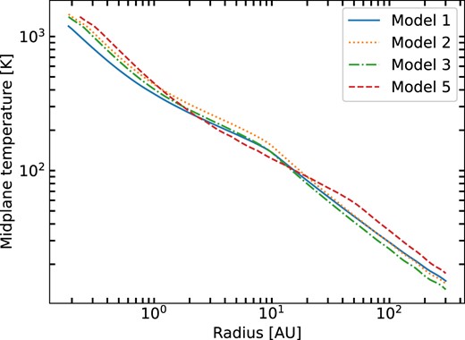
Model mid-plane temperature distributions for models 1, 2, 3, and 5.
Fig. 6 shows the corresponding surface densities of the models shown in Fig. 5. In the steady disc model, |$\Sigma \propto \dot{M}\ (\alpha c_{\mathrm s} H)^{-1} \propto \dot{M}\Omega (\alpha T)^{-1}$|, where H is the scale height, cs the sound speed, and Ω the Keplerian angular velocity. For a fixed outer disc radius, one would then expect the disc mass to scale as |$\dot{M}\alpha ^{-1} L^{-1/4}$|, because local viscous heating is unimportant in the outer disc. The results in Fig. 6 and Table 1 are roughly consistent with this scaling, with small departures probably resulting from changing ρ1 and Rc.
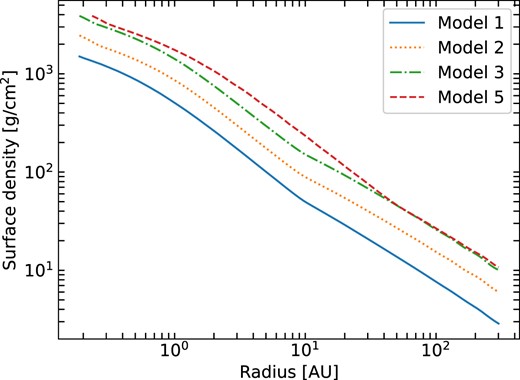
Surface density distributions of models 1, 2, 3, and 5. See Fig. 5 for corresponding mid-plane temperature of the models.
3.3 Images
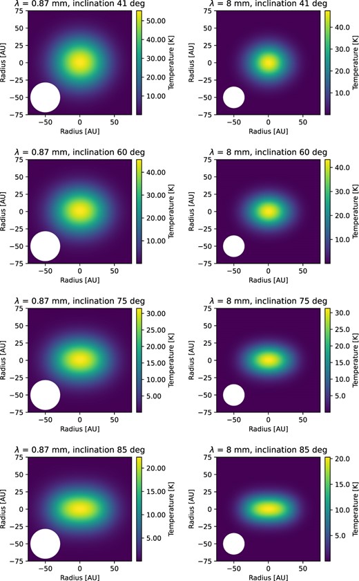
Fig. 7 shows the predicted images of Model 4, viewed at an inclination i = 60°, before and after convolution with Gaussian beams of full width at half-maximum (FWHM) 42 and 30 au at 0.87 and 8 mm, respectively, following K20. This shows that the beam size is a significant factor in how flattened the images appear, particularly at 8mm. However, even with our relatively thick disc and beam convolution, the 0.87 mm image is clearly elongated. Even though the disc is geometrically thicker, because the large optical depth extincts the inner hotter regions, with colder outer parts of the disc becoming more prominent. The images for inclinations 75° and 85° are clearly disc-like (Fig. 8).

Model 4 images viewed at an inclination of i = 60° before and after convolution. White dot in the lower left corner denotes the beam size, the same as used in K20: 42 au for 0.87 mm, and 30 au for 8.1 mm.
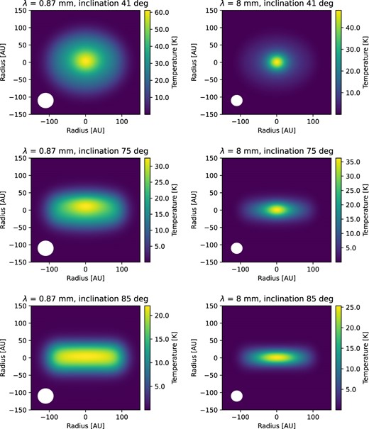
Sequence of convolved images at different inclinations for Model 4, again showing the adopted beam sizes.
The model envelopes do not make a significant contribution to the images. Although the envelopes are very optically thick at wavelengths of ≲ a few µm, absorbing all the radiation from the central source, most of their emission is radiated at far-infrared wavelengths where the optical depths are low, and even less emission is emitted at mm wavelengths. With the small masses at disc scales, (∼1–3 × 10⁻³ M⊙) the emission would be very small compared to that of the discs with masses ∼0.1 M⊙, and with the low mm envelope opacities adopted here, the envelope contributions are completely negligible.
Table 2 lists the total fluxes and peak brightness temperatures of the models. To make a comparison with the observations, in Fig. 9 we show the model results along with fluxes of the HOPS 40x objects plus two highly elongated sources from the VANDAM survey (Tobin et al. 2020). In the left panel of Fig. 9, we focus on the relative behaviour of the Model 4 fluxes as a function of inclination, along with the non-envelope disc model showing the difference envelope backwarming makes. For clarity, we separately show in the right panel all the models with envelopes compared with the HOPS objects.
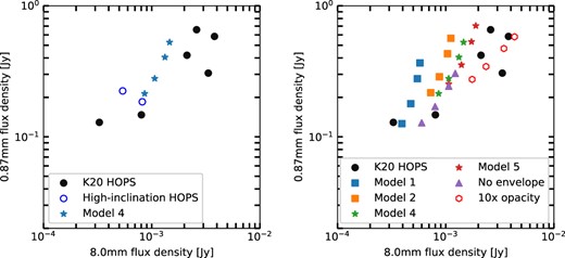
Model fluxes at 0.87 mm versus 8 mm as a function of inclination. Fluxes are shown at inclinations of 85°, 75.5°, 60°, and 41.4°, in ascending order of flux (see Table 2). Left panel: Model 4 fluxes as a function of inclination, plus the equivalent no-envelope disc model, compared with observations of the HOPS 40x sources (filled circles), and two edge-on sources, HOPS 358A and 409 (open circles) from the VANDAM survey (Tobin et al. 2020). Right panel: Fluxes of all disc models with envelopes compared with the HOPS objects. The open hexagons represent results from taking the structure of Model 5 and arbitrarily increasing the opacities at all wavelengths by a factor of 10 arbitrarily, to indicate what would need to change to explain the largest observed fluxes.
Model fluxes and brightness temperatures.
| Model | i | |$F_{0.87\,\textrm {mm}}$|a | |$T_{\mathrm{ b},\mathrm{ m} (0.87\,\textrm {mm})}$|b | |$F_{8\,\textrm {mm}}$|a | |$T_{\mathrm{ b},\mathrm{ m} (8\,\textrm {mm})}$|b |
|---|---|---|---|---|---|
| 1 | 41.4 | 0.37 | 60.0 | 5.8 × 10⁻⁴ | 25.3 |
| 60 | 0.28 | 49.5 | 5.5 × 10⁻⁴ | 26.9 | |
| 75.5 | 0.18 | 29.4 | 4.8 × 10⁻⁴ | 22.8 | |
| 85 | 0.13 | 17.5 | 3.9 × 10⁻⁴ | 16.6 | |
| 2 | 41.4 | 0.57 | 84.0 | 1.1 × 10⁻³ | 45.4 |
| 60 | 0.43 | 67.0 | 1.0 × 10⁻³ | 45.2 | |
| 75.5 | 0.29 | 37.1 | 8.7 × 10⁻⁴ | 37.5 | |
| 85 | 0.22 | 24.3 | 7.3 × 10⁻⁴ | 27.2 | |
| 3 | 41.4 | 0.52 | 74.2 | 1.5 × 10⁻³ | 56.0 |
| 60 | 0.40 | 58.71 | 1.4 × 10⁻³ | 53.8 | |
| 75.5 | 0.27 | 31.06 | 1.1 × 10⁻³ | 41.4 | |
| 85 | 0.20 | 20.32 | 8.7 × 10⁻⁴ | 27.5 | |
| 4 | 41.4 | 0.53 | 60.7 | 1.5 × 10⁻³ | 48.0 |
| 60 | 0.40 | 50.2 | 1.3 × 10⁻³ | 46.0 | |
| 75.5 | 0.28 | 30.6 | 1.1 × 10⁻³ | 36.2 | |
| 85 | 0.21 | 21.9 | 8.6 × 10⁻⁴ | 25.3 | |
| 5 | 41.4 | 0.70 | 79.4 | 1.9 × 10⁻³ | 57.9 |
| 60 | 0.53 | 67.7 | 1.7 × 10⁻³ | 56.8 | |
| 75.5 | 0.35 | 44.0 | 1.4 × 10⁻³ | 47.1 | |
| 85 | 0.25 | 29.0 | 1.1 × 10⁻³ | 30.9 |
Flux in Jy.
Maximum brightness temperatureafter convolution with gaussian beam, in K.
The fluxes systematically decrease as the inclination increases. Because these models are mostly optically thick at 0.87 mm, the fluxes are essentially determined by the disc temperature distribution, and are roughly proportional to cos i as expected, while at the long wavelength the dependence on inclination is weaker because the discs are more optically thin. The VANDAM objects HOPS 358A and 409, which are likely very edge-on discs, are similarly faint. The comparison with the HOPS 40x sources indicates that we are able to roughly match the short-wavelength fluxes but fall short at 8 mm (see Section 4).
Fig. 10 shows cross-cuts through the centre along the equatorial plane for the brightness temperatures of Model 4 as a function of inclination. At low inclinations, the peak Tb is higher at 0.87 mm than at 8 mm, because the long-wavelength emission is more optically thin, but at high inclinations the situation reverses, with the peak Tb (8 mm) > Tb (0.87 mm). This is because when the disc is edge-on, the high optical depth at 0.87 mm means that the emission is arising from the outer, cooler disc.
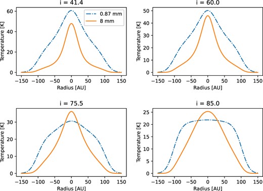
Cross-cut of brightness temperatures at 0.87 and 8 mm for Model 4 at several inclinations. The effect of optical depth at high inclination is apparent in the short-wavelength brightness distribution.
Table 3 lists the major and minor axis FWHM at the two wavelengths for all the models. In general, all the models show significant elongation for inclinations ≳60°.
Measured model FWHM at different inclinations.
| Model | i | 0.87 mma | 0.87 mmb | 8 mma | 8 mmb |
|---|---|---|---|---|---|
| 1 | 41.4 | 90.30 | 75.25 | 44.15 | 40.13 |
| 60.0 | 104.35 | 67.22 | 48.16 | 38.13 | |
| 75.5 | 154.52 | 63.21 | 60.20 | 35.12 | |
| 85.0 | 190.64 | 58.19 | 84.28 | 33.11 | |
| 2 | 41.4 | 90.30 | 77.26 | 44.15 | 40.13 |
| 60.0 | 104.35 | 70.23 | 50.17 | 38.13 | |
| 75.5 | 168.56 | 72.24 | 64.21 | 36.12 | |
| 85.0 | 196.66 | 66.22 | 90.30 | 34.11 | |
| 3 | 41.4 | 90.30 | 77.26 | 48.16 | 42.14 |
| 60.0 | 104.35 | 72.24 | 54.18 | 40.13 | |
| 75.5 | 174.58 | 77.26 | 74.25 | 37.12 | |
| 85.0 | 200.67 | 71.24 | 114.38 | 35.12 | |
| 4 | 41.4 | 120.40 | 96.32 | 50.17 | 44.15 |
| 60.0 | 136.45 | 83.28 | 60.20 | 42.14 | |
| 75.5 | 182.61 | 80.27 | 86.29 | 38.13 | |
| 85.0 | 200.67 | 71.24 | 122.41 | 36.12 | |
| 5 | 41.4 | 128.43 | 101.34 | 52.17 | 46.15 |
| 60.0 | 142.47 | 84.28 | 62.21 | 43.14 | |
| 75.5 | 178.60 | 74.25 | 88.29 | 39.13 | |
| 85.0 | 200.67 | 65.22 | 136.45 | 35.12 |
Note. The FWHM of various models used in the simulations after convolution. aMajor axis, bminor axis, units in au.
4 DISCUSSION
4.1 Fluxes and Tb
While the models are characterized by several parameters, in practice some of these are either relatively unimportant or enter only in combinations. The fluxes and surface brightness distributions at 0.87 and 8.1 mm directly depend upon the disc mass surface density, the dust temperature, and the dust opacity. The dust temperature Td is mostly controlled by the central luminosity L = L* + Lacc; due to the envelope re-emission, Td is only weakly dependent on ρ1 and rc. Thus, as shown in Fig. 4, Td ≈ L1/4r−1/2. For the range of parameters considered here, the disc is optically thick at 0.87 mm, and so the brightness temperatures and fluxes are basically determined by the central luminosity (modulo inclination), which is constrained to be in the range found by Furlan et al. (2016) and K20. Note that the same disc model without a backwarming envelope exhibit dust temperatures a factor of 1.5–3 times smaller at radii ≳4 au (Fig. 2), so the envelope helps to produce larger sub-mm and mm fluxes. (The envelope heating is unimportant at radii ≲1 au because the viscous heating due to accretion dominates.) In general, our models suggest that estimating backwarmed disc temperatures by T ∼ f(L/4πσr2)1/4, with f ∼ 0.7, would be a reasonable first guess in the absence of detailed modelling.
While the models generally span the range of the 0.87 mm fluxes of the K20 objects (Fig. 9), they tend to fall short of the 8 mm fluxes. The discs are more optically thin 8 mm and so, for a given source luminosity, fluxes at this wavelength are sensitive to the disc mass and dust opacity κ8. The surface density in the steady α-disc theory is given by |$\Sigma \propto \dot{M}(\alpha T)^{-1}$|, and since the discs are mostly vertically isothermal, the surface brightness (in the Rayleigh–Jeans limit) is |$I \propto \dot{M}\kappa _8 (\cos i \, \alpha) ^{-1}$|. The fluxes for a fixed outer disc radius show this dependence fairly closely (Fig. 9). Alternatively, one can consider the disc mass to be a parameter, as usually done, in which case the total flux will vary as the usual F ∝ κ8Md〈Td〉, where 〈Td〉 is a suitable average dust temperature. In any case, the only means to increase the 8 mm fluxes substantially would be to either increase the disc mass or the dust opacity, or both.
The difficulty with adopting larger disc masses is that our models are already at the limit of gravitational instability (GI) (Table 1), with the Toomre Q approaching unity in the outer regions (see Fig. 11). Note that the disc model without an envelope corresponding to Model 4 is not only systematically fainter, it is also much more gravitationally unstable because of the lower temperatures. We also point out that our calculations assumes a central mass of 0.5–1.0 M⊙. Because |$Q \propto M_*^{1/2}$|, adopting a lower mass closer to the typical peak of the stellar initial mass function, perhaps more likely for such young objects, would make Q even smaller.
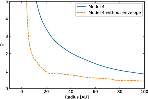
Variation of Toomre Q with radius for Model 4, with or without envelope.
Sequence of images at different inclinations for Model 4, but with the disc truncated at 30 au.
On the other hand, our adopted opacity at 8 mm, |$\sim 0.42 \, {\rm cm^2\, g^{-1}}$|, is already a factor of 3 larger than that used by K20. Consistent with this, K20 estimated masses of 0.45–1.2 M⊙ using an 8 mm opacity about three times smaller than ours for four brightest objects, which led to their estimated masses being a similar factor larger. Thus, if we had adopted the K20 opacities, the disc models would have to be extremely gravitationally unstable to achieve the same sub-mm and mm fluxes.
Another problem is that our models cannot exhibit a higher peak Tb at 8 mm than at 0.87 mm, as found by K20 for four of the six sources, unless the disc is edge-on. It seems unlikely that the estimated calibration errors of ∼10 per cent can account for this discrepancy. Instead, we suspect that there is an additional central component of free–free emission from jets, as frequently seen in protostellar objects (Anglada et al. 1998). In support of this suggestion, we note that K20 found evidence for bipolar molecular outflows in four of the six objects. However, assuming that the jets contribute only to the central unresolved structure, our estimates indicate that only a modest fraction of the flux shortfall of our models can be attributed to free–free emission.
4.2 Geometry
While our envelope-irradiated disc models appear less flattened than non-envelope-heated discs, they still predict a significant asymmetry for inclinations ≳60° (see Table 3), which would occur for half of the objects assuming a random distribution of inclinations. This asymmetry is not consistent with the K20 observations of HOPS 400A, 402, and 403, where as K20 state ‘The aspect ratios of the irregular structures are close to 1, particularly when considering the outer contours of the 0.87 mm emission’.
We find that the relatively low optical depths of the envelopes at far-infrared wavelengths, where most of the radiation emerges, limit the amount of radiative trapping, which in turn limits the envelope temperatures and the amount of backwarming. The resulting increase in temperatures in the outer discs by factors of ∼2 increases the scale heights only by factors of ∼21/2 (H ∝ T1/2).
We have not explored whether a different dust size distribution in the envelopes could increase backwarming. While there is some evidence for dust growth to mm sizes in protostellar envelopes (Miotello et al. 2014; Galametz et al. 2019), the observations are difficult and there are theoretical arguments against such large grain growth in envelopes (Silsbee et al. 2022). A further problem is that the SEDs of typical protostars and some of the HOPS 40x sources do not suggest large dust. As shown in Fig. 1, the usual power-law dust size distributions with large enough maximum sizes to provide sufficient 8 mm opacity result in strongly weakening the 10 and 18 µm silicate features, if not entirely eliminating them, inconsistent with observations of HOPS 400 and 403 (Furlan et al. 2016).
In any event, the models show 0.87 mm brightness temperatures (assuming a large enough disc dust opacity) that are comparable to the K20 observations, indicating that the resulting temperature structures are realistic.
5 MORPHOLOGY
Any attempt to explain the complex morphology of the K20 objects is beyond the scope of this paper, which addresses only steady-state, axisymmetric models with self-consistent vertical density and temperature structures. GI might produce spiral arms, although this would not necessarily result in less-flattened discs. Another possibility is filamentary infall impacting discs, for which there is observational evidence (Tobin et al. 2010; Chou et al. 2016; Pineda et al. 2020, 2023; Valdivia-Mena et al. 2022), and is predicted by several simulations (Kuffmeier, Haugbølle & Nordlund 2017; Kuffmeier, Calcutt & Kristensen 2019; Kuznetsova, Hartmann & Heitsch 2019, 2020; Wurster, Bate & Price 2019). Finally, gravitational perturbations by companion protostars, as seen in the protostellar triple system L1448 IRS3B (Tobin et al. 2016), seem possible. In this connection, it is noteworthy that HOPS 400AB is a binary system, and there is some suggestion of a companion in HOPS 403 (K20). In any case, hydrodynamical simulations are needed to test these alternative hypotheses.
6 SUMMARY
We have developed steady accretion disc models with self-consistent calculations of the vertical hydrostatic equilibrium, which include irradiation of the discs by infalling envelopes. The discs become significantly hotter because of the envelope backwarming, increasing long-wavelength dust emission, but only modestly increasing disc scale heights. Comparison of our models to observations of the unusual HOPS 40x sources indicates that backwarming in principle can help explain the bright sub-mm and mm fluxes of these objects, but cannot resolve the morphological issues raised by K20.
Our models, though relatively simple, show that envelope backwarming can be important in setting the temperatures of protostellar discs. Further progress requires exploration by more complex, time-dependent models of protostellar disc formation and fragmentation, such as those of Bate (2011), Wurster et al. (2019), and Lee, Charnoz & Hennebelle (2021).
Acknowledgement
This paper significantly benefited from comments by Nicole Karnath, John Tobin, Tom Megeath, and Amy Stutz. This work was supported in part by the University of Michigan.
DATA AVAILABILITY
The models and associated data will be provided upon reasonable request to the authors.
Footnotes
For θ ≳ 1.1, sin(π/2 − θ) ∼ π/2 − θ ∼ z/R, where the latter are the height above the disc and the radius in cylindrical coordinates.
