


ABSTRACT
Magnetized hypermassive neutron stars (HMNSs) have been proposed as a way for neutron star mergers to produce high electron fraction, high-velocity ejecta, as required by kilonova models to explain the observed light curve of GW170817. The HMNS drives outflows through neutrino energy deposition and mechanical oscillations, and raises the electron fraction of outflows through neutrino interactions before collapsing to a black hole (BH). Here, we perform 3D numerical simulations of HMNS–torus systems in ideal magnetohydrodynamics, using a leakage/absorption scheme for neutrino transport, the nuclear APR equation of state, and Newtonian self-gravity, with a pseudo-Newtonian potential added after BH formation. Due to the uncertainty in the HMNS collapse time, we choose two different parametrized times to induce collapse. We also explore two initial magnetic field geometries in the torus, and evolve the systems until the outflows diminish significantly (|$\sim\!\! 1\!\! - \!\!2\ \mathrm{s}$|). We find bluer, faster outflows as compared to equivalent BH–torus systems, producing M ∼ 10−3 M⊙ of ejecta with Ye ≥ 0.25 and v ≥ 0.25c by the simulation end. Approximately half the outflows are launched in disc winds at times |$t\lesssim 500 \ \mathrm{ms}$|, with a broad distribution of electron fractions and velocities, depending on the initial condition. The remaining outflows are thermally driven, characterized by lower velocities and electron fractions. Nucleosynthesis with tracer particles shows patterns resembling solar abundances in all models. Although outflows from our simulations do not match those inferred from two-component modelling of the GW170817 kilonova, self-consistent multidimensional detailed kilonova models are required to determine whether our outflows can power the blue kilonova.
1 INTRODUCTION
Neutron star (NS) mergers are long thought to be a site for the creation of r-process elements and the production of kilonovae, powered by their radioactive decays (Lattimer & Schramm 1974; Paczynski 1986; Eichler et al. 1989; Li & Paczyński 1998; Metzger et al. 2010). This was confirmed following the coincident gravitational wave and kilonova detection, GW170817 (Abbott et al. 2017a, b), which indicated broad agreement between many observations and theoretical predictions (e.g. Chornock et al. 2017; Cowperthwaite et al. 2017; Drout et al. 2017; Tanaka et al. 2017; Tanvir et al. 2017).
However, many details of the kilonova and r-process production have not yet been resolved. One of the outstanding issues comes from multicomponent light-curve fits using analytical ejecta models to kilonova observations that predict a fast (v ≳ 0.25c), optical ‘blue’ component composed of high electron fraction (Ye) material, as well as a slower (v ∼ 0.1c) infrared ‘red’ component containing most of the ejecta mass with Ye ≤ 0.25 (e.g. Kasen et al. 2017; Perego, Radice & Bernuzzi 2017; Villar et al. 2017). While these multicomponent models are simple to apply, multidimensional radiative transfer models including accurate nuclear heating rates, thermalization efficiencies, and opacities are more physically motivated. Some of these more advanced kilonova models indicate that in order to recreate the kilonova of GW170817, the disc wind may require velocities as low as v ∼ 0.05c (e.g. Bulla 2023; Ristic et al. 2023). 3D magnetohydrodynamic (MHD) numerical simulations of black hole (BH) accretion discs from NS mergers have difficulty producing a massive, high-velocity blue component, making the need apparent for more detailed kilonova models, an additional component in NS merger simulations, or both (e.g. Metzger, Thompson & Quataert 2018; Darbha & Kasen 2020; Kawaguchi, Shibata & Tanaka 2020; Barnes et al. 2021; Heinzel et al. 2021; Korobkin et al. 2021; Kawaguchi et al. 2022, 2023; Bulla 2023; Just et al. 2023; Ristic et al. 2023).
Due to differences in requisite physics and computational costs, many 3D numerical simulations split the evolution of NS mergers into two or more phases, usually modelling either the inspiral and merger of the two stars, often in general relativistic hydrodynamics (GRHD, e.g. see Radice, Bernuzzi & Perego 2020; Perego, Thielemann & Cescutti 2021; Janka & Bauswein 2022; Rosswog & Korobkin 2022, for recent reviews), or the post-merger phase consisting of a torus around a remnant compact object in (general relativitistic – GR)MHD (a BH or an NS; e.g. Hossein Nouri et al. 2018; Siegel & Metzger 2018; Christie et al. 2019; Fernández et al. 2019a; Miller et al. 2019; Fahlman & Fernández 2022; Just et al. 2022; Curtis et al. 2023b), although many recent works deviate from this structure (see e.g. Ciolfi et al. 2019; Hayashi et al. 2022; Lopez Armengol et al. 2022; Just et al. 2023; Kiuchi et al. 2023).In equal-mass NS mergers, the secular wind stage is thought to provide the majority of the mass outflow responsible for powering the kilonova, making simulations of this phase crucial for resolving discrepancies with kilonova models of GW170817 (e.g. Wu et al. 2016; Metzger et al. 2018; Radice et al. 2018; Margalit & Metzger 2019; Fujibayashi et al. 2020b).
The above simulations of BH–torus systems suggest that winds from the disc can eject sufficient mass to power the red kilonova, but are lacking enough mass in high electron fraction (Ye ≳ 0.25), high-velocity (v ≳ 0.25c) outflows to create the blue kilonova. Several studies point to the formation of a short-lived hypermassive NS (HMNS) as a resolution to the lack of this ejecta (e.g. Metzger et al. 2018; Fahlman & Fernández 2022; Combi & Siegel 2023a; Curtis et al. 2023a). An HMNS formed in a merger is supported against collapse to a BH through additional pressure provided by differential rotation and thermal effects. As the differential rotation is removed through angular momentum transport, and thermal energy is lost to neutrinos (e.g. Duez et al. 2006; Kaplan et al. 2014; Hanauske et al. 2017; Ciolfi et al. 2019; Bernuzzi 2020; Janka & Bauswein 2022, and references therein), the HMNS will collapse on a time-scale of |$t \sim 1\!\!-\!\!100 \ \mathrm{ms}$|. The results of previous 3D simulations and 2D viscous hydrodynamic simulations indicate that during the time it is present, the HMNS will drive high electron fraction winds via neutrino absorption, magnetic effects, and mechanically driven oscillations.
A complete model of the HMNS and torus system requires inclusion of GR, MHD, neutrino transport, a realistic nuclear equation of state (EOS), and time-scales long enough to capture the ejecta from both the early HMNS and late-time torus winds (∼1 s). In particular, the HMNS phase of the merger requires very high spatial resolutions in 3D to resolve the wavelength of the most unstable mode of the magnetorotational instability (MRI) within the HMNS and torus, and ensure that the MRI dynamo is not suppressed through axisymmetry (Cowling 1933).
In practice, detailed long-term modelling of these effects is eschewed in the name of computational costs, and instead has been mostly simulated in reduced dimensionality in combination with parametrized angular momentum transport (e.g. Lippuner et al. 2017; Fahlman & Fernández 2018; Shibata, Fujibayashi & Sekiguchi 2021a; Fujibayashi et al. 2023; Just et al. 2023), with a parametrized dynamo (Shibata, Fujibayashi & Sekiguchi 2021b), or in 3D viscous simulations (Perego et al. 2014; Foucart et al. 2020; Nedora et al. 2021).
Currently, there are few simulations of 3D MHD HMNS systems (e.g. Kiuchi, Kyutoku & Shibata 2012; Siegel, Ciolfi & Rezzolla 2014; Ciolfi & Kalinani 2020; Mösta et al. 2020; de Haas et al. 2022; Combi & Siegel 2023a; Curtis et al. 2023a), with only one simulation lasting ∼1 s (Kiuchi et al. 2023). The varying input neutrino physics, HMNS lifetimes, and magnetic field strengths and orientations result in little consensus on the composition, mass, velocities, and ejection mechanisms for their outflows.
Here, we present long-term 3D MHD numerical simulations of HMNS and torus systems, starting from varying idealized initial conditions. We utilize a (pseudo-)Newtonian potential (Artemova, Bjoernsson & Novikov 1996), the nuclear APR EOS (Schneider et al. 2019), and a leakage/absorption scheme to handle energy deposition and lepton number change from neutrinos, as described in Section 2. In Section 3, we examine our outflows in the context of powering a kilonova while ignoring effects from relativistic jets, which we are unable to model without full GR. In Section 4, we compare to other works, and in Section 5 we conclude. Appendix A describes updates to our previously used neutrino scheme to handle an HMNS fully contained in the computational domain.
2 METHODS
2.1 Numerical MHD
We use a modified version of the flash4.5 code to run our MHD simulations in non-uniform 3D spherical coordinates. A full description (along with code verification tests) is provided in Fahlman & Fernández (2022); here, we give a brief overview. The code solves the Newtonian conservation equations for mass, momentum, energy, and lepton number, as well as the induction equation:
where ρ is the density, v is the velocity, B is the magnetic field (including a normalization factor |$\sqrt{4\pi }$|), Ye is the electron fraction, and E is the total specific energy of the fluid:
We denote the specific internal energy by eint, and P is the sum of gas and magnetic pressure:
We use the constrained transport method (Evans & Hawley 1988) to preserve the solenoidal condition (∇ · B = 0) while evolving the induction equation. We include source terms from the self-gravitating potential of the fluid, Φ, neutrino heating and cooling, Qnet, and lepton number change, Γnet. Our self-gravity scheme utilizes the Newtonian multipole solver of Müller & Steinmetz (1995), as implemented in Fernández, Margalit & Metzger (2019b). After the HMNS collapses into a BH, we add a point source term with the mass of the remnant to the zeroth moment of the multipole expansion using the Artemova potential (Artemova et al. 1996). We close the equations with the hot APR EOS of Schneider et al. (2019). The additional source terms from our neutrino scheme are calculated using a three-species, two-source, lightbulb-leakage scheme (Metzger & Fernández 2014; Lippuner et al. 2017; Fernández et al. 2022). We use local emission rates from Bruenn (1985) for neutrino production from charged-current interactions, and the rates from Ruffert et al. (1997) for plasmon decay, nucleon–nucleon bremsstrahlung, and pair processes. We take into account absorption due to charged-current weak interactions from electron-type neutrinos and antineutrinos emitted by the central HMNS and by a ring within the torus. The implementations of our neutrino source terms are detailed in Appendix A.
2.2 Initial torus
We initialize our simulations with a constant specific angular momentum, entropy, and composition torus in hydrostatic equilibrium with a point mass remnant in a Newtonian potential. Generating the torus requires choosing input parameters, which we set according to inferred values from GW170817 (see e.g. Abbott et al. 2017c; Shibata et al. 2017; Fahlman & Fernández 2018). For all our simulations, we set a remnant mass of 2.65 M⊙, torus mass of 0.1 M⊙, radius of density maximum at |$50 \ \mathrm{km}$|, entropy of |$s = 8k_\mathrm{ b} \ \mathrm{ per} \ \mathrm{baryon}$|, and Ye = 0.1. This results in a torus with an initial maximum density |$\rho _{\rm max} = 8\times 10^{10} \ \mathrm{g\, cm}^{-3}$|. Matter initialized in the torus is flagged as torus material using a passive mass scalar that is advected with the flow. We neglect the self-gravity of the torus in the initialization process, as the system mass is dominated by the remnant. We additionally neglect spatial variations in the composition and entropy, which have been found to make small (|$\sim\!\! 10~{{ \rm per\, cent}}$|) differences in the outflows around BH accretion discs (Fernández et al. 2017; Fujibayashi et al. 2020a, b; Most et al. 2021; Nedora et al. 2021).
The torus is then threaded with a magnetic field. We choose magnetic field configurations that cover possible geometries found in magnetized merger simulations, which generally yield a combination of (turbulent) toroidal and poloidal fields. Due to the high-resolution requirements to capture the mechanisms for amplifying the field at merger and within the remnant plus torus (e.g. the Kelvin–Helmholtz instability and MRI), we start with field strengths that assume that growth and saturation have been reached, allowing us to resolve the smallest growing wavelength of the MRI with our grid (see Fig. 1 and Section 2.5). These field strengths are similar to those found in merger simulations that use sub-grid models to resolve these effects (e.g. Aguilera-Miret et al. 2023). For models that specify a poloidal field geometry, this is initialized using an azimuthal vector potential that follows the density,
where ρ0 = 0.009ρmax is the cut-off density used to ensure that the field is embedded in the torus. This results in a poloidal (‘SANE’) field topology (Hawley 2000). The field is normalized to be dynamically unimportant, with an average plasma β of
resulting in a maximum field strength of |$|B_\mathrm{ r}| \sim |B_\theta | \sim 4\times 10^{14}\ \mathrm{G}$|. Models with a toroidal field geometry are initialized as
where |$B_0 = 5 \times 10^9\ \mathrm{G}/(\mathrm{g\, cm}^{-3})$|. This results in nearly constant azimuthal magnetic field embedded within the torus, which tapers off as a function of the density profile. The field has a maximal value of |$8 \times 10^{14}\ \mathrm{G}$|, and an average strength of |$\sim\!\! 2\times 10^{14} \ \mathrm{G}$|.
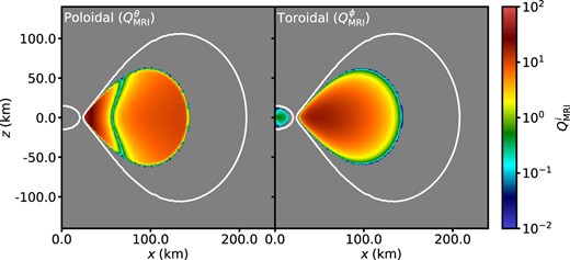
Slices of the MRI quality parameter |$(Q_\mathrm{MRI}^i = \lambda _\mathrm{MRI}^i/\Delta \ell _i)$|, where |$\lambda _\mathrm{MRI}^i$| is the wavelength of the most unstable mode of the MRI and Δℓi is the cell width in the specified ith direction. Slices are in the x–z (ϕ = 0) plane of the Bpol-t30 and Btor-t30 models at initialization. The solid white lines mark the |$3\times 10^8\ \mathrm{g\, cm}^{-3}$| density contour, corresponding to near the edge of the torus and HMNS. Grey colour denotes regions without any magnetization in the relevant direction. The field is well embedded within the torus, and is generally resolved by at least 10 cells. The toroidal field in the HMNS is not well resolved due to the high densities, and as such we do not expect to resolve magnetized outflows driven by MRI turbulence in the remnant.
2.3 Initial HMNS
Our torus orbits a stable equilibrium model of an azimuthally symmetric, differentially rotating NS. We find 2D HMNS thermodynamic profiles using the code newtneut, a reduced version of the code drns (Stergioulas & Friedman 1995). newtneut generates differentially rotating high-density stars in the Newtonian limit, taking a central density, rotation law, and EOS as input, and utilizing the self-consistent field method of Hachisu (1986, HSCF) to generate thermodynamic profiles for a differentially rotating non-relativistic star. The equilibrium equation that the HSCF method solves is
where Φg is the (Newtonian) gravitational potential, and Ω is a choice of rotation profile dependent on rcyl, the cylindrical radial coordinate. We use the well-studied j-const rotation law (Hachisu 1986; Baumgarte, Shapiro & Shibata 2000):
where Ω0 is the central rotation rate, |$\hat{A} = A/r_\mathrm{ e}$| is a scaling constant that sets the amount of differential rotation, and |$\hat{r} = r/r_\mathrm{ e}$| is the radial coordinate normalized to the equatorial radius of the star. We use a uniform spherical grid with a resolution of (Nr × Nθ) = (200 × 200) to generate one quadrant of the NS, and then assume azimuthal and equatorial symmetries to generate the rest of the star. The HSCF method requires finding the quantity ∫ρ−1dP, which can be obtained from the enthalpy,
as long as our star satisfies the barotropic condition TdS = 0. We choose to generate stars of constant entropy, so that neutrino emission is not suppressed by a zero temperature initial condition. Our choice of constant angular momentum differential rotation law and constant entropy are not entirely correct for the remnant of an NS–NS merger, as more realistic NSs follow a rotation law that peaks away from the central density (e.g. Hanauske et al. 2017; Iosif & Stergioulas 2022), and have varying spatial entropy (e.g. Most et al. 2021; Nedora et al. 2021).
The generated HMNS has a mass 2.65 M⊙, entropy |$s= 2 k_\mathrm{B} \ \mathrm{ per} \ \mathrm{baryon}$|, with |$\hat{A}=0.5$|, and the central rotation rate chosen such that the ratio of polar to equatorial radius is rp/re = 0.75. This makes a star with a maximal equatorial radius and central rotation rate of 23.5 km and |$3780\ \mathrm{rad\, s}^{-1}$|, respectively, corresponding to a period of |$\sim\!\! 1.6\ \mathrm{ms}$|. The thermodynamically consistent axisymmetric density, electron fraction, temperature, internal energy, and rotational velocity profile output from newtneut are read into flash, and the relevant quantities are linearly interpolated to the cell centres to create our initial HMNS. Like the torus, HMNS matter is also flagged using a passively advected mass scalar. In all our runs, we embed the HMNS with a dynamically unimportant axisymmetric toroidal field that vanishes as we approach the origin, as motivated by merger simulations (Shibata et al. 2021b). The HMNS field is given by
where |$\rho _0 = 5\times 10^{13}\ \mathrm{g\, cm}^{-3}$| is 1/10 the central density of the HMNS, and the constant |$B_{\mathrm{ NS}} = 8\times 10^{4}\ \mathrm{G}/(\mathrm{g\, cm}^{-3})$| is set such that the total magnetic energy within the NS is |$2\times 10^{47}\ \mathrm{erg}$|. We note that the magnetic field geometry is no longer toroidal by |$t \sim 5\ \mathrm{ms}$|, as it is modified by the dynamics inside the HMNS.
2.4 Tracer particles
Tracer particles are used to track nucleosynthesis in post-processing. We initialize 10 000 tracer particles by placing them into pseudo-random positions within the domain, following the density distribution, where the density falls in the range |$10^6 \ \mathrm{g\, cm}^{-3} \le \rho \le 10^{13} \ \mathrm{g\, cm}^{-3}$| and the atmospheric fraction is 0. This ensures that the particles are embedded within the torus and the edges of the HMNS, but also that few are trapped in the HMNS when it collapses. Particles are then advected with the fluid flow, and the history of any particles that make it past a fixed extraction radius rout is used in nucleosynthesis calculations. The latter are carried out with the publicly available nuclear reaction network skynet (Lippuner & Roberts 2017), with the same settings as Fernández, Foucart & Lippuner (2020).
2.5 Computational domain
We solve the MHD equations in spherical polar coordinates (r, θ, ϕ) on a domain initially ranging from an inner boundary at |$r_\mathrm{min}=0\ \mathrm{km}$| to an outer radius |$r_\mathrm{max}=10^5\ \mathrm{km}$|, located far away from the central remnant. Both the polar (θ) and azimuthal (ϕ) domains subtend an angle from 0 to π, creating a hemisphere.
Upon collapse of the HMNS, we excise an integer number of cells covering a radial region interior to a new radius rmin, located approximately halfway between the event horizon and innermost stable circular orbit (ISCO) of the newly formed BH. To preserve the total number of radial cells in the grid, the domain is expanded outwards in radius by the same number of cells removed around the origin, with the new cells filled with ambient medium. Since no ejecta has reached the outer radial boundary at the collapse times, this results in no effective change to the simulation outside rmin. For all models, this results in a post-collapse value of |$r_\mathrm{min} = 15.4\ \mathrm{km}$| and an outer boundary at |$r_\mathrm{max} = 5.23 \times 10^5\ \mathrm{km}$|.
We use a logarithmic grid in the radial direction, a grid evenly spaced in cos θ in the polar direction, and uniform spacing in azimuth. To avoid issues with time stepping close to the singularity, we make the innermost radial cell large, with a size of |$3\ \mathrm{km}$|, encompassing the inner ∼13 per cent of the HMNS radius. We set our polar and azimuthal resolutions such that the initial wavelength of the most unstable mode of the MRI within the torus is resolved with ∼10 cells, and set a radial resolution to get approximately square cells in the mid-plane of the torus. This results in a mesh size of (Nr × Nθ × Nϕ) = (580 × 120 × 64), focused towards the mid-plane of the disc, with Δr/r ∼ 0.018, min(Δθ) ∼ 0.017, and Δϕ ∼ 0.1. We show the MRI quality factor (Sano et al. 2004) for both our initial set-ups in Fig. 1.
The boundary conditions of our domain are periodic in the azimuthal direction, and reflecting along the polar axes. The outer radial boundary is set to outflow, while the inner radial boundary is initially reflecting while the HMNS survives. After collapse, we set the inner radial boundary to outflow so that matter can accrete on to the BH.
2.6 Floor
To avoid issues with convergence, finite-volume codes implement density floors. We impose a spatial and temporal varying floor to prevent computationally unfeasible low time-steps in magnetized regions near the inner boundary and rotation axis, while not affecting dynamics of the outflows. We implement the functional form used in Fahlman & Fernández (2022):
where |$\rho _\mathrm{sml} = 2\times 10^4\ \mathrm{g\, cm}^{-3}$|. When the code reaches a density below the floor value in that cell, we add atmospheric material to raise it back up. Identical floors are implemented for pressure and internal energy, with the respective scaling constants |$P_\mathrm{sml} = 2\times 10^{14}\ \rm{erg\,cm}^{-3}$| and esml = 2 × 10¹¹ erg g−1. In the magnetized polar funnel close to the BH, we find that this restriction is often too low, but raising the floor results in unphysical effects in important areas of the flow. To address this, we impose an alternative floor on the density only that is dependent on the magnetization, as in Fernández et al. (2019a):
where we find ζ = 2, a reasonable value to increase the time-step in the magnetized funnel, without affecting the dynamics in the disc. We then impose the floor
2.7 Models
Our models are summarized in Table 1. We choose parameters for the torus and HMNS, which are the most likely properties of the remnant + disc system for GW170817 (e.g. Abbott et al. 2017c; Shibata et al. 2017; Fahlman & Fernández 2018), while varying the lifetime of the remnant and the initial field topology.
Simulation parameters. From left to right, they list the name of the model, the mass of the remnant, the lifetime of the HMNS, the initial mass of the torus, the peak magnetic field strength in the torus, and the magnetic field geometry.
| Model | Mremnant | τHMNS | Mt | ||B|| | B |
|---|---|---|---|---|---|
| (M⊙) | (ms) | (M⊙) | (G) | geom | |
| Bpol-t30 | 2.65 | 30 | 0.10 | 4 × 10¹⁴ | pol |
| Bpol-t100 | 100 | ||||
| Btor-t30 | 30 | tor | |||
| Btor-t100 | 100 |
| Model | Mremnant | τHMNS | Mt | ||B|| | B |
|---|---|---|---|---|---|
| (M⊙) | (ms) | (M⊙) | (G) | geom | |
| Bpol-t30 | 2.65 | 30 | 0.10 | 4 × 10¹⁴ | pol |
| Bpol-t100 | 100 | ||||
| Btor-t30 | 30 | tor | |||
| Btor-t100 | 100 |
2.8 Outflows
We calculate the total outflow by temporally integrating the mass flux passing through an extraction radius rout,
where |$A_r = \iint r^2\sin \theta \mathrm{d}\theta \mathrm{d}\phi$| is the area of the cell face. After testing various extraction radii, we choose |$r_\mathrm{out} = 1000\ \mathrm{km}$| as a radius where unbound matter has minimal interaction with the atmosphere, which can impact the energy of the ejecta, as well as being far away from the edges of the viscously spreading disc at late times, but close enough for most ejecta to cross during the simulation time. Matter is considered unbound if it has a positive Bernoulli parameter at the extraction radius,
and we discount any ‘atmospheric’ matter that is present due to the requirement of the non-zero floor (Section 2.6).
We tabulate the ejecta in terms of total, ‘blue’ (Ye ≥ 0.25), and ‘red’ (Ye < 0.25) outflows, based on the characteristic division between lanthanide-poor and lanthanide-rich materials found in parametric nuclear network calculations (e.g. Kasen, Fernández & Metzger 2015; Lippuner & Roberts 2015). The mass-weighted averages of electron fraction and radial velocity,
are shown alongside the mass outflows in Table 2.
Mass ejection from all models. Columns show, from left to right, the model name, maximum simulation time, total unbound mass ejected at |$r_\mathrm{out} = 1000\ \mathrm{km}$| using the Bernoulli criterion, mass ejected that is composed of HMNS material, |$\dot{M}_\mathrm{out}$|-weighted average electron fraction and radial velocity, as well as unbound ejected mass, average electron fraction, and radial velocity broken down by electron fraction (superscript blue – lanthanide poor: Ye ≥ 0.25, red – lanthanide rich: Ye < 0.25).
| Model | tmax | Mout | |$M_\mathrm{out}^\mathrm{HMNS}$| | 〈Ye〉 | 〈vr〉 | |$M^\mathrm{blue}_\mathrm{out}$| | |$\langle Y_\mathrm{ e}^\mathrm{blue}\rangle$| | |$\langle v^\mathrm{blue}_r \rangle$| | |$M^\mathrm{red}_\mathrm{out}$| | |$\langle Y_\mathrm{ e}^\mathrm{red} \rangle$| | |$\langle v^\mathrm{red}_r \rangle$| |
|---|---|---|---|---|---|---|---|---|---|---|---|
| (s) | (10−2 M⊙) | (10−2 M⊙) | (c) | (10−2 M⊙) | (c) | (10−2 M⊙) | (c) | ||||
| Bpol-t30 | 1.31 | 6.309 | 0.012 | 0.235 | 0.057 | 2.073 | 0.295 | 0.125 | 4.236 | 0.206 | 0.024 |
| Btor-t30 | 2.00 | 5.992 | 0.026 | 0.226 | 0.035 | 1.494 | 0.305 | 0.091 | 4.498 | 0.200 | 0.017 |
| Bpol-t100 | 0.75 | 4.790 | 0.012 | 0.223 | 0.059 | 1.619 | 0.294 | 0.120 | 3.171 | 0.186 | 0.029 |
| Btor-t100 | 0.70 | 1.886 | 0.021 | 0.213 | 0.050 | 0.510 | 0.317 | 0.109 | 1.376 | 0.175 | 0.028 |
Throughout this paper, we identify material that is ejected through different mechanisms using the energy and entropy of the ejecta. Regions with large neutrino heating source terms are imparted with large internal energies and entropies, which we identify as neutrino-driven winds. Conversely, fast, low-entropy material from regions with small neutrino heating source terms and high magnetization is identified as purely MHD driven. Passive tracer particles are also used to track the source terms applied to them as they are ejected and corroborate the identification of different mass ejection mechanisms.
3 RESULTS
3.1 Overview of HMNS outflows
We show the mass outflow rates and cumulative mass outflows for all models in Fig. 2. Mass ejection is dominated by the torus (|$\gtrsim\!\! 99~{{ \rm per\, cent}}$|), although the HMNS provides additional channels. During the first |$\sim\!\! 30\ \mathrm{ms}$| of evolution, the HMNS ejects mass through mechanical oscillations, which induce noticeable pressure waves in the torus. Viscous spreading from the action of the MRI and the HMNS oscillations drives the centre of mass of the torus out from 〈rCM〉 ∼ 10 km by a factor of 2–4, depending on the initial field geometry and lifetime of the HMNS, and the lower density edges of the torus develop turbulent structures.
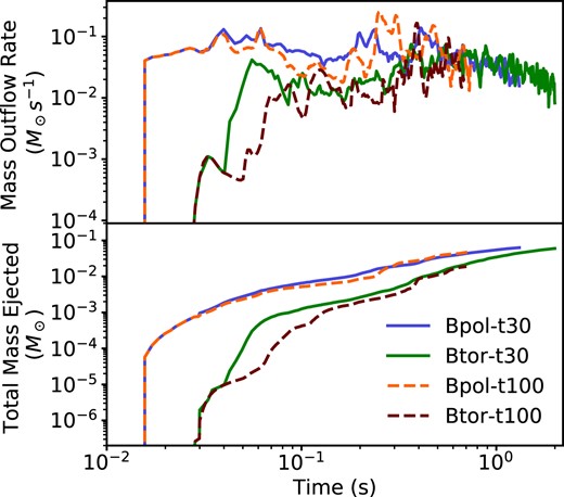
Top: Unbound mass outflow rates in our simulations at a radius of |$r=1000\ \mathrm{km}$|. Bottom: Cumulative ejected mass in the simulations.
The initial sharp increase in mass outflow rate shown in Fig. 2 is dominated by ejection through MHD stresses in the torus that are dependent on the initial magnetic field geometry, as seen in BH–tori simulations (Christie et al. 2019; Siegel, Barnes & Metzger 2019; Fahlman & Fernández 2022; Curtis et al. 2023b). The large-scale poloidal field generates characteristic ‘wings’ in the first |$\sim\!\! 30\ \mathrm{ms}$|, whereas the toroidal field takes an additional time (|$\sim\!\! 50\ \mathrm{ms}$|) for dynamo action to convert the geometry into large-scale poloidal structures, which then drives outflows. Material ejected through MHD stresses tends to have a wide range of electron fractions and velocities, spanning Ye ∼ 0.1–0.5, and v ∼ 0.05–0.6c. The majority of MHD- and neutrino-driven winds are imprinted in the levels showing |$t \lesssim 500\ \mathrm{ms}$| in the cumulative mass histograms of Fig. 3, with the transition to purely thermally driven outflows (Section 3.2) happening around the |$500\ \mathrm{ms}$| mark.
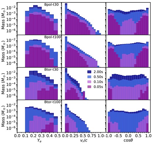
Total unbound mass ejected by our simulations at the extraction radius, binned into electron fraction Ye, radial velocity vr, and polar angle θ. The bin sizes are ΔYe = 0.05, Δvr/c = 0.05, and Δcos θ = 0.1, where cos θ = 0 is the mid-plane. Accounting for the time taken for the ejecta to reach the extraction radius (|$r_\mathrm{out}/v_\mathrm{r} \lesssim 70\, \mathrm{ms}$|), the 0.1, 0.5, and 2.0 s bins are populated by ejecta launched post-collapse in the Bpol-t30 and Btor-t30 models. Similarly, the 0.5 and 2.0 s bins are comprised of mainly post-collapse ejecta in the Bpol-t100 and Btor-t100 models.
Also in the first |$30\!\!-\!\!100\ \mathrm{ms}$|, depending on the HMNS lifetime, high-entropy (|$s\sim 100k_\mathrm{B} \ \mathrm{ per} \ \mathrm{baryon}$|), magnetically driven and neutrino-driven outflows are driven from the edges of the torus, which achieves electron fractions Ye ≳ 0.3 and velocities v ≳ 0.5c. As illustrated by the angular histograms of Fig. 3, this material is preferentially ejected in a cone of opening angle 50°, centred on the angular momentum axis (the polar regions). It is dominated by matter from the torus, with ∼30 times more ejecta from the torus than from the HMNS.
Fig. 4 and the leftmost panels of Fig. 5 show the matter density around the HMNS just before collapse. A magnetized funnel is formed while the HMNS survives, but there remains a significant amount of matter in the funnel with densities |$\rho \sim 10^6 \ \mathrm{ to} \ 10^8\ \mathrm{g\, cm}^{-3}$| from HMNS oscillations and accreting matter, leading to the absence of steady-state, high-velocity, collimated magnetic ‘tower’ outflows from the HMNS (the so-called baryon loading problem). After collapse of the HMNS, the polar regions become evacuated of matter and sit on our imposed density floor, so we cannot draw conclusions on whether or not matter would be launched post-collapse.
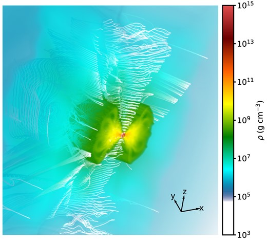
Volume rendering of the Bpol-t30 run at |$t=30\ \mathrm{ms}$|, right before the HMNS collapse to a BH is initiated. Colours show the density with increasing transparency as the density decreases. The visible outer edge of the torus in green (|$\sim\!\! 10^{8} \ \mathrm{g\, cm}^{-3}$|) is located |$\sim\!\! 350 \ \mathrm{km}$| from the remnant in the mid-plane. Magnetic field streamlines are shown in white. Note the formation of a lower density, highly magnetized funnel along the spin axis of the HMNS.
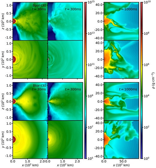
Slices of density in the x–z (ϕ = 0, polar) and x–y (θ = 0, equatorial) planes for the models Bpol-t30 (top two rows) and Btor-t30 (bottom two rows) at |$t=30\ \mathrm{ms}$| (just before collapse), 300 ms and 1 s. The two leftmost columns show the difference in torus structure and density just before and a few hundred ms after collapse, corresponding to when most of the outflows occur. Grey regions show the excised BH, and are outside the computational domain. Note the changes in both colour and length-scale for the final column, showing the late-time periodic mass ejection events from the torus.
Shown in Fig. 6 is the spatial distribution of ejecta Ye for models Bpol-t30 and Btor-t30. The aforementioned magnetized neutrino-driven winds are visible as high Ye matter in the polar regions, common to all models. The average Ye of the torus differs between models over the interval t ∼ 10–400 s from differences in accretion physics during this phase. Due to the susceptibility of the poloidal field to the MRI, the Bpol models begin accretion on to the HMNS earlier and at a higher rate than the Btor models, and feedback from accretion creates eddies of a size similar to the scale height of the torus. This expansion lowers the average density, thus lowering the attenuation of HMNS irradiation by matter, and mixes irradiated material from the accretion flow back into the dense regions of the torus. This results in an increase in the average electron fraction to Ye ∼ 0.35 in the densest mid-plane of the torus, as compared to Ye ∼ 0.2 in the Btor runs.
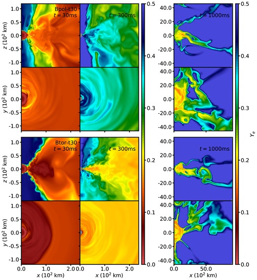
Same as Fig. 5, but for electron fraction.
3.2 Overview of post-collapse outflows
After we trigger the collapse of the HMNS, the system then resembles a BH–torus system. In all cases, there is an increase in outflow caused by a magnetized shock wave launched by the collapse of the HMNS, and a subsequent settling into steady accretion on to the newly formed BH. This effect shows up most prominently in the Btor-t30 model, where it is not masked by other outflows, and is noticeable as a spike in mass ejection at |$t\gtrsim 30\ \mathrm{ms}$| in Fig. 2. In the Bpol-t30 case, we find that expansion of the torus due to the action of the MRI causes |$\sim\!\! 10~{{ \rm per\, cent}}$| of the torus mass to not have enough angular momentum to maintain its orbit, plunging into the BH on a time-scale of ≲1 ms after collapse. For the Btor-t30 run, we find that only 1 per cent of material is caught in the collapse, in comparison. This is a result of disc spreading and accretion induced by the MRI taking longer to initiate, as well as comparatively weaker initial magnetically driven outflows, resulting in a much more compact torus configuration – the torus centroid is located only 1.1 times further out than its initial position, as opposed to the 2.2 times increase in the Bpol-t30 case. For the longer lived HMNS cases, Bpol-t100 and Btor-t100, the longer time for accretion and viscous spreading to occur causes even more mass to be lost upon collapse, |$\sim\!\! 25$| and |$\sim\!\! 15~{{ \rm per\, cent}}$|, respectively, of the torus is accreted instantaneously.
In all cases, material that is ejected by |$t \gtrsim 600\ \mathrm{ms}$| is very similar to that of previous BH–torus studies in (GR)MHD, and tends to be in stochastic, slow (v ≲ 0.1c) MRI turbulence driven outflows, with an electron fraction of Ye ∼ 0.2–0.3 set by the equilibrium value in the torus (see e.g. Siegel & Metzger 2018). The thermally driven outflows are noticeable as a peak in the velocity and electron fraction histograms in Fig. 3 at v ∼ 0.05c and Ye ∼ 0.2.
The total mass ejected asymptotes to similar values at times t ∼ 1 s in both Bpol-t30 and Btor-t30, although a significantly larger fraction (factor 2, in comparison) of that mass is contained in redder, slower outflows in Btor-t30. While the average electron fraction remains the same in the blue outflows between the two runs, they too tend to be about half as fast in the toroidal model.
Both Bpol-t100 and Btor-t100 are very similar to their |$30\ \mathrm{ms}$| counterparts. Although they are run for a shorter amount of simulation time (|$t \sim 0.5\ \mathrm{s}$|), cumulative mass ejection and mass ejection rates match those from their counterparts well at that time, and we do not expect large differences in the thermally driven outflows past this point in time. This is explained by mass ejection being dominated by MHD stresses in the torus at early times (|$t \lesssim 100\ \mathrm{ms}$|) and thermal outflows at late times (|$t \gtrsim 400\ \mathrm{ms}$|), the latter being mostly unaffected by the lifetime of the HMNS. The neutrino-driven winds between 30 and 70 ms tend to be diminished by the accretion flow on to the HMNS, which cools more effectively than the neutrino irradiation heats it, making ejecta in this time from lower density, lower temperature edges of the flow where neutrino heating dominates. While total outflows remain the same, the proportion of blue outflows when compared at the latest common time (|$t=0.5\ \mathrm{ s}$|) is 5 per cent higher for the longer lived HMNS models, and they tend to be concentrated in magnetically driven and neutrino-driven winds with velocities v ∼ 0.3–0.5c.
3.3 Tracer particles and nucleosynthesis
The r-process abundance patterns at t = 30 yr for all of our simulations are shown in Fig. 7. All models broadly follow the solar r-process abundance pattern. Both increasing the HMNS lifetime and initializing with a toroidal field geometry result in less mass ejection on time-scales shorter than those required for weak interactions to raise the electron fraction above the critical value of Ye ≳ 0.25. As a result of this, we see a drop in abundances with A > 130 in these models compared to the Bpol-t30 model, qualitatively consistent with other studies.
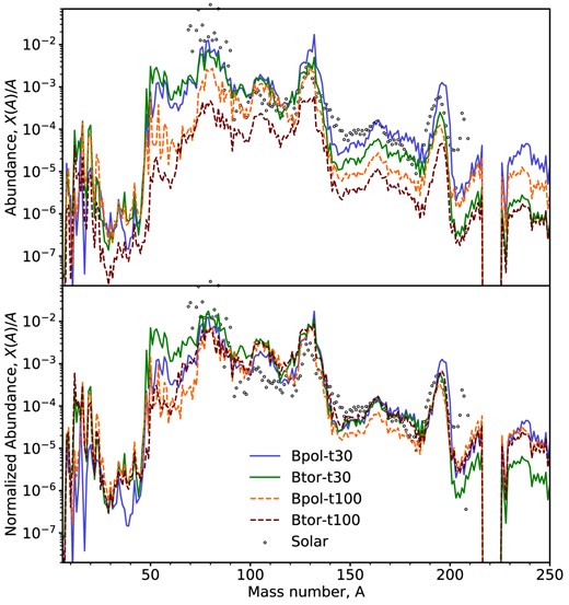
Top: Abundances at 30 yr computed with the nucleosynthesis code skynet using the trajectories of all unbound tracer particles past 1000 km in the simulation. Shown in open circles are the solar r-process abundances from Goriely (1999), scaled such that the abundance at the second peak (A = 130) matches that of our Bpol-t30 model. Bottom: Same as top, except that all models are scaled such that they match the abundances of Bpol-t30 at A = 130, to illustrate differences in abundance pattern assuming that the ejected mass is the same.
The lifetime of the HMNS has the largest impact on the abundance distribution, with a decrease of almost 100 times from model Bpol-t30 to Bpol-t100 in these elements. However, the significant decrease in initially purely magnetic-driven outflows (e.g. between Bpol-t30 and Btor-t30) also causes a drop by almost half an order of magnitude. This is consistent with the expectations from the distribution of our particles in |$s_\mathrm{k_B}-Y_\mathrm{ e}-v$| space.
Overall, we find that all four models produce the three process peaks. By normalizing all the abundance patterns to the second peak of Bpol-t30, we find that the relative ratios of light to heavy r-process elements are very similar between models. The Bpol-t100 model tends to underproduce the rare-earth peak, which could be due to the increased high-entropy (s ≳ 100kB per baryon) neutrino-driven winds during |$30\ \mathrm{ms}\le t \le 100\ \mathrm{ms}$| that makes lighter seed nuclei for the r-process to build on (Lippuner & Roberts 2015). We speculate that if more thermally driven outflows with lower entropy and Ye ∼ 0.3 were captured by running the simulation longer, this discrepancy may vanish as the fraction of ejecta from neutrino-driven winds decreases. We also see a relative underproduction of actinides and overproduction of lighter (A ≲ 100) r-process elements in Btor-t30. This is consistent with the additional high Ye material ejected during HMNS collapse, which makes a substantial contribution to the total ejected mass.
4 COMPARISON TO PREVIOUS WORK
4.1 3D simulations
Kiuchi et al. (2023) carry out simulations in full GRMHD of a magnetized NS–NS merger, including neutrino leakage and absorption, and using the SFHO EOS. They run the simulation until |$\sim\!\! 1.1\ \mathrm{s}$| post-merger, with the HMNS surviving for 17 ms, and report mostly red post-merger outflows with broad range of electron fractions peaking at Ye ∼ 0.24 and travelling at v ≲ 0.15c. The material with Ye ≳ 0.25 is ejected via turbulent angular momentum transport from MRI operating in the disc after HMNS collapse, which travels too slow to power the blue kilonova from GW170817, consistent with other MHD simulations of BH–torus ejecta (Fahlman & Fernández 2022; Hayashi et al. 2022; Curtis et al. 2023b). They note a lack of magnetic ‘tower’ structure that drives outflows in the polar regions. Our Btor-t30 model most closely matches the post-merger state found in their work, and our outflows show broad agreement in the electron fraction and entropies of the ejecta, as well as a lack of ‘tower’ outflows. We do not, however, find a sharp cut-off in post-merger mass ejection with velocities v > 0.15c, but rather a gradual fall-off. This could be due to the increased lifetime of our HMNS, as well as the lack of special relativistic effects limiting the velocity of our outflows.
The simulations of Combi & Siegel (2023a) are also of a GRMHD NS binary with neutrino leakage and absorption, using the APR EOS. Their HMNS survives |$\sim\!\! 60\ \mathrm{ms}$| (the duration of the simulation), and ejects |$\sim\!\! 10^{-2}\ \mathrm{ M}_\odot$| of ejecta, travelling with v ≳ 0.1c mainly through disc winds. Through irradiation from the HMNS, the vast majority of this ejecta has 〈Ye〉 ∼ 0.3. In our poloidal set-ups, we also find sustained mass ejection rates of |$\sim\!\! 0.1\ \mathrm{ M}_\odot \, \mathrm{ s}^{-1}$|. They find that about 5 per cent of their outflows are generated from HMNS magnetized ‘tower’ outflows, consistent with our simulations where we find that only |$\sim\!\! 10^{-4}\ \mathrm{ M}_\odot$| (|$\sim\!\! 1~{{ \rm per\, cent}}$|) come from magnetized outflows from the HMNS. They also find similar amounts of matter, |$\sim\!\! 10^{-3}\ \mathrm{ M}_\odot$|, moving with v > 0.25c and Ye > 0.25, which is consistent with our simulations.
Interestingly, they find that this result is consistent with the early blue kilonova of GW170817 through a simple kilonova model (Combi & Siegel 2023b). This is consistent with the recent kilonova models of Bulla (2023) and Ristic et al. (2023), which show that massive (|$\sim\!\! 10^{-2}\ \mathrm{ M}_\odot$|), blue (Ye > 0.25), disc winds with v ∼ 0.05c are sufficient to power the early blue kilonova at times ≲5 d. This suggests that our very similar outflows would also be able to power the blue kilonova, although this cannot be confirmed without self-consistent modelling.
de Haas et al. (2022) examine the effects of magnetic field strength and geometry within the HMNS on the outflows mapped from a post-merger system, using 3D GRMHD neutrino leakage/absorption simulations with the LS220 EOS. They find that a magnetar strength poloidal magnetic field in the HMNS (|$B\sim 10^{15}\ \mathrm{G}$|) is capable of ejecting |$\sim\!\! 10^{-3}\ \mathrm{ M}_\odot$| of ejecta travelling with a wide range of velocities, 0.05c < v < 0.6c, and Ye ≳ 0.25. They find that decreasing the field strength by an order of magnitude decreases the ejecta to |$\sim\!\! 10^{-4}\ \mathrm{ M}_\odot$|, while also lowering the maximum velocity of the ejecta to ∼0.2c. In addition, they show that changes in the imposed field geometry have similar effects. We find similar distributions of ejecta in velocity and electron fraction in our simulations, with mass ejection rates similar in our poloidal runs, despite in our simulations imposing a weaker (|$10^{14}\ \mathrm{G}$|) initially toroidal field within the HMNS, but this changes quickly |$(\lesssim\!\! 20\ \mathrm{ms}$|) through the dynamics inside the HMNS. The field acquires a large poloidal component that peaks at values of |$3\times 10^{16}\ \mathrm{G}$|, and in the case of the 100 ms HMNS saturates at |$8\times 10^{16}\, \mathrm{G}$|. Additionally, they find changing magnetic field geometry to be primed for more stress-driven outflow results in less A > 130 element nucleosynthesis, consistent with our findings.
Curtis et al. (2023a) and Mösta et al. (2020) perform 3D GRMHD simulations using a two-moment (M1) and neutrino leakage scheme, respectively, the LS220 EOS, and the same HMNS remnant that survives for 12 ms after mapping in from a hydrodynamic merger simulation at 17 ms post-merger with an added |$B\sim 10^{15}\ \mathrm{G}$| poloidal field. Both studies find |$\sim\!\! 3\times 10^{-3}\ \mathrm{ M}_\odot$| worth of material ejected and velocities peaking at 0.15c, with a significant tail up to 0.5c. They highlight the difference in using an M1 versus leakage scheme for handling neutrinos, as the more advanced M1 scheme shifts the peak electron fraction of the ejecta up from distribution around Ye ∼ 0.25 to one peaking at Ye ∼ 0.35–0.45. Our results are similar in both velocity and electron fraction to the outflows from their system, especially to the leakage results of Mösta et al. (2020), with a mass ejection rate very similar to that of our Bpol-t30 and Bpol-t100 models.
4.2 2D simulations
Studies that use axisymmetric simulations find that neutrino-driven winds from the HMNS can reach velocities of v ∼ 0.15c, although the exact velocity, ejecta mass, and composition depend on the lifetime of the HMNS, prescription used for neutrino radiation, and the handling of angular momentum transport. Higher velocities are possible, but they come with increased irradiation of the ejecta, making a simultaneous match to the blue and red kilonovae difficult (e.g. Lippuner et al. 2017; Fahlman & Fernández 2018; Nedora et al. 2021; Fujibayashi et al. 2023).
However, the recent hydrodynamic simulations of Just et al. (2023), mapped in from a merger simulation, include a more advanced energy-dependent neutrino leakage scheme and utilize the SFHO EOS, as well as varying remnant survival times in pseudo-Newtonian potential. They find neutrino-driven winds with a mass of |$\sim\!\! 10^{-2}\ \mathrm{ M}_\odot$| and velocity 〈vej〉 ∼ 0.2c for their remnants that survive for a comparable amount of time, |$\sim\!\! 100\ \mathrm{ms}$|. The mass ejection rates are broadly similar to our simulations, |$\sim\!\! 10^{-2}\ \mathrm{ to} \ 10^{-1}\ \mathrm{ M}_\odot \, \mathrm{s}^{-1}$|, and due to the ejection mechanism, these tend to be high electron fraction Ye > 0.25. They produce few elements with A > 130, most consistent with our Btor-t100 run, which in our case produces the most dominant neutrino-driven wind.
In addition, Shibata et al. (2021a) perform unique 2D resistive GRMHD simulations, with a mean field prescription to prevent the damping of the magnetic dynamo in axisymmetry. Their simulations start from prescribing a toroidal magnetic field on to the outcome of a GRHD merger simulation using the DD2 EOS, similar to our idealized initial conditions. The set-ups of their low-resistivity simulations are most comparable to our ideal MHD treatment, although their remnant has a different rotational profile, and survives for the duration of the simulation. They find ejecta masses of |$\sim\!\! 0.1\ \mathrm{ M}_\odot$| that plateau at |$\sim\!\! 500\ \mathrm{ms}$|, with average velocities of 0.5c. The velocity and electron fraction of the ejecta are comparable to those of our Btor-t30 run, although we find more low electron fraction ejecta and less mass ejected, by an order of magnitude.
4.3 Discussion
In general, our results are in agreement with those of the literature. They tend to span a broader range of electron fraction than that found by other studies in the literature, in particular with a larger component of material ejected with Ye < 0.2. We speculate that this is due to the simplicity of our leakage scheme in comparison to the more advanced energy-dependent leakage, M1, or Markov Chain Monte Carlo (MCMC) schemes (see Appendix A) in combination with the idealized initial conditions for the torus, which tends to eject material in fast, magnetic stress-driven outflows that can escape neutrino interactions.
Our HMNS itself has a lower mass ejection rate than others found in the literature. This is also likely partially due to the neutrino scheme, which yields less efficient heating of matter surrounding the HMNS, with implications for the neutrino-driven winds. Additionally, the importance of the magnetic field configuration and resolution within and around the HMNS likely plays a large role. Our toroidal field embedded in the HMNS ejects mass similar to that of Kiuchi et al. (2023), but ejects an order of magnitude less mass than poloidal field configurations (e.g. de Haas et al. 2022; Combi & Siegel 2023a; Curtis et al. 2023a). We do not resolve the most unstable wavelength of the MRI inside our HMNS, meaning that MRI-driven ejection is not captured. Finally, we note that changing the rotation profile of the HMNS to match those of merger simulations could result in additional mechanical oscillation-powered outflows as angular momentum is transported in the HMNS.
5 CONCLUSIONS
We have performed |$\sim\!\! 1\ \mathrm{s}$| long 3D MHD simulations of an idealized post-merger system consisting of a 2.65 M⊙ HMNS and |$0.1\ \mathrm{ M}_\odot$| torus. We utilize Newtonian self-gravity, the hot APR EOS, a leakage/absorption scheme to handle neutrino interactions, and a pseudo-Newtonian potential after BH formation. Motivated by the sensitivity of the HMNS collapse time to physical processes, and necessitated by our use of Newtonian gravity, we use two parametrized HMNS collapse times of 30 and 100 ms to determine the effects of an HMNS as a central remnant. To evaluate the effects of the initial magnetic field geometry, we utilize either a toroidal or poloidal magnetic field threaded through the torus.
The outflows are similar to those produced by idealized BH–disc set-ups, with a broad distribution of electron fraction and velocities. The HMNS itself tends to drive additional fast (v ≳ 0.2c) high electron fraction outflow (Ye > 0.3) from the torus while it survives, due to oscillations in the remnant and energy from neutrino irradiation. Upon collapse, accretion on to the BH drives additional outflows, and slower (v < 0.1c), redder (Ye ∼ 0.2) MRI-driven outflows begin to dominate the total mass ejection.
We find that in all cases, a shock wave is launched upon collapse of the HMNS as the torus and newly formed BH settle into an accreting state. The creation of a rarefaction wave has been seen in previous 2D hydrodynamic simulations (Fahlman & Fernández 2018), but in the magnetized 3D case we find that it drives significant outflows, especially noticeable in the short-lived HMNS. The launching of a magnetized shock by supramassive NS collapse has been explored in baryon-free environments in the context of powering fast radio bursts (the ‘blitzar’ mechanism; Most, Nathanail & Rezzolla 2018), but it is unknown whether this shock would drive mass outflows in a baryon-polluted system. Whether this effect is due to our instantaneous collapse in Newtonian gravity, idealized initial conditions, or is a real effect, remains to be seen.
Neutrino-driven winds from a longer lived (|$t \gt 30\ \mathrm{ms}$|) HMNS tend to be suppressed by the accretion of matter on to the HMNS, which cools efficiently. Due to accretion from the torus and oscillations of the HMNS, we find a lack of high-velocity ‘tower’ ejecta from the polar regions, which tend to be too dense to eject large amounts of matter moving at relativistic velocities.
Nucleosynthesis in the outflows tends to predict a robust r-process up to the second peak (A ∼ 130), with order of magnitude variations past A ∼ 130 caused by changing HMNS lifetime or magnetic field geometries.
Across all models, we find M ∼ 10−3 M⊙ of ejecta with Ye > 0.25 and v > 0.25c. Whether or not this can completely account for the blue kilonova of GW170817 is model-dependent, as simple two-component models require an order of magnitude more blue, fast ejecta. However, multidimensional models with more realistic opacities, thermalization, heating rates, and viewing angle dependence find that a massive (|$10^{-2} \ \mathrm{ M}_\odot$|), slower (v ∼ 0.1c) wind is all that is required. If the latter is the case, then our outflows are in principle capable of powering the blue kilonova.
The main limitations of our simulations are the use of an approximate neutrino scheme and Newtonian gravity. In testing of our neutrino scheme (see Appendix A), we find results similar to those of other leakage comparisons, with an underprediction of neutrino heating resulting in slower, lower Ye outflows as compared to more robust Monte Carlo (MC) or M1 schemes (e.g. Ardevol-Pulpillo et al. 2019; Radice et al. 2022; Curtis et al. 2023a). For a similar mass HMNS in GR, we estimate that the HMNS could be up to 1.5 times as compact as our Newtonian HMNS upon merger. This reduces the amount of neutrino emission in the Newtonian HMNS compared to a general relativistic one, and results in the same underpredictions of neutrino absorption in the torus, an effect that has been documented in the context of core-collapse supernova simulations (e.g. Liebendörfer et al. 2001; Marek et al. 2006; Müller, Janka & Marek 2012; O’Connor & Couch 2018; Mezzacappa 2023). In addition, although we find a lower density magnetized funnel in our simulations, it is unlikely that we are able to correctly model jet formation in our simulations. Inclusion of special relativistic effects in the MHD equations results in corrections that are of the order of ∼v/c, so we estimate uncertainties in the fast tail of our ejecta of |$\sim\!\! 50~{{ \rm per\, cent}}$|, but the majority of outflows sit at v < 0.1c, which results in a 10 per cent inherent uncertainty.
Acknowledgement
We thank Coleman Dean and Suhasini S. Rao for helpful suggestions and discussions. SF and RF were supported by the Natural Sciences and Engineering Research Council of Canada (NSERC) through Discovery Grant RGPIN-2022-03463, and SM by NSERC Discovery Grant RGPIN-2019-06077. The software used in this work was in part developed by the U.S. Department of Energy (DOE) NNSA-ASC OASCR Flash Center at the University of Chicago. Data visualization was done in part using VisIt (Childs et al. 2012), which is supported by DOE with funding from the Advanced Simulation and Computing Program and the Scientific Discovery through Advanced Computing Program. This research was enabled in part by support provided by WestGrid (www.westgrid.ca), the Shared Hierarchical Academic Research Computing Network (SHARCNET; www.sharcnet.ca), Calcul Québec (www.calculquebec.ca), and Compute Canada (www.computecanada.ca). Computations were performed on the Niagara supercomputer at the SciNet High Perfomance Computing (HPC) Consortium (Loken et al. 2010; Ponce et al. 2019). SciNet is funded by the Canada Foundation for Innovation, the Government of Ontario (Ontario Research Fund – Research Excellence), and by the University of Toronto.
DATA AVAILABILITY
The data underlying this article will be shared on reasonable request to the corresponding author.
References
APPENDIX A: HMNS NEUTRINO LEAKAGE SCHEME
In this appendix, we detail the implementation of additions to our neutrino scheme to include the effects of HMNS irradiation in the domain, in particular the effects of neutrino heating on the torus. Full details of the scheme are outlined in Fahlman & Fernández (2022). The end goal of the implementation is scheme accurate to within an order of magnitude with limited computational costs. It is well known that neutrino leakage schemes tend to underpredict the lepton number change and energetics in merger simulations (e.g. Foucart et al. 2020; Radice et al. 2022; Curtis et al. 2023a), and as such we do not attempt to create a totally quantitatively accurate scheme.
A1 Neutrino implementation
The HMNS is a source of neutrino emission, so we change our lightbulb-leakage scheme to have an additional component of heating from the HMNS applied to the domain. We extend the implementation of Metzger & Fernández (2014) and Lippuner et al. (2017) for heating fluid elements outside the neutrinosphere, which requires the location of the neutrinosphere, as well as the temperature and luminosity of the neutrino emission.
The explicit heating and cooling terms are given in the appendices of Fernández & Metzger (2013) and Metzger & Fernández (2014). What requires modification is the total neutrino luminosity input from the HMNS, which is then normalized by the blackbody radiation of the neutrinos at the neutrinosphere, and a radial component to account for the flux hitting the cell,
In previous simulations, the neutrino luminosity |$L_{\nu _i}$|, neutrinosphere temperature, |$T_{ns,{\nu _i}}$|, and neutrinosphere radius Rns,ν were user defined parameters, and we now make them self-consistent. We find the total luminosity of the HMNS by summing up the individual emissivities of each cell within the HMNS. The neutrinosphere radius is not assumed to be spherically symmetric, and is allowed to change with θ and ϕ. It is determined as the first location radially outwards at which the optical depth is less than or equal to 2/3,
The radial optical depth for each species is calculated along each direction using the numerical summation |$\tau _{\nu _i}= \sum \kappa _{\nu _i}(r) \mathrm{d}r$|, where we utilize the analytical expressions for κ from Ruffert, Janka & Schaefer (1996), which include the effects of energy-averaged scattering and absorption processes on to neutrons and protons. The neutrino temperature is then determined from the average neutrino energy in the neutrinosphere:
where |$Q_{\nu _i}^\mathrm{eff}$| and |$R_{\nu _i}^\mathrm{eff}$| are the effective energy and lepton number change for each neutrino species, the explicit forms for which are defined in Fernández et al. (2019a), equations (3) and (4). The factors of the Fermi integrals, |$\mathcal {F}_n(0)$|, come from expanding the explicit forms of |$Q^\mathrm{eff}_{\nu _i}$| and |$R^\mathrm{eff}_{\nu _i}$|.
The neutrino radiation is then further attenuated by a factor of |$\mathrm{e}^{-2\tau _{\nu _i}}$|, where |$\tau _{\nu _i}$| is the radially integrated optical depth along the line of sight from the cell to the HMNS.
Within the neutrinosphere, the irradiation is identical, except that it relies on the spherically symmetric enclosed luminosity and temperature at each radial cell. These enclosed quantities are then used in equations (A1), (A2), and (A3) to calculate the normalized luminosity used in the heating and lepton number change rates. In practice, however, the luminosity within the HMNS is dampened to negligible rates by the exponential of the massive opacities (|$\tau _{\nu _i}\sim 10^4$|), which drops steeply across one single cell at the HMNS neutrinosphere with our current resolution.
Additionally, we improve the lightbulb scheme for emission from the torus by integrating |$\tau _{\nu _i}$| for absorption from neutrinos emitted by the torus. While this is a subdominant effect compared to both cooling from the torus and irradiation from the HMNS, the previous scheme of Fahlman & Fernández (2022) has problems with high-density tori, especially after they experience shocks from the HMNS oscillation. These shocks can artificially increase |$\tau _{\nu _i}$| in the outer regions of the torus, as the previous scheme used the value of |$\tau _{\nu _i}$| at the density maximum for the luminosity reduction in the entire torus.
We develop a simple new scheme that relies on integration of |$\tau _{\nu _i}$| in the radial and polar directions. First, we determine the four optical depths shown in Fig. A1. The first is along the radial line of sight from the emission maximum to each point (τ1), the radial optical depth along the equator to the radius at which the point lies (τ2), the angular optical depth from the torus equator to the emission maximum (τ3), and to the point (τ4). The optical depth is then taken to be the maximum of the two possible path lengths,
to avoid issues with points around the HMNS where one of the paths can have unphysically small optical depths. This is similar to other neutrino leakage schemes (e.g. Ruffert et al. 1996; Neilsen et al. 2014; Siegel & Metzger 2018; Werneck et al. 2023).
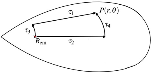
Integrated line-of-sight optical depths used in determining the reduction in self-irradiation heating from torus emission. The torus is taken to be a lightbulb that emits from two points slightly above and below the mid-plane at a radius Rrm, to each point in the domain, P(r, θ).
We compare snapshots of the net energy and lepton number change source terms from our scheme to the time-stationary MC neutrino transport code sedonugr (Richers et al. 2015, 2017) in Figs A2 and A3. sedonugr utilizes an MC algorithm accounting for emission, absorption, and scattering of neutrinos for a given fluid background and EOS to return the local energy and lepton number change rates for a fluid parcel. MC schemes are among the most accurate in the literature (e.g. Richers et al. 2015, 2017; Ryan, Dolence & Gammie 2015; Miller et al. 2019; Foucart et al. 2020), so the source terms returned by sedonugr are a good benchmark that we can compare our more approximate lightbulb-leakage scheme to. Snapshots from 2D slices of our spherical domain at t = 0, 1, and 30 ms are taken as comparison points. The effects of neutrinos start to become negligible due to decreased emission and increased transparency as the torus dissipates, and for this reason, we focus our comparison at earlier time-steps, with earlier agreement being much more impactful.
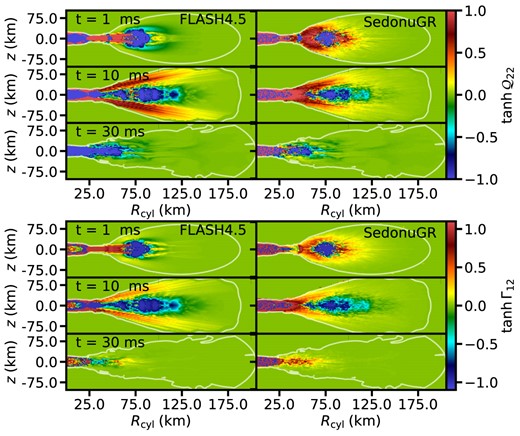
Comparison of neutrino source terms for a 0.1 M⊙ torus and 2.65 M⊙ HMNS at t = 0, 1, and 30 ms in flash4.5 (left) to sedonugr (right). The top six panels compare rate of energy change per unit mass, and the bottom six panels show rate of lepton number change per baryon. The background fluid snapshots are taken as 2D slices at ϕ = 0 from the flash4.5 domain at the specified time, with the |$10^9 \ \mathrm{g\, cm}^{-3}$| white contours delimiting the approximate edge of the torus, where the neutrino source terms are set to 0. The lightbulb-leakage scheme tends to underestimate the heating and lepton change at all times, leading to less energetic, lower Ye neutrino-driven outflows than those in an MC scheme.
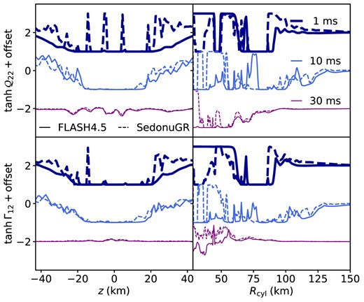
Comparison of neutrino source terms for a 0.1 M⊙ torus and 2.65 M⊙ HMNS at t = 0, 1, and 30 ms in (top) rate of energy change per unit mass, and (bottom) rate of lepton number change per baryon. The absolute values of the source terms for t = 1 and 30 ms have been offset by a constant (±2) for each time for visual clarity. The background fluid snapshots are from the flash4.5 domain at the specified time. Left: Vertical slices at ϕ = 0 and r = rcirc (through the torus density maximum). Right: Radial slices at ϕ = 0 and θ = 90 (through the equator). The neutrino source terms from flash4.5 are shown as solid lines, while the source terms from sedonugr as dashed lines. Changing colour and line thickness denote different time snapshots.
The neutrino scheme recreates the overall energy and lepton number change rates to within a factor of a few, following a similar spatial distribution. As the scheme progresses, cooling of material is overestimated by an order of magnitude, especially in the mid-plane of the torus and close to the HMNS. We show this both with 2D colourmaps, as well as a numerical comparison of the schemes by taking a radial slice through the domain at the equator, and a vertical slice at the density maximum of the torus. While it is difficult to extrapolate the effects of the discrepancies on our outflows, we can speculate that increased cooling near the mid-plane of the HMNS may result in less neutron-rich material being ejected by magnetically driven outflows, which is also found by Curtis et al. (2023a) in their leakage scheme comparison. However, the majority of matter affected is also likely to be accreted upon HMNS collapse, as its small angular momentum causes it to circularize at a radius smaller than the ISCO upon collapse to BH.
