


ABSTRACT
The effect of dust attenuation on a galaxy’s light depends on a number of physical properties, such as geometry and dust composition, both of which can vary across the faces of galaxies. To investigate this variation, we continue analysis on star-forming regions in 29 galaxies studied previously. We analyse these regions using Swift/UV Optical Telescope and Wide-field Infrared Survey Explorer images, as well as Sloan Digital Sky Survey/Mapping Nearby Galaxies at Apache Point Observatory emission line maps to constrain the relationship between the infrared excess (IRX) and the ultraviolet spectral index, β, for each star-forming region. This relationship can be used to constrain which dust attenuation law is appropriate for the region. We find that the value of Dn(4000) for a region is correlated with both IRX and β, and that the gas-phase metallicity is strongly correlated with the IRX. This correlation between metallicity and IRX suggests that regardless of aperture, metal-rich regions have steeper attenuation curves. We also find that integrated galactic light follows nearly the same IRX–β relationship as that found for kpc-sized star-forming regions. This similarity may suggest that the attenuation law followed by the galaxy is essentially the same as that followed by the regions, although the relatively large size of our star-forming regions complicates this interpretation because optical opacity and attenuation curves have been observed to vary within individual galaxies.
1 INTRODUCTION
The accurate determination of galactic star formation rates (SFRs) is crucial in the study of galaxy evolution. Rest frame near ultraviolet (UV) emission is one of the most common tracers of recent star formation (Kennicutt & Evans 2012). This is especially true at high redshift where rest-frame UV is more easily accessible than rest-frame infrared (IR). Observations of star formation are often complicated by the production of dust, which hides newly formed stars. In fact, it has been shown that the fraction of star formation hidden by dust is dominant at redshifts z ∼ 1–3 (Le Floc’h et al. 2005; Magnelli et al. 2011; Reddy et al. 2012). Furthermore, UV light is preferentially extinguished by dust. Our ability to correct for the effect of dust depends heavily upon our knowledge of the appropriate extinction and attenuation laws. To learn how to correct for these effects, we often rely on nearby systems.
Attenuation laws attempt to quantify the effects that dust, of varying composition and geometrical configuration, has on the propagation of light (see Salim & Narayanan 2020, for a review). They differ from extinction laws in that they account for the geometrical complexities that exist in physical systems. They are generally parametrized using the same two basic properties (Noll et al. 2009). The first is the general shape of the curve as a function of wavelength. The second is the strength of the excess attenuation at 2175 Å, referred to as the 2175 Å bump. Both correlate with the intrinsic physical properties of the object being observed, such as the SFR and total stellar mass (Calzetti et al. 2000; Wild et al. 2011; Salim, Boquien & Lee 2018), as well as dust composition, geometry, and the V-band attenuation (AV; e.g. Boquien et al. 2022).
The physical properties that affect the shape of the attenuation law can vary both from galaxy to galaxy as well as across a single galaxy (Calzetti et al. 2000; Charlot & Fall 2000; Wild et al. 2011). The fact that dust extinction laws within a galaxy vary greatly from sightline to sightline (e.g. Cardelli, Clayton & Mathis 1989; Fitzpatrick 1999; Gordon et al. 2003) means that the attenuation curve will also vary, further complicating the measurements of small-scale star formation (Hoversten et al. 2011; Hagen et al. 2017; Molina et al. 2020b; Zhou et al. 2022).
Although it is common to apply attenuation corrections when fitting spectral energy distributions (SEDs), such corrections become difficult when photometry is only available in a few bands. When these situations arise, corrections can be obtained by using a combination of attenuation-sensitive star formation tracers and the amount of emission in the IR. One such scheme involves the relationship between the UV spectral index, β, and the IR excess (IRX; Calzetti, Kinney & Storchi-Bergmann 1994; Meurer, Heckman & Calzetti 1999; Calzetti et al. 2000). This scheme requires assuming that all the light emitted by young stars in the UV that is attenuated by dust is then re-emitted in the IR, and that there is no sightline dependence on the UV attenuation (da Cunha, Charlot & Elbaz 2008). This relationship becomes especially useful at high redshift where rest-frame IR light becomes difficult to observe, and correction based solely on rest-frame UV light might be necessary.
The IRX is defined as IRX ≡ log(LTIR/LFUV), where LTIR refers to the total IR luminosity of the source, often measured between 3 and 1100 µm, and LFUV is the monochromatic luminosity at some far-UV (FUV) wavelength, often that of the Galaxy Evolution Explorer (GALEX) FUV filter (Meurer et al. 1999). The IRX thus provides a measure of the amount of light initially emitted in the UV that is absorbed and re-emitted by dust in the IR, and is, in effect, a good tracer of the attenuation.
The UV spectral index, β, quantifies the shape of the SED of a galaxy in the UV band by assuming that the stellar continuum is well approximated by Fλ ∝ λβ (Calzetti et al. 1994). The relationship means that negative values of β are characteristic of very young populations with little dust, and positive values of β correspond to older or dustier populations (see Calzetti 2013).
The relationship between IRX and β has been studied for both starburst (e.g. Meurer et al. 1999; Kong et al. 2004; Takeuchi et al. 2012; Nagaraj et al. 2021) and local star-forming galaxies (e.g. Dale et al. 2009; Takeuchi et al. 2012; Salim & Boquien 2019), as well as on sub-galactic scales across star-forming galaxies (e.g. Boquien et al. 2009, 2012). Meurer et al. (1999) first defined an IRX–β relationship for starburst galaxies. Later measurements of the relationship for more normal star-forming systems, however, found deviations from the Meurer et al. (1999) law. For example, Boquien et al. (2012) inspected seven, face-on, star-forming galaxies on a pixel-by-pixel basis and found that deviations from the Meurer et al. (1999) relationship could be caused either by variations in the intrinsic UV colour of the underlying stellar populations or by varying attenuation law slopes. Alternatively, Takeuchi et al. (2012), exploring the same deviation, found that the sample of starburst galaxies studied by Meurer et al. (1999) did, in fact, follow the same relationship found for normal star-forming galaxies, but that aperture effects played a large role in shifting the apparent IRX–β relationship.
While previous work has investigated relationships between the IRX and β on sub-galactic scales (Muñoz-Mateos et al. 2009; Boquien et al. 2012; Ye et al. 2016), those studies were limited by the number of galaxies with resolved regions. We attempt to understand and explain the drivers of attenuation in those regions, and the relationship between attenuation in resolved regions and attenuation in integrated galactic light in a larger sample of 29 galaxies. Our work is a continuation of that started by Molina et al. (2020b), which focused on the source of variation in the attenuation laws by using the optical and near-UV (NUV) tracers |$\tau ^l_{\rm B}$|, or Balmer optical depth, and β.
We combined data from the Swift/UV Optical Telescope (UVOT), the Mapping Nearby Galaxies at Apache Point Observatory (MaNGA) integrated field unit survey, and the Wide-field Infrared Survey Explorer (WISE) for 29 galaxies examined by Molina et al. (2020b) to study dust attenuation via the IRX–β relationship in resolved, kpc-sized star-forming regions. These galaxies were drawn from a larger catalogue, created to study star formation and its quenching in the local Universe (Molina et al. 2020a). We also compared the resulting relationship with that for the integrated galactic light, and examined the role of a number of physical parameters in driving the scatter of the relationship.
In Section 2, we introduce the sample. Section 3 describes the steps that were taken to process the data. We introduce the methodology behind defining and analysing the star-forming regions in Section 4. In Section 5, we investigate the effect that observed galaxy properties have on the relationship between IRX and β. We discuss and conclude upon our findings in Section 6. We assume a Lambda cold dark matter cosmology, with Ωm = 0.3, |$\Omega _\Lambda = 0.7$|, and H0 = 70 km s−1 Mpc−1.
2 SAMPLES AND DATA SET
2.1 Target selection
This work focuses on a subset of galaxies drawn from the larger Swift/MaNGA Value Added Catalogue (SwiM VAC; Molina et al. 2020a), created to study star formation and its quenching in nearby galaxies. The SwiM VAC consists of Swift/UVOT images, a wide variety of MaNGA emission line maps (including indices measured from MaNGA spectra), and Sloan Digital Sky Survey (SDSS) images. Molina et al. (2020b) used the catalogue to investigate the variation in attenuation laws for resolved, kpc-sized star-forming regions. They selected 29 of the original 150 SwiM VAC galaxies with appropriate SFRs and properties and used reddening-insensitive emission line ratios to identify galaxies where the majority of pixels were star forming according to the three standard emission line diagnostic diagrams, commonly referred to as the Baldwin, Phillips & Terlevich (1981, hereafter BPT) diagrams (Kauffmann et al. 2003; Kewley et al. 2006). Here, we further explore dust attenuation in those 29 galaxies. The basic properties of the sample galaxies can be found in Table 1. The galaxies have a median redshift of zm = 0.03, and have masses that span the range 8.8 ≤ log(M/M⊙) ≤ 10.7, similar to the sample used in Battisti, Calzetti & Chary (2016).
Basic properties of the sample of star-forming galaxies.
| Galaxy | Galaxy | SDSS | Rpet | log(M*) | log(SFR) | |||
|---|---|---|---|---|---|---|---|---|
| I.D. | name | class | z | E(B − V)G | b/a | (arcsec) | (M⊙) | (M⊙ yr−1) |
| (1) | (2) | (3) | (4) | (5) | (6) | (7) | (8) | (9) |
| 1 | UGC 11696 | SF | 0.017 | 0.101 | 0.52 | 19 | 8.76 | −1.23 |
| 2 | SDSS J170653.67+321010.1 | SF | 0.036 | 0.039 | 0.82 | 17 | 9.15 | −0.68 |
| 3 | WISE J162856.63+393634.1 | SF | 0.035 | 0.010 | 0.48 | 16 | 9.19 | −0.62 |
| 4 | 2MASS J04072365−0641117 | SF | 0.038 | 0.098 | 0.60 | 16 | 9.25 | −0.71 |
| 5 | 2MASX J11044509+4509238 | SF | 0.022 | 0.008 | 0.88 | 16 | 9.27 | −1.52 |
| 6 | 2MASS J14135887+4353350 | SB | 0.040 | 0.013 | 0.71 | 12 | 9.31 | −0.61 |
| 7 | KUG 1016+468 | SF | 0.024 | 0.013 | 0.45 | 19 | 9.32 | −0.87 |
| 8 | SDSS J030659.79−004841.5 | SF | 0.038 | 0.070 | 0.78 | 16 | 9.40 | −0.61 |
| 9 | 2MASS J14132780+4354501 | SF | 0.040 | 0.013 | 0.40 | 16 | 9.43 | −0.56 |
| 10 | SDSS J024112.93−005236.9 | SF | 0.038 | 0.034 | 0.56 | 19 | 9.44 | −1.07 |
| 11 | 2MASS J15004786+4836270 | SF | 0.037 | 0.020 | 0.54 | 14 | 9.50 | −0.54 |
| 12 | 2MASXi J0740537+400411 | N/A | 0.042 | 0.052 | 0.59 | 18 | 9.50 | 0.47 |
| 13 | KUG 0757+468 | SF | 0.019 | 0.065 | 0.53 | 19 | 9.52 | −0.03 |
| 14 | 2MASX J14403849+5328414 | SB | 0.038 | 0.011 | 0.80 | 15 | 9.55 | −0.12 |
| 15 | KUG 0254−004 | SF | 0.029 | 0.066 | 0.80 | 17 | 9.65 | 0.00 |
| 16 | 2MASX J07522873+4950192 | SF | 0.022 | 0.059 | 0.50 | 20 | 9.67 | −0.86 |
| 17 | KUG 0751+485 | SB | 0.022 | 0.035 | 0.71 | 15 | 9.71 | −0.46 |
| 18 | 2MFGC 8582 | SF | 0.025 | 0.014 | 0.33 | 18 | 9.73 | −0.23 |
| 19 | 2MASX J07595878+3153360 | SB | 0.045 | 0.048 | 0.57 | 16 | 9.78 | 0.08 |
| 20 | KUG 1121+239 | SF | 0.028 | 0.019 | 0.80 | 21 | 9.79 | −0.45 |
| 21 | WISE J163226.31+393104.0 | SF | 0.029 | 0.009 | 0.87 | 17 | 10.0 | −0.53 |
| 22 | 2MASX J09115605+2753575 | SB | 0.047 | 0.028 | 0.48 | 15 | 10.1 | 0.17 |
| 23 | KUG 1343+270 | SF | 0.030 | 0.017 | 0.54 | 22 | 10.1 | −0.22 |
| 24 | 2MASX J11532094+5220438 | SF | 0.049 | 0.029 | 0.87 | 16 | 10.1 | 0.00 |
| 25 | KUG 1626+402 | SF | 0.026 | 0.009 | 0.70 | 20 | 10.2 | 0.15 |
| 26 | NGC 3191 | SF | 0.031 | 0.011 | 0.86 | 22 | 10.3 | 0.73 |
| 27 | LCSB S1611P | Galaxy | 0.056 | 0.010 | 0.40 | 16 | 10.4 | −0.13 |
| 28 | 2MASX J07333599+4556364 | SF | 0.077 | 0.091 | 0.89 | 17 | 10.5 | 0.94 |
| 29 | 2MASX J03065213−0053469 | SF | 0.084 | 0.070 | 0.88 | 17 | 10.7 | 0.56 |
Notes. Column 1: Galaxy I.D. number in this sample. Column 2: Galaxy name. Column 3: Galaxy class from Bolton et al. (2012); SF stands for star forming and SB stands for starburst. Column 4: Redshift from the NASA Sloan Atlas (Blanton et al. 2017). Column 5: Foreground extinction measurements for each galaxy from Schlegel, Finkbeiner & Davis (1998). Column 6: Ratio of minor axis to major axis from the NASA Sloan Atlas (Blanton et al. 2017). Column 7: Petrosian radii are calculated in the W3 band following the procedure outlined in Section 3.2. Column 8: Stellar masses are taken from SED fits from the MaNGA data reduction pipeline (Law et al. 2016). Column 9: SFRs using the H α luminosity are from the MaNGA data analysis pipeline (Westfall et al. 2019).
Galaxy I.D. 26 (NGC 3191) from the original sample of Molina et al. (2020b) is excluded from most of our analyses, as the Swift/UVOT imaging of the galaxy coincided with the appearance of a Type I superluminous supernova in its central parts (see Bose et al. 2018). Since observations in the other bands were not contemporaneous, comparisons between the MaNGA emission line maps, Swift UV observations, and WISE images cannot be used to produce a reliable value of β.
2.2 SDSS-IV/MaNGA and Swift/UVOT
Molina et al. (2020a) constructed the SwiM VAC by matching galaxies in the first data release of MaNGA fully reduced spectra from the data reduction pipeline (DRP; Bundy et al. 2015; Law et al. 2016; Yan et al. 2016b; Aguado et al. 2019) to Swift/UVOT observations. MaNGA is one of the three major surveys in SDSS-IV (Blanton et al. 2017), and utilizes hexagonal bundles of 2 arcsec fibres that are mounted directly on the Sloan 2.5 m telescope (Gunn et al. 2006) and are fed into the Baryon Oscillation Spectroscopic Survey spectrographs (Smee et al. 2013; Drory et al. 2015). The MaNGA survey aimed to target ∼|$10\, 000$| galaxies with uniform spatial coverage and a uniform distribution in stellar mass for M* > 109 M⊙, while also maximizing spatial resolution and signal-to-noise ratio (S/N) for each galaxy (Wake et al. 2017). The effective point spread function (PSF) of the resulting maps has a full width at half maximum (FWHM) of 2.5 arcsec (Law et al. 2015, 2016). MaNGA spectra have a resolving power R ∼ 2000, and cover a wavelength range 3622–10 354 Å, which provides many nebular diagnostic lines (Belfiore et al. 2019; Westfall et al. 2019). MaNGA spectra also have very small errors in their flux calibration (Yan et al. 2016a).
The Swift/UVOT is a 30 cm telescope with an effective plate scale of 1 arcsec pixel−1 (Roming et al. 2005). Here, we use the uvw2 and uvw1 images, which have PSF FWHM values of 2.92 and 2.37 arcsec, respectively. Notably, these FWHM values are similar to those of MaNGA. The basic properties of the two NUV filters are listed in Table 2. Each of the star-forming galaxies in our sample has a minimum S/N of 15 in both NUV filters for the integrated galaxy light, and our sample galaxies have median exposure times of 2296 and 2375 s in the uvw1 and uvw2 filters, respectively (Molina et al. 2020a).
Basic properties of the Swift UVOT uvw1 and uvw2 filters, and the WISE W3 filter.
| Central | PSF | Pixel | |
|---|---|---|---|
| Filter | wavelength | FWHM | size |
| (1) | (2) | (3) | (4) |
| uvw2 | 1928 Å | 2.92 arcsec | 1 arcsec |
| uvw1 | 2600 Å | 2.37 arcsec | 1 arcsec |
| W3 | 12 µm | 6.5 arcsec | 2.75 arcsec |
| Central | PSF | Pixel | |
|---|---|---|---|
| Filter | wavelength | FWHM | size |
| (1) | (2) | (3) | (4) |
| uvw2 | 1928 Å | 2.92 arcsec | 1 arcsec |
| uvw1 | 2600 Å | 2.37 arcsec | 1 arcsec |
| W3 | 12 µm | 6.5 arcsec | 2.75 arcsec |
Notes. Column 1: The filter. Column 2: The central wavelength of the filter. Column 3: The FWHM of the PSF for each filter. Column 4: The pixel size for each filter.
2.3 WISE
We supplement the above data set with IR images for the 29 galaxies from WISE. The WISE telescope, which has a 40 cm primary mirror, mapped the sky in four IR bands, with filters centred at 3.4, 4.6, 12, and 22 µm (Wright et al. 2010). The W1, W2, and W3 bands each have a PSF FWHM of about 6 arcsec, whereas the W4-band PSF FWHM is about 12 arcsec. The W1, W2, and W3 images also have angular pixel sizes of 2.75 arcsec, while the W4 images have a pixel size of 5.5 arcsec.
While the 22 µm W4 band is better suited in wavelength for probing the total IR luminosity of galaxies, it cannot resolve the kpc-sized star-forming regions of interest to this study. For this reason, we do not use W4 band photometry, and instead rely on W3 measurements.
3 DATA PROCESSING
3.1 Swift/UVOT data processing
We used Swift/UVOT count and exposure maps that were pre-processed by Molina et al. (2020b) with the Swift/UVOT pipeline1 (see section 3.2 of that paper). These count and exposure rates were further processed and presented in Molina et al. (2020a). We created images that were then corrected for the foreground extinction of each galaxy using the average total-to-selective extinction values for uvw1 and uvw2 found by Molina et al. (2020b). E(B − V) values were taken from Schlegel et al. (1998). We then applied the Fitzpatrick extinction law (Fitzpatrick 1999), chosen by Molina et al. (2020b) in order to facilitate comparison of their results with Battisti et al. (2016). E(B − V) values for each galaxy can be found in Table 1.
3.2 Sky subtraction
We followed the same procedure for subtracting the background from UVOT images as Molina et al. (2020b). To summarize, we first calculated the Petrosian radius of each galaxy in the uvw2 filter. We then constructed a 1000 arcsec2 annulus whose inner radius was twice the Petrosian radius. Any bright objects within the annulus were masked to avoid contamination. Finally, we calculated the background sky counts per pixel in the annulus, using the biweight estimator (see Beers, Flynn & Gebhardt 1990), and subtracted them from the images. In all cases, the background counts were minimal.
For the WISE W3 images, we followed a slightly modified procedure, as it was impossible to calculate a Petrosian radius without first making a preliminary estimate of the background. Therefore, we first selected three small, blank-sky regions far away from bright sources in each image, estimated the counts in each region, averaged the three resulting values, and subtracted this initial background estimate from each pixel. We then calculated the Petrosian radius for each programme galaxy in the W3 filter, and followed the procedure laid out in Molina et al. (2020b) to subtract the background more carefully. Unlike the UVOT images, in many cases, the background in W3 was substantial.
3.3 Resolution matching of MaNGA maps, Swift images, and WISE images
While NUV images from UVOT and emission line maps from MaNGA have similar spatial resolution, the resolution of the WISE W3 images is considerably lower (see Table 2). Therefore, in order to directly compare the three data sets, the MaNGA emission line maps and the UVOT NUV images were converted to the WISE W3 band angular resolution and pixel size. To do this, we first convolved each of the MaNGA emission line maps and the uvw1 and uvw2 images with an appropriate kernel to match the WISE W3 band PSF.
Following Molina et al. (2020a), we define the convolution kernel as a 2D Gaussian with a standard deviation
where FWHMx represents the FWHM of the PSF of the corresponding filter.
The MaNGA emission line maps from the SwiM VAC and the Swift images have a pixel scale of 1 arcsec, whereas WISE W3-band images have a pixel scale of 2.75 arcsec. Therefore, following convolution, we reprojected the MaNGA maps and Swift images to the WISE W3 sampling. For this step, we used the reproject.reproject_exact function from astropy (Astropy Collaboration 2018), which employs a flux-conserving spherical polygon intersection algorithm. Throughout the process, we masked bad pixels.
The data processing steps described above caused a substantial change in the resolution of the MaNGA maps and Swift UV images. We illustrate this in Fig. 1, where we show the uwv2 image of galaxy I.D. 23 (KUG 1343+270) before and after convolution. Notably, a great deal of detail is lost after the convolution. Any aperture that is placed around a source in the convolved and reprojected image will have less light in it from the source than the same aperture placed on the original frame. Because all images are at the same resolution after this processing, aperture corrections are not necessary here.
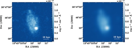
The uvw2 filter image of galaxy I.D. 23 (KUG 1343+270) shown before (left) and after (right). On the left is the galaxy at the original spatial sampling and resolution and on the right is the galaxy at the W3 sampling and resolution. While general morphology still resolvable at both resolutions, the level of detail is noticeably decreased.
4 KPC-SIZED STAR-FORMING REGIONS
4.1 Identification of star-forming regions
Molina et al. (2020b) detailed the method they used to define the kpc-sized star-forming regions in the galaxies that are the subject of our study. However, because our images are degraded to the WISE resolution, we redefined the regions at the new resolution. Following Molina et al. (2020b), we used dereddened, convolved, and reprojected H α surface brightness maps in conjunction with emission line diagnostic diagrams and H α equivalent widths to define the new resolved star-forming regions.
We adopted a minimum H α surface brightness, log[ΣH α/(erg s−1 kpc−2)] = 39, to locate areas dominated by light from H ii regions. This limit, recommended by Zhang et al. (2017), helps to identify pixels where H α emission is primarily due to recent star formation, as opposed to light from diffuse ionized gas (DIG). We also required that the H α equivalent width, EW(H α), be larger than 15 Å. EW(H α) is a mass-specific proxy for SFR, and is used here to mitigate the effect that diffuse galaxy light has on the identification of star-forming regions. These requirements mean that in all regions there should be a fairly high level of recent star formation.
We then followed the procedure of Molina et al. (2020b), which we summarize below, to delineate star-forming regions:
We identified local peaks in the surface brightness with log[ΣH α/(erg s−1 kpc−2)] ≥ 39.
We defined the largest isophote that corresponds to log[ΣH α/(erg s−1 kpc−2)] ≥ 39. If the contour has a diameter of less than 12 arcsec, which we set as the minimum allowed aperture size based on the resolution of the images, adopt a circular aperture 12 arcsec diameter.
We ensured that nebular emission line ratios from the region of interest fall outside of the AGN regions on each of the emission line diagnostic diagrams.
We repeated previous steps, shifting the contour levels in increments of 0.2 in log[ΣH α] and stopping at log[ΣH α/(erg s−1 kpc−2)] = 38, while ensuring that no region is identified more than once.
We calculated the diameter of the star-forming regions to ensure that they are still kpc sized.
To illustrate the results of this method, in Fig. 2, we show images of galaxy I.D. 13 (KUG 0757+468) in the four most relevant bands for our analysis. We outline the two identified star-forming regions in black. This figure includes an H α emission line flux map, the UVOT uvw2 and uvw1 images, and the WISE W3 image.
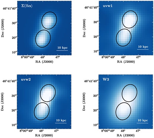
H α surface brightness map and uvw1, uvw2, and W3 images of galaxy I.D. 13 (KUG 0757+468). Each map or image has been convolved and reprojected to the W3 resolution. Outlined in black are the two identified star-forming regions in the galaxy.
Fig. 3 displays the location of all identified regions from all the galaxies on three emission line diagnostic diagrams (BPT), along with the extreme starburst lines and the composite line from Kewley et al. (2006) and Kauffmann et al. (2003) boundaries. While Molina et al. (2020b) find 56 star-forming regions across the 29 galaxies, at the lower resolution we are only able to identify 35 distinct star-forming regions. We list the locations of the 35 newly defined regions in Table 3, which also includes the corresponding regions identified by Molina et al. (2020b).
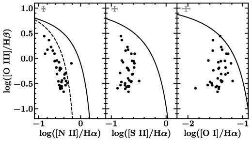
Emission line diagnostic diagrams for individual star-forming regions. The solid black line in each panel shows the extreme starburst limit from Kewley et al. (2006). The black dashed line represents the limit between the star-forming region and the composite object locus, from Kauffmann et al. (2003). Representative error bars can be found in the upper left corner of each plot. All star-forming regions, except for one, fall within the star-forming locus in each of the three diagrams.
Aperture definitions of the star-forming regions.
| Region | RA | Dec. | a | θ | Molina et al. (2020b) | |
|---|---|---|---|---|---|---|
| I.D. | (deg) | (deg) | (arcsec) | b/a | (deg) | region |
| (1) | (2) | (3) | (4) | (5) | (6) | (7) |
| 1.1 | 318.0262 | 11.3452 | 10.0 | 0.6 | 10 | 1.1, 1.2, 1.3 |
| 2.1 | 256.7246 | 32.1702 | 6.0 | 0.7 | 70 | 2.1 |
| 3.1 | 247.2359 | 39.6095 | 6.0 | 1.0 | – | 3.1 |
| 4.1 | 61.8478 | −6.6862 | 6.0 | 0.7 | 120 | 4.1 |
| 5.1 | 166.1879 | 45.1565 | 6.0 | 1.0 | – | 5.1 |
| 6.1 | 213.4954 | 43.8930 | 6.0 | 1.0 | – | 6.1 |
| 7.1 | 154.8364 | 46.5501 | 7.0 | 0.6 | 70 | 7.1, 7.2, 7.3 |
| 8.1 | 46.7492 | −0.8116 | 6.0 | 0.8 | 10 | 8.1 |
| 9.1 | 213.3655 | 43.9138 | 7.0 | 0.6 | 110 | 9.1, 9.2, 9.3 |
| 10.1 | 40.3040 | −0.8770 | 6.0 | 0.7 | 60 | 10.1, 10.2 |
| 11.1 | 225.1996 | 48.6075 | 6.0 | 1.0 | – | 11.1 |
| 12.1 | 115.2247 | 40.0697 | 6.0 | 0.8 | 170 | 12.1, 12.2, 12.3 |
| 13.1 | 120.1982 | 46.6922 | 6.0 | 0.8 | 160 | 13.1 |
| 13.2 | 120.1999 | 46.6888 | 6.0 | 0.8 | 160 | 13.3 |
| 14.1 | 220.1605 | 53.4781 | 6.0 | 1.0 | – | 14.1 |
| 15.1 | 44.1697 | −0.2460 | 6.5 | 0.8 | 140 | 15.1 |
| 16.1 | 118.1210 | 49.8397 | 6.0 | 1.0 | – | 16.1, 16.2 |
| 17.1 | 118.8558 | 48.4385 | 6.0 | 1.0 | – | 17.1 |
| 18.1 | 165.1179 | 44.2610 | 7.0 | 0.6 | 40 | 18.1 |
| 19.1 | 119.9948 | 31.8934 | 6.0 | 1.0 | – | 19.1 |
| 20.1 | 171.1020 | 23.6490 | 6.0 | 1.0 | – | 20.1 |
| 20.2 | 171.1057 | 23.6495 | 6.0 | 1.0 | – | 20.3 |
| 21.1 | 248.1097 | 39.5177 | 6.0 | 1.0 | – | 21.1 |
| 22.1 | 137.9836 | 27.8992 | 6.0 | 1.0 | – | 22.1 |
| 23.1 | 206.4690 | 26.7726 | 6.0 | 1.0 | – | 23.2, 23.4 |
| 23.2 | 206.4710 | 26.7770 | 6.0 | 1.0 | – | 23.1 |
| 24.1 | 178.3380 | 52.3455 | 6.0 | 1.0 | – | 24.1, 24.2 |
| 25.1 | 247.1632 | 40.1255 | 8.0 | 0.5 | 140 | 25.2, 25.3, 25.4 |
| 25.2 | 247.1626 | 40.1220 | 6.0 | 1.0 | – | 25.6 |
| 25.3 | 247.1675 | 40.1235 | 6.0 | 1.0 | – | 25.5 |
| 26.1 | 154.7685 | 46.4544 | 6.0 | 1.0 | – | 26.2, 26.3 |
| 26.2 | 154.7715 | 46.4515 | 10.0 | 0.4 | 90 | 26.1, 26.5 |
| 27.1 | 176.1242 | 55.5785 | 8.0 | 0.5 | 0 | 27.1 |
| 28.1 | 113.4005 | 45.9434 | 6.0 | 1.0 | – | 28.1 |
| 29.1 | 46.7171 | −0.8966 | 6.0 | 1.0 | – | 29.1 |
Notes. Column 1: The I.D. associated with each region. Column 2: Right ascension in degrees. Column 3: Declination in degrees. Column 4: Semimajor axis in arcseconds. Column 5: Ratio of semiminor axis to semimajor axis. Column 6: Angle of region with respect to vertical in degrees. Column 7: Molina et al. (2020b) region I.D.(s) that is/are included in region.
4.2 Properties of star-forming regions
We calculated the strength of the 4000 Å break, i.e. Dn(4000), for each region using maps in the SwiM VAC that were convolved and reprojected to the W3 band resolution (SwiM VAC; Molina et al. 2020a). Here, we used the relation Dn(4000) = fν,red/fν,blue, where fν,red and fν,blue refer to the average flux densities over the rest-frame wavelength ranges of 4000–4100 and 3850–3950 Å, respectively. Uncertainties on Dn(4000) were drawn from MaNGA uncertainty maps and include the systematic uncertainties described by Westfall et al. (2019). Molina et al. (2020b) caution against using the Battisti et al. (2016) attenuation law in regions with Dn(4000) > 1.3. In later analysis, we flagged regions with values greater than 1.3, and any composite regions that were made up of multiple regions previously identified by Molina et al. (2020b) where any of the initial regions had large Dn(4000) values. We checked our new Dn(4000) values against those found by Molina et al. (2020b) for their regions, and found that, within each galaxy, our values were comparable.
We also calculated the gas-phase metallicity for each region using the [N ii]/[O ii] ratio as described by Kewley & Dopita (2002). The [N ii]/[O ii] ratio is a useful metallicity diagnostic for regions with 12 + log(O/H) > 8.5, and has no dependence on ionization parameter (Kewley & Dopita 2002). It is also relatively insensitive to the presence of DIG (Zhang et al. 2017). We used emission line maps provided in the SwiM VAC that were convolved and reprojected to the WISE W3 resolution. Errors in the gas-phase metallicity were estimated from the spread of curves seen in fig. 3 of Kewley & Dopita (2002) to be ∼0.1, given that our minimum measured gas-phase metallicity was 8.59. The estimated error was dominated by this uncertainty, as uncertainties in the MaNGA maps and the systematic uncertainty in emission line flux as described by Belfiore et al. (2019) were both small in comparison.
Both the Dn(4000) and gas-phase metallicity measurements for individual regions are provided in Table 4.
Derived quantities for star-forming regions.
| Region | Galactocentric distance | Area | ||||
|---|---|---|---|---|---|---|
| I.D. | (kpc) | (kpc2) | IRX | β | 12 + log([O/H]) | Dn(4000) |
| (1) | (2) | (3) | (4) | (5) | (6) | (7) |
| 1.1 | 0.6 | 31.1 | 0.21 ± 0.3 | −1.26 ± 0.2 | 8.59 ± 0.1 | 1.31 ± 0.06 |
| 2.1 | 5.1 | 51.5 | 0.23 ± 0.3 | −1.09 ± 0.2 | 8.7 ± 0.1 | 1.23 ± 0.12 |
| 3.1 | 0.9 | 123.8 | 0.66 ± 0.3 | −1.13 ± 0.2 | 8.94 ± 0.1 | 1.27 ± 0.05 |
| 4.1 | 2.3 | 78.3 | 0.33 ± 0.3 | −1.29 ± 0.2 | 8.79 ± 0.1 | 1.3 ± 0.05 |
| 5.1 | 0.4 | 23.6 | 0.76 ± 0.3 | −0.9 ± 0.2 | 9.05 ± 0.1 | 1.55 ± 0.06 |
| 6.1 | 0.5 | 113.5 | 0.23 ± 0.3 | −1.15 ± 0.2 | 8.73 ± 0.1 | 1.33 ± 0.04 |
| 7.1 | 0.4 | 48.2 | 0.37 ± 0.3 | −1.43 ± 0.2 | 8.83 ± 0.1 | 1.32 ± 0.03 |
| 8.1 | 0.6 | 75.3 | 0.43 ± 0.3 | −1.07 ± 0.2 | 8.88 ± 0.1 | 1.28 ± 0.05 |
| 9.1 | 0.8 | 152.0 | 0.28 ± 0.3 | −1.37 ± 0.2 | 8.82 ± 0.1 | 1.26 ± 0.04 |
| 10.1 | 0.2 | 83.7 | 0.55 ± 0.3 | −1.03 ± 0.2 | 8.81 ± 0.1 | 1.26 ± 0.06 |
| 11.1 | 0.4 | 126.7 | 0.91 ± 0.3 | −0.7 ± 0.2 | 8.97 ± 0.1 | 1.4 ± 0.07 |
| 12.1 | 0.8 | 151.3 | 0.13 ± 0.3 | −1.43 ± 0.2 | 8.66 ± 0.1 | 1.13 ± 0.01 |
| 13.1 | 5.7 | 31.7 | 0.46 ± 0.3 | −1.26 ± 0.2 | 8.79 ± 0.1 | 1.21 ± 0.02 |
| 13.2 | 5.3 | 31.7 | 0.61 ± 0.3 | −1.29 ± 0.2 | 8.73 ± 0.1 | 1.23 ± 0.02 |
| 14.1 | 0.2 | 88.1 | 1.37 ± 0.3 | −0.48 ± 0.2 | 8.9 ± 0.1 | 1.46 ± 0.07 |
| 15.1 | 1.3 | 31.2 | 0.54 ± 0.3 | −1.3 ± 0.2 | 8.89 ± 0.1 | 1.22 ± 0.01 |
| 16.1 | 5.4 | 55.9 | 0.92 ± 0.3 | −0.97 ± 0.2 | 8.98 ± 0.1 | 1.47 ± 0.07 |
| 17.1 | 0.2 | 33.4 | 1.0 ± 0.3 | −1.03 ± 0.2 | 9.09 ± 0.1 | 1.46 ± 0.03 |
| 18.1 | 0.6 | 74.5 | 1.66 ± 0.3 | −0.96 ± 0.2 | 8.94 ± 0.1 | 1.45 ± 0.05 |
| 19.1 | 0.3 | 173.3 | 1.03 ± 0.3 | −0.67 ± 0.2 | 9.05 ± 0.1 | 1.28 ± 0.03 |
| 20.1 | 8.0 | 48.4 | 0.53 ± 0.3 | −1.42 ± 0.2 | 8.97 ± 0.1 | 1.33 ± 0.03 |
| 20.2 | 8.5 | 48.4 | 0.65 ± 0.3 | −1.14 ± 0.2 | 8.97 ± 0.1 | 1.33 ± 0.03 |
| 21.1 | 0.5 | 63.4 | 0.67 ± 0.3 | −1.25 ± 0.2 | 9.11 ± 0.1 | 1.59 ± 0.04 |
| 22.1 | 1.2 | 226.5 | 0.88 ± 0.3 | −0.68 ± 0.2 | 9.01 ± 0.1 | 1.3 ± 0.03 |
| 23.1 | 13.7 | 81.8 | 0.54 ± 0.3 | −1.37 ± 0.2 | 8.97 ± 0.1 | 1.26 ± 0.03 |
| 23.2 | 8.4 | 81.8 | 0.8 ± 0.3 | −1.16 ± 0.2 | 9.13 ± 0.1 | 1.41 ± 0.03 |
| 24.1 | 3.7 | 133.1 | 0.76 ± 0.3 | −0.79 ± 0.2 | 9.04 ± 0.1 | 1.27 ± 0.03 |
| 25.1 | 8.6 | 42.0 | 0.86 ± 0.3 | −1.36 ± 0.2 | 8.93 ± 0.1 | 1.31 ± 0.02 |
| 25.2 | 10.0 | 47.2 | 0.83 ± 0.3 | −1.33 ± 0.2 | 8.99 ± 0.1 | 1.3 ± 0.03 |
| 25.3 | 11.6 | 47.2 | 0.84 ± 0.3 | −1.33 ± 0.2 | 8.99 ± 0.1 | 1.31 ± 0.03 |
| 26.1a | 13.4 | 56.4 | – | – | 8.87 ± 0.1 | 1.2 ± 0.01 |
| 26.2a | 12.1 | 62.7 | – | – | 8.91 ± 0.1 | 1.24 ± 0.02 |
| 27.1 | 6.1 | 336.9 | 1.16 ± 0.3 | −0.22 ± 0.2 | 8.97 ± 0.1 | 1.72 ± 0.08 |
| 28.1 | 3.1 | 242.5 | 1.29 ± 0.3 | −0.84 ± 0.2 | 9.0 ± 0.1 | 1.27 ± 0.01 |
| 29.1 | 0.4 | 386.5 | 0.74 ± 0.3 | −1.38 ± 0.2 | 9.08 ± 0.1 | 1.4 ± 0.03 |
Notes. Column 1: Region I.D. Column 2: Distance of region from the nominal centre of the galaxy in kpc. Column 3: Area of the region in kpc2. Column 4: Calculated value of IRX. Column 5: Calculated value of β. Column 6: Gas-phase metallicity. We calculate this using the [N ii]/[O ii] ratio, as described by Kewley & Dopita (2002). Column 7: The systematic uncertainty in Dn(4000) as reported by Westfall et al. (2019) is included in the reported error.
aWe do not calculate values for galaxy 26 that rely on Swift/UVOT measurements due to the supernova light that contaminates the image.
4.3 The IRX–β relation
4.3.1 Calculation of β
We calculated β following the same procedure as Molina et al. (2020b). First, we simulated a 100 Myr continuous star formation continuum model using starburst99 (Leitherer et al. 1999), with an SFR of 1 M⊙ yr−1. The resulting SED was then redshifted to the frame of each galaxy and reddened to a range of E(B − V) values using the Battisti et al. (2016) attenuation law. We then measured β as a function of E(B − V) for the simulated SED using the 10 continuum windows defined by Calzetti et al. (1994).
We calculated the uvw2–uvw1 colour for each redshifted SED using the UVOT filter transmission curves. These curves, as well as an example redshifted and reddened SED, can be seen in fig. 1 of Molina et al. (2020b). Notably, the uvw2 and uvw1 transmission curves fit along either side of 2175 Å, allowing them to measure UV colour in a way that is not affected by the strength of the 2175 Å bump in the underlying attenuation curve. Finally, we measured the uvw2−uvw1 colour for each of our identified star-forming regions and inferred their β values by using the results of the simulations described above. These β values can be found in Table 4. We also converted our values of β to βGALEX, i.e. the values β would have had if they were measured via the FUV and NUV filters of GALEX (Martin et al. 2005) using the relationship defined by Molina et al. (2020b). See section 4.3 of Molina et al. (2020b) for further discussion of this conversion and its necessity. The error associated with this conversion represents the largest source of uncertainty in the calculation of β, and dominates the size of the error bars.
4.3.2 Calculation of IRX
The IRX is defined as the log of the ratio between the total IR luminosity and the FUV luminosity (Meurer et al. 1999). Here, we used the IR luminosity in the W3 band to determine the total IR luminosity, following the scaling relation defined by Cluver et al. (2017). This relationship connects the monochromatic luminosity at 12 µm to the total IR luminosity via log LTIR = 0.889log L12 µm + 2.21. Cluver et al. (2017) found that this relation predicts LTIR well in normal galaxies. This conversion represented the largest single source in error in the calculation of the IRX for each region, with an uncertainty of ∼0.2 dex. Additional uncertainties in flux measurements accounted for the additional ∼0.1 dex in the error calculation. To verify the applicability of the relation from Cluver et al. (2017), we measured flux values for each region in each of the WISE bands (W1, W2, W3, and W4). We then normalized these by the flux in the W3 band and plotted the resulting SED. As shown in Fig. 4, in both the plots of normalized flux density against frequency and νFν against frequency, emission at frequencies lower (and thus wavelengths longer) than the W3 band dominates. While the SED shape diverges primarily at higher frequencies, the bulk of the observed flux is emitted at lower frequencies, probed by W3 and W4. Thus, we concluded that the Cluver et al. (2017) relation is sufficient to estimate LTIR for our analysis.
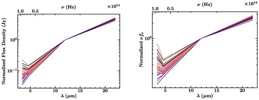
We plot flux values in the star-forming regions in each of the WISE bands. On the left is the normalized flux density plotted against the wavelength, and on the right is normalized νFν against wavelength. We normalize each value by the flux in the W3 band for each region. We do this to test the validity of using a relationship between L12 and LTIR for our regions. We see that, generally, the shapes are similar and appear to diverge mostly at short wavelength, but that most of the flux is in the portions of the SED at longer wavelength, where W3 and W4 are located.
We also calculated the FUV luminosity density at 1600 Å for each star-forming region. Since UVOT only has NUV filters, we translated the flux from the filter with the shortest wavelength, uvw2 (λcent = 1928 Å), to that at 1600 Å. To convert between the fluxes at 1928 and 1600 Å, we assumed that the two fluxes were related through F1600 = F1928(1600/1928)β, effectively assuming that the observed UV continuum follows a power law of the form F(λ) ∝ λβ in the wavelength range 1250 Å ≤ λ ≤ 2650 Å (Calzetti et al. 1994). We used the calculated β value for each region to scale our uvw2 flux measurements appropriately.
The calculated total IR luminosity and the luminosity density at 1600 Å were then used to find IRX values for each region following IRX ≡ log(LTIR/LFUV) (Meurer et al. 1999). IRX values for each region can be found in Table 4.
4.3.3 Fitting the IRX–β relation
We combined our measured values for IRX and β for each of the regions to examine the relationship between the two. We show the resulting IRX–β relation and its best fit in Fig. 5. The relation was fitted using non-linear least-squares regression to the functional form given by Meurer et al. (1999), allowing all three free parameters to be free to vary simultaneously. We obtained
where βreg is the NUV slope for that region (the free parameters are a = 1.51, b = 3.33, and c = 0.15).
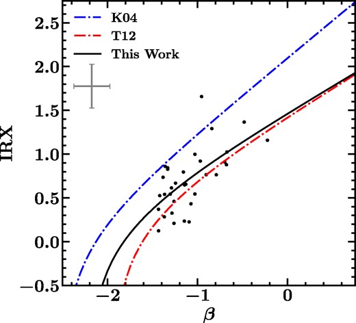
Star-forming regions in IRX–β space compared to relationships for starburst galaxies (blue dot-dashed line; Kong et al. 2004) and local galaxies (red dot–dashed line; Takeuchi et al. 2012). Additionally, we plot our best-fitting relationship given in equation (2) (solid black line). Representative error bars can be found in the upper left corner. We find that our star-forming regions follow a relationship similar to that followed by the local galaxies sampled by Takeuchi et al. (2012).
Fig. 5 also shows other IRX–β relationships for local and starburst galaxies (Kong et al. 2004; Takeuchi et al. 2012). We note that our best-fitting relationship is similar to the one determined by Takeuchi et al. (2012) for the integrated light from local galaxies. Our points have a large scatter about the best-fitting relation, but seem to follow expected relationships for integrated galaxy light. The scatter of the star-forming regions about the relationship, however, is greater than can be attributed to the size of the error bars alone. The scatter is similar to that shown in other studies of this kind, both on galactic (e.g. Kong et al. 2004; Takeuchi et al. 2012; Nagaraj et al. 2021) and sub-galactic scales (e.g. Boquien et al. 2012).
In Fig. 6, we compare the IRX–β relationship for the integrated light of our sample of galaxies to that for the individual star-forming regions. We fitted the integrated galaxy light data following the same procedure as for the individual regions to obtain a relationship of the same functional form as equation (2), but for the NUV slope for integrated galaxy light, namely
(the free parameters are a = 1.473, b = 2.889, and c = 0.507).
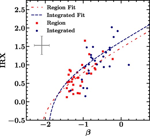
The IRX–β relation for star-forming regions (red squares and dot–dashed line) and for integrated galaxy light (blue circles and dashed line). Best fits found through non-linear least-squares regression are noticeably similar for both the individual regions (see equation 2) and integrated galaxy light (see equation 3). The representative error bar for each set of points is plotted in the upper left, and is the same for both integrated galaxy light and light from individual regions. This is because the dominant source of error in the IRX arises from the conversion between W3 luminosity and LTIR and the dominant source of error in β arises from conversion to βGALEX. These sources of error are present and dominant in the measurements for the galaxies as a whole and the individual regions. We find that star-forming regions and integrated galaxy light from their hosts tend to follow very similar IRX–β relations.
We find that individual regions and integrated galaxy light seem to follow very similar IRX–β relations. This effect may be a result of the size of our regions – due to the resolution of the WISE W3 band, our minimum aperture size is fairly large and our regions can encompass significant portions of their host galaxies.
4.3.4 Effect of S/N on β and IRX
All observed galaxies had a minimum S/N of 15 in the integrated galaxy light for both Swift/UVOT filters used, and similarly a minimum S/N of 10 in the WISE W3 band. If we were to apply a more stringent cut on the S/N of the galaxies, neither the level of scatter seen in IRX and β nor the overall best-fitting relation would change significantly. This means that the scatter we see is not a result of our choice in S/N but is likely intrinsic. When we investigate the effect of stricter S/N requirements on other properties of the regions, we tend to find a marginally higher average SFR, although the average gas-phase metallicity of the regions does not change. Hence, we conclude that imposing more stringent S/N cuts does not change our conclusions.
5 DEPENDENCE OF THE IRX–β RELATION ON PHYSICAL PARAMETERS
We investigated the relationship between IRX and β for our star-forming regions by comparing the results with a number of other properties, including galaxy inclination, measured by taking the ratio of the observed minor and major axes, the galactocentric radius, area, SFR, age, as measured by Dn(4000), and gas-phase metallicity of each region. We show colour-coded plots to illustrate the effect of each of these properties in Fig. 7.
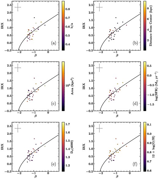
IRX–β points coloured by a number of observable parameters. We check correlations between (a) inclination, measured by b/a, (b) galactocentric distance in kpc, (c) area of the region in kpc2, (d) the SFR, (e) the average stellar age of the region, measured by Dn(4000), and (f) the gas-phase metallicity of the region. The characteristic error bars for the regions are shown in the upper left corner. We find that the most convincing correlations exist between IRX–β and Dn(4000) and IRX–β and gas-phase metallicity.
We investigated the effect of inclination on the IRX–β relationship in Fig. 7(a). We found that while there is no overall relationship between the inclination of the galaxy and the IRX–β relationship, inclination may explain the location of region 18.1. This region has the largest IRX value of our sample, and lies furthest from the locus of points in both Figs 5 and 7(a). Its host galaxy is also the most inclined of our sample, with b/a = 0.33. Salim & Boquien (2019) note that galaxies with b/a values less than 0.3 tend to fall significantly above the IRX–β relation and exhibit more scatter than galaxies that are face-on. While this region has a value slightly above the threshold listed by Salim & Boquien (2019), it is sufficiently close to that limit to explain the increased scatter from the best-fitting relation. Aside from this object, however, a Spearman rank order test showed no evidence for a correlation of IRX or β with inclination, with p-values, which represent the probability that the observed correlation is due to chance, of 0.79 and 0.97, respectively. We also note that our sample seems to be biased towards galaxies that are face-on. Further analysis on a more balanced sample of inclinations would be needed to confirm this lack of relation.
Because dust attenuation is known to decrease with increasing galactocentric radius, we explored the effect of position within a galaxy on a star-forming region’s location in the IRX–β diagram, and show the results in Fig. 7(b). IRX and galactocentric distance have a Spearman rank order test p-value of 0.82, meaning that there is no statistically significant correlation between the two. We find that β and galactocentric distance have a Spearman correlation coefficient of −0.32 and a p-value of 0.07, which is nearly, but not quite 2σ significance. This potential negative correlation implies that as galactocentric distance increases, β becomes more negative.
Given the lower resolution of our final images, some newly defined regions are no longer kpc sized, but are rather of the order of 10 kpc across. We therefore plotted the relationship between the size of a region and its IRX and β values to see what effect, if any, the larger apertures have on the measured properties. The results are shown in Fig. 7(c). When we performed statistical analysis, we found that there is no convincing trend between the area of a region and its value of IRX or β. The associated p-values from the Spearman rank order test were 0.28 and 0.59, respectively.
The effect of aperture size on the relation can also be explored by comparing the IRX–β relation found for individual star-forming regions with the relation found for integrated galaxy light. We compared these relations in Fig. 6. We see in that figure that IRX–β measurements for integrated galaxy light follow a very similar relationship to the light from individual star-forming regions. We also see that integrated galaxy light tends to have both more positive β values and higher IRX. The median values of IRX and β for the integrated galaxy light are 1.05 and −0.74, respectively, whereas those values for the regions are 0.59 and −1.29. This represents a statistically significant difference between the values measured for individual regions and those measured for the galaxy as a whole. This finding is reasonable given that older stellar populations, increased dust content, or a combination thereof could create redder IRX and β measurements in the integrated galaxy light.
We calculated the SFR of each region, and plotted it with IRX and β to see whether a convincing relationship existed between SFR and IRX–β in Fig. 7(d). The SFR was measured using the relationship for dereddened H α luminosity as described by Kennicutt & Evans (2012). We do not find statistically significant relationships between SFR and IRX or β. The p-values measured for these potential correlations are 0.20 and 0.85, respectively.
The amplitude of the 4000 Å break can be used as a proxy for stellar age (Balogh et al. 1999). Generally as light from older stars becomes more prominent, implying an increased average stellar age, Dn(4000) also increases. We colour the points in our IRX–β diagram according to their calculated Dn(4000) values in Fig. 7(e). When we calculate correlation coefficients for IRX and Dn(4000), and β and Dn(4000), we find that IRX and Dn(4000) have a moderate positive correlation, with a Spearman correlation coefficient of 0.54, and a p-value of 0.001. We also find a slightly weaker positive correlation between Dn(4000) and β. These two variables have a Spearman correlation coefficient of 0.35 and a p-value of 0.04. This means that IRX and Dn(4000) are statistically correlated at the 99.9 per cent confidence level, and β and Dn(4000) are correlated at the 96 per cent confidence level. We show the relationship between Dn(4000) and β and Dn(4000) and IRX in Fig. 8. We also investigate the relationship between IRX–β and another stellar age indicator, the HδA Lick index (Worthey & Ottaviani 1997). We use convolved and reprojected SwiM VAC flux and continuum maps to calculate this index for each of our regions, following the equation defined in section 5.4 of Molina et al. (2020a). Similarly to Dn(4000), we find a strong correlation between IRX and that index, showing that older stellar populations have higher values of IRX.
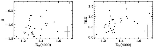
We show the relationships between Dn(4000) and β (left) and Dn(4000) and IRX (right). The average uncertainties in each figure are represented by the error bars in the upper left of each plot. We note a fairly strong correlation between IRX and Dn(4000), with a Spearman correlation coefficient of 0.54 and a p-value of 0.001, and a weaker correlation between β and Dn(4000) with a Spearman correlation coefficient of 0.35 and a p-value of 0.04.
The positive correlations between the 4000 Å break and both IRX and β imply that older stellar populations tend to look redder in the IRX–β space, and also might follow steeper attenuation curves. This is reasonable given that in regions with older average stellar populations, light from evolved stars becomes more prominent relative to the emission at 1600 Å, which tends to probe younger stellar populations. This is also consistent with the general result from Molina et al. (2020b), who found that older regions tended to lie above the expected β–|$\tau ^{l}_\mathrm{ B}$| relationship.
We further investigated the difference between regions with Dn(4000) > 1.3 and those with values <1.3, as Molina et al. (2020b) found that those regions behave differently in |$\tau ^l_\mathrm{ B}$|–β space. In the IRX–β relation, we do not find a significant difference in behaviour between these two populations. Median β values for the two populations are essentially the same and median IRX values for the two populations are separated by 0.15, where the group with Dn(4000) > 1.3 has a higher IRX value. This difference, however, is smaller than the size of the individual error bar.
Finally, we explored the effect of gas-phase metallicity on the IRX–β relationship. We calculated gas-phase metallicity using the [N ii]/[O ii] relationship defined by Kewley & Dopita (2002), and corrected for internal reddening using the Balmer decrement. The plot of metallicity as a function of IRX–β is shown in Fig. 7(f). We found that while β and metallicity do not have a statistically significant relationship, and have a p-value for correlation of 0.08, IRX and metallicity are strongly positively correlated, with a Spearman correlation coefficient of 0.67 and a p-value of 2.07 × 10⁻⁵. These two relationships are plotted in Fig. 9.
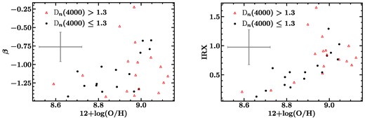
We show the relationships between metallicity and β (left) and metallicity and IRX (right), split by stellar age. Regions with Dn(4000) > 1.3 are shown as red triangles and regions with Dn(4000) ≤ 1.3 are shown as black circles. The systematic uncertainties in each figure are represented by the error bars in the upper left of each plot. When all regions are included, we do not find a statistically significant correlation between metallicity and β, but do find a strong positive correlation between metallicity and IRX. When old regions, with Dn(4000) > 1.3, are excluded, the scatter in both plots is noticeably smaller. We also recover strong positive correlations between IRX and metallicity and β and metallicity when the older populations are excluded.
We also investigated the potential influence of aging stellar populations on our observed correlation between IRX and metallicity. To disentangle this effect, we separate the regions into those with Dn(4000) ≤ 1.3 and Dn(4000) > 1.3 as before, and measure correlations between the populations and IRX, β, and metallicity. When older stellar populations, those with Dn(4000) > 1.3, are excluded, we find that the strength of the positive IRX–metallicity correlation is increased, with a Spearman correlation coefficient of 0.82 and a p-value of 9.84 × 10⁻⁵. Notably, we also recover a statistically significant, strong positive correlation between β and metallicity, with a Spearman correlation coefficient of 0.55 and a p-value of 0.028. We show this effect in Fig. 9, where older populations are shown as red triangles and younger populations are shown as black circles. The scatter in the correlations between IRX and metallicity and β and metallicity is noticeably smaller when older populations are excluded.
The correlation between metallicity and the IRX strongly implies that the shape of the attenuation law for a region is influenced by the metallicity of that region. This result is consistent with the correlation between metallicity and IRX found by Shivaei et al. (2020) in their sample of z ∼ 2–2.5 galaxies, as well as the result found by Boquien et al. (2009) for sub-kpc-sized star-forming regions within eight star-forming galaxies. The metallicity dependence thus appears to exist independent of aperture size. This result implies that the attenuation curve is steeper for galaxies with higher metallicities, whereas lower metallicity regions have greyer attenuation curves. Physically, this suggests that galaxies with lower metallicity have different dust grain compositions and thus attenuation curves than those with higher metallicity.
6 DISCUSSION AND CONCLUSIONS
We examined the IRX–β relation using a sample of previously identified star-forming regions in 29 galaxies with both MaNGA and Swift/UVOT observations (Molina et al. 2020b). The sample is a subset of a larger catalogue that was created to investigate the quenching of star formation in nearby galaxies (Molina et al. 2020a). By supplementing the MaNGA and Swift/UVOT data with WISE W3 measurements, we were able to compare the IRX with the UV spectral slope for both the entire galaxies and kpc-sized star-forming regions within the galaxies.
Integrated galaxy light follows the same IRX–β relationship as the light from resolved star-forming regions, although the integrated light has both higher values of IRX and more positive values of β. As a result, the curves that describe the IRX–β relationship for the individual regions and the integrated galaxy light are very similar. This similarity may be taken to suggest that the IRX–β relation that we observe in integrated galaxy light is driven by the contributions from star-forming regions to that light. Such a conclusion, however, is complicated by the relatively large minimum aperture size of our regions. The relationship we observe may be ultimately connected to the size of the apertures for a variety of reasons. The observed shift along the IRX–β relation between the regions and the integrated light may also be caused by a combination of effects, such as aging stellar populations in the galaxy outside of the regions and increased dust content within the regions. In addition, previous studies have found significant variations in attenuation curves at different radii within galaxies (e.g. Li et al. 2020). Our observed trend may be caused by some combination of changing attenuation and optical depths that, when seen together, mimics one attenuation curve. The large size of our star-forming regions might average over those radial effects, creating the impression that total galactic attenuation is driven by star-forming regions. This means that, in normal star-forming galaxies, kpc-scale star-forming regions are large enough to average sub-galactic processes into galactic-wide effects.
A number of properties, such as gas-phase metallicity (e.g. Boquien et al. 2009; Shivaei et al. 2020), stellar population age (e.g. Kong et al. 2004; Cortese et al. 2008), variations in star formation history (e.g. Kong et al. 2004; Narayanan et al. 2018), or variations in the underlying attenuation curve (e.g. Narayanan et al. 2018; Salim & Boquien 2019), have been invoked to explain the scatter in the IRX–β relationship. While we have a relatively small sample of 29 galaxies and 35 star-forming regions, we explore potential relationships between the IRX–β relation and a number of parameters. We find that the distance of the regions from the centre of their host galaxies, the area of the region, and the inclination of the galaxy have little effect on where points fall in IRX–β space, although we do note that the region with the largest IRX value has the smallest b/a value. Salim & Boquien (2019) note that edge-on galaxies tend to have higher IRX values and exhibit more scatter in the relationship than their face-on counterparts. We attribute the placement of the aforementioned galaxy to this effect. We also note that our sample is largely made up of face-on galaxies. This selection bias might also play a role in the lack of relationship between IRX–β and b/a that we see here.
We find no statistically significant relationship between SFR and β or IRX. Conversely, there is a moderate correlation between the value of Dn(4000) and the IRX, where higher values of Dn(4000) and thus older stellar populations appear to have higher IRX values. We also find a weaker, but still significant, correlation between β and Dn(4000). In contrast, we do not find any significant difference in the IRX–β relationship between populations of regions with values of Dn(4000) greater or less than 1.3, unlike the trend found by Molina et al. (2020b). We do, however, see a difference in the behaviour of these two populations in the IRX–metallicity and β–metallicity spaces.
Of the parameters we considered, we see the strongest correlation between IRX and the gas-phase metallicity, 12 + log(O/H). This is a strong positive correlation, where higher values of IRX correlate with higher metallicities. When regions with high values of Dn(4000) are excluded and only regions with younger average ages are considered, the correlation between IRX and metallicity becomes stronger, and a statistically significant relationship between β and metallicity is recovered. This result is consistent with previous work both in sub-kpc-sized star-forming regions and in samples of z ∼ 2–2.5 galaxies. Therefore, regardless of the aperture used, metal-rich regions will have steeper attenuation curves, whereas lower metallicity regions have greyer (i.e. flatter) attenuation curves. Observationally, this means that galaxies with higher metallicities should look redder than their lower metallicity counterparts.
Finally, we found that the scatter in IRX–β does not decrease with more stringent requirements in S/N. When viewed in conjunction with the lack of correlation between IRX–β and most of the physical parameters we investigate, we conclude that the scatter in IRX–β at kpc scales may be driven by intrinsic physical differences between different regions. These differences could largely be related to the gas-phase metallicity and the average stellar age of the regions, although the galactocentric radius may also contribute.
While our results are intriguing, they are somewhat limited due to our relatively small sample size. In a forthcoming paper, the second data release of the SwiM VAC (Molina et al. 2023) will expand the number of galaxies with both Swift/UVOT and MaNGA data from 150 to 559. This expanded sample will provide a significant increase in the number of star-forming galaxies available, and can be used to verify the trends noted here.
ACKNOWLEDGEMENTS
We thank the referee, Tsutomu T. Takeuchi, for his thorough reading of the manuscript and helpful comments.
This work was supported by the NASA Astrophysics Data Analysis Program (ADAP) through grant 80NSSC20K0436.
This work was supported by funding from Ford Foundation Postdoctoral Fellowship, administered by the National Academies of Sciences, Engineering, and Medicine, awarded to MM in 2021–2022. The work of MM was supported in part through a fellowship sponsored by the Willard L. Eccles Foundation.
RY acknowledges support by the Hong Kong Global STEM Scholar scheme, by the Hong Kong Jockey Club Charities Trust through the JC STEM Lab of Astronomical Instrumentation, and a grant from the Research Grants Council of the Hong Kong Special Administrative Region, China (Project No.: CUHK 14302522).
MB gratefully acknowledges support by the ANID BASAL project FB210003 and from the FONDECYT regular grant 1211000.
The Institute for Gravitation and the Cosmos is supported by the Eberly College of Science and the Office of the Senior Vice President for Research at the Pennsylvania State University.
Funding for the SDSS-IV has been provided by the Alfred P. Sloan Foundation, the U.S. Department of Energy Office of Science, and the Participating Institutions.
SDSS-IV acknowledges support and resources from the Center for High Performance Computing at the University of Utah. The SDSS-IV website is www.sdss4.org.
SDSS-IV is managed by the Astrophysical Research Consortium for the Participating Institutions of the SDSS Collaboration including the Brazilian Participation Group, the Carnegie Institution for Science, Carnegie Mellon University, Harvard–Smithsonian Center for Astrophysics, the Chilean Participation Group, the French Participation Group, Instituto de Astrofísica de Canarias, the Johns Hopkins University, Kavli Institute for the Physics and Mathematics of the Universe (IPMU)/University of Tokyo, the Korean Participation Group, Lawrence Berkeley National Laboratory, Leibniz Institut für Astrophysik Potsdam (AIP), Max-Planck-Institut für Astronomie (MPIA, Heidelberg), Max-Planck-Institut für Astrophysik (MPA, Garching), Max-Planck-Institut für Extraterrestrische Physik (MPE), National Astronomical Observatories of China, New Mexico State University, New York University, University of Notre Dame, Observatário Nacional/MCTI, the Ohio State University, Pennsylvania State University, Shanghai Astronomical Observatory, United Kingdom Participation Group, Universidad Nacional Autónoma de México, University of Arizona, University of Colorado Boulder, University of Oxford, University of Portsmouth, University of Utah, University of Virginia, University of Washington, University of Wisconsin, Vanderbilt University, and Yale University.
This research has made use of the NASA/IPAC Infrared Science Archive, which is funded by the NASA and operated by the California Institute of Technology.
DATA AVAILABILITY
The SwiM VAC is publicly available at the following link: https://www.sdss4.org/dr17/data_access/value-added-catalogs/?vac_id=swift-manga-value-added-catalog
WISE observations of the galaxies mentioned here can be publicly accessed through the NASA/Infrared Processing and Analysis Center (IPAC) Infrared Science Archive at the following link: https://irsa.ipac.caltech.edu/frontpage/
