


ABSTRACT
The local galaxy peculiar velocity field can be reconstructed from the surrounding distribution of large-scale structure and plays an important role in calibrating cosmic growth and expansion measurements. In this paper, we investigate the effect of the stochasticity of these velocity reconstructions on the statistical and systematic errors in cosmological inferences. By introducing a simple statistical model between the measured and theoretical velocities, whose terms we calibrate from linear theory, we derive the bias in the model velocity. We then use lognormal realizations to explore the potential impact of this bias when using a cosmic flow model to measure the growth rate of structure, and to sharpen expansion rate measurements from host galaxies for gravitational wave standard sirens with electromagnetic counterparts. Although our illustrative study does not contain fully realistic observational effects, we demonstrate that in some scenarios these corrections are significant and result in a measurable improvement in determinations of the Hubble constant compared to standard forecasts.
1 INTRODUCTION
The peculiar velocity field is an important ingredient in modern cosmological observations of the growth and expansion of the Universe, encoding information about gravitational physics, and adding noise to the smooth Hubble flow. In both cases, reconstructions of the peculiar velocity field based on the observed large-scale structure play an important role, and therefore errors in these reconstructions can introduce both statistical and systematic errors to cosmological inferences. In this paper, we will consider a new general model for these error distributions, and present a first analysis of its impact on associated growth and expansion measurements.
Accurately measuring the redshift of the associated host galaxy of a distance indicator is a problem that all approaches to local measurements of the Hubble constant H0 face, and is an unavoidable source of error (Davis et al. 2019; Pesce et al. 2020). The cosmological redshift of a galaxy will be distorted by its peculiar velocity and in the local Universe, where galaxy peculiar velocities are not negligible compared to the recession velocity due to the expansion of the Universe, is an important source of uncertainty in measurements of H0. Recent work by Carr et al. (2022) and Peterson et al. (2022) has explored how improving redshift measurements, and more comprehensive modelling of the peculiar velocity component of redshift, can impact Type Ia supernova cosmology using Pantheon+ light curves (Scolnic et al. 2022).
The local peculiar velocity field is typically modelled from galaxy redshift survey data in order to predict the galaxy peculiar velocity (Dekel, Bertschinger & Faber 1990; Willick et al. 1997; Zaroubi, Hoffman & Dekel 1999; Lavaux 2016), which is then subtracted from the measured host redshift to theoretically ‘correct’ it and thus recover the actual cosmological redshift of the source (Willick & Batra 2001; Boruah, Hudson & Lavaux 2021). Comparisons between the measured velocity field – estimated from observations of the peculiar velocities of local galaxies – and the predicted velocity and density fields – inferred from galaxy redshift surveys – also allow us to constrain the cosmological matter density parameter Ωm and subsequently the growth rate of structure f (Strauss & Willick 1995; Pike & Hudson 2005; Carrick et al. 2015; Said et al. 2020; Lilow & Nusser 2021; Courtois et al. 2023). Given the importance of the modelled peculiar velocity in determinations of H0 and f, we must also be conscious of any systematic or statistical error inherent to the creation of the model velocity field and how these errors may be propagated into cosmological measurements. Hollinger & Hudson (2021) investigate several facets of this approach, including choice of smoothing length and density tracer as well as the effects of noise. Close consideration of the linear theory commonly used to create the model velocity field from the galaxy density field reveals that the recovered local velocity field is a biased reconstruction of the measured velocity field. By accounting for this bias, we can produce a model velocity field that matches observations, propagate this corrected model into our determinations of H0, and quantify the effect this improvement has on measurement accuracy.
The current expansion rate of the Universe, parameterized by H0, dictates key features of our Universe such as its size and age and is degenerate with parameters such as the dark energy equation of state, making H0 itself a uniquely interesting cosmological parameter. There are two major approaches used to measure H0, largely distinguished by the epoch of the Universe at which the measurement is made. Early-time measurements of H0 are made by jointly fitting a set of cosmological parameters to large-scale features such as the cosmic microwave background (CMB; Planck Collaboration VI 2020) and baryon acoustic oscillations (BAOs; Alam et al. 2021). Late-time measurements of H0 are reliant on distance indicators such as Type Ia supernovae (which act as standard candles) and a set of distance calibrations (i.e. parallax and Cepheid variables) that come together to form the local distance ladder. Other late-time measurements rely instead on the tip of the red giant branch (TRGB) as an important component of the distance ladder (Freedman et al. 2019).
Early-time predictions favour a smaller value of H0, the most notable being the 2018 results of CMB experiment Planck that find |$H_0 = 67.27\, \pm \, 0.60$| km s−1 Mpc−1 (Planck Collaboration VI 2020). Late-time predictions, however, favour larger values. One such recent measurement from the SH0ES team made with Hubble Space Telescope observations yields |$H_0 = 73.04\, \pm \, 1.04$| km s−1 Mpc−1 (Riess et al. 2022). A separate late-time measurement using the TRGB distance ladder finds H0 = 69.8 ± 0.6 (stat) ± 1.6 (sys) km s−1 Mpc−1 (Freedman 2021), a result within 2σ of SH0ES Cepheid calibrations and not statistically significant from CMB-inferred predictions. The discrepancy between measurements made at early and late times has led to introspection, and both approaches have been thoroughly probed for sources of systematic error, such as refining calibrations to the Cepheid distance ladder (Pietrzyński et al. 2019; Reid, Pesce & Riess 2019; Riess et al. 2019) and the TRGB distance ladder (Anand et al. 2022; Anderson, Koblischke & Eyer 2023; Hoyt 2023), as well as modifications to physics at both early times (Poulin et al. 2019; Kreisch, Cyr-Racine & Doré 2020; Jedamzik, Pogosian & Zhao 2021; Lin, Chen & Mack 2021) and late times (Zhao et al. 2017; Benevento, Hu & Raveri 2020) – with no explanation fully resolving the disparity between the two approaches. We are left with a disagreement of the order of 4–6σ, depending on the data considered, that cannot be immediately explained away by systematic effects, termed the ‘Hubble tension’ (see Di Valentino et al. 2021, and references therein).
Another alternative late-time approach to measuring H0 is through the use of gravitational waves (GWs) as standard sirens (Schutz 1986). The distance to the source can be determined directly from the gravitational waveform, and the redshift may be measured from accompanying electromagnetic data. This method produces complementary results to those obtained using standard candles while not being dependent on the local distance ladder, and thus independent of any systematic errors inherent to standard candle measurements. Only one such event, GW170817, has had an electromagnetic counterpart detected with high confidence, and this was used by Abbott et al. (2017) to obtain the measurement |$H_0 = 70.0^{+12.0}_{-8.0}$| km s−1 Mpc−1. It was then shown by Howlett & Davis (2020) that the choice of peculiar velocity for the host galaxy can significantly influence the resulting value of H0, and combining a Bayesian model averaging analysis with constraints on the viewing angle obtained from radio data find that |$H_0 = 64.8^{+7.3}_{-7.2}$| km s−1 Mpc−1. An analysis undertaken by Mukherjee et al. (2021b) applied statistical reconstruction techniques to obtain a peculiar velocity correction for the host galaxy of GW170817, and in combination with the same radio data find |$H_0 = 68.3^{+4.6}_{-4.5}$| km s−1 Mpc−1. Not only can the method used to account for the peculiar motion of galaxies influence the recovered value of H0, especially when trying to obtain a result from a single source at low redshift, but it can also significantly impact the uncertainty in the estimate.
In Section 2, we introduce our new statistical model for the errors resulting from a linear-theory reconstruction of the velocity field. In Section 3, we explore the effect of these errors on determinations of the growth rate of structure based on this reconstructed velocity field, and in Section 4 we discuss how the velocity field reconstruction affects determinations of H0, using a simulated sample of GW events with electromagnetic counterparts as distance indicators. We compare these simulated results to the expected error from analytical forecasts in Section 5. Finally, we summarize our results and discuss future applications of this work in Section 6.
2 A MODEL FOR THE ERRORS IN VELOCITY RECONSTRUCTION
Velocity reconstruction is the process of inferring the peculiar velocity field across a cosmic volume from the estimated density field within that volume, typically mapped by galaxy positions. In linear perturbation theory, neglecting redshift-space distortions, the i = (x, y, z) components of the peculiar velocity field |$v_i({\boldsymbol{ x}})$| are related to the matter overdensity field |$\delta _\mathrm{ m}({\boldsymbol{x}})$| via complex Fourier amplitudes:
in terms of the cosmic scale factor a, Hubble parameter H, and growth rate f, where ki are the components of wavevector |${\boldsymbol{ k}}$|. An example derivation of equation (1) can be found in appendix C of Adams & Blake (2017). The overdensity field is typically constructed by gridding a density-field tracer and smoothing the resulting distribution to reduce noise. If the tracer has a linear bias factor b, then the growth rate in equation (1) can be replaced by β = f/b. The accuracy of a linear-theory reconstruction model has been thoroughly investigated by many authors during the past two decades (e.g. Zaroubi et al. 1999; Berlind, Narayanan & Weinberg 2001; Okumura et al. 2014; Lavaux 2016; Hollinger & Hudson 2021). We note that in this study we will neglect the effect of redshift-space distortions, which shift the observed positions of galaxies as a function of the growth rate.
In Fig. 1, we show the result of applying equation (1) to reconstruct the model velocity field of a |$1 \, \mathrm{ h}^{-3}$| Gpc3 box of dark matter particles (b = 1) in today’s Universe (snapshot with redshift z = 0) created as part of the Gigaparsec WiggleZ N-body simulations (Poole et al. 2015), comparing the inferred velocity at each position with the underlying peculiar velocities of each particle in the simulation. This simulation is chosen as an illustrative example, since we seek to describe generic trends. In each case, we display the radial velocities of the particles relative to an observer. For the purposes of this test, we reconstructed the density field using 105 dark matter particles (where this number is chosen to create a non-negligible Poisson noise that we wish to model below) and sampled the velocity at the positions of 104 different particles. After binning the particles on a grid with dimension 1283, we applied a Gaussian smoothing to the density field with r.m.s. |$\lambda = 10 \, \mathrm{ h}^{-1}$| Mpc as our fiducial choice, where we also compare results assuming λ = 5 and |$20 \, \mathrm{ h}^{-1}$| Mpc. After applying equation (1), we imposed the appropriate complex conjugate properties on the velocity field. The result of the reconstruction is the characteristic distribution of Fig. 1, where the scatter is driven by breakdown of equation (1) (i.e. non-linear velocities) and Poisson noise in the density field.
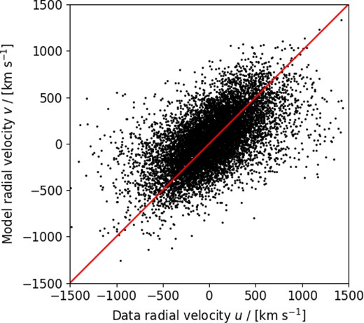
A comparison of the radial velocities u of 104 dark matter particles within a |$1 \, \mathrm{ h}^{-3}$| Gpc3 simulation box, and the model values v at these positions applying linear-theory reconstruction to the density field in the box. The diagonal solid line indicates v = u, about which the values show a significant scatter.
In this study, we introduce a phenomenological statistical model to characterize the inaccuracies in the reconstructed velocity field. We show that the coefficients of this model may be related to relevant physical effects and used to correct biases in the reconstructed velocity field, as a useful alternative to full non-linear modelling. Fig. 1 motivates a 2D elliptical Gaussian statistical model for the reconstructed model velocity component v and the measured velocity component u, where the joint probability can be expressed as:
in terms of the variance of v, |$\sigma _v^2 = \langle v^2 \rangle$|, the variance of u, |$\sigma _u^2 = \langle u^2 \rangle$|, and the cross-correlation coefficient |$r = \sigma _{uv}^2/(\sigma _u \, \sigma _v)$|, where |$\sigma _{uv}^2 = \langle u \, v \rangle$|. We assume that the variables have zero mean by isotropy, 〈u〉 = 〈v〉 = 0. The statistical relation between the model velocity v and measured velocity u is hence characterized by the values of σu, σv, and r at every point. An immediate deduction from equation (2) is that, for a point with model velocity v, the mean measured velocity |$\overline{u} \ne {v}$|. In fact:
which can be considered as an unbiased model prediction at each point. Fig. 2 verifies the prediction of equation (3) by averaging the measured velocity of the 104 particles displayed in Fig. 1 in bins of the model velocity v. The errors in each bin are calculated as errors in the mean, |$\sigma /\sqrt{N}$|, where N is the number of particles in the bin and σ is the standard deviation of the velocity differences. We see that |$\overline{u} \ne {v}$|, and is well modelled by equation (3), where the coefficients σu, σv, and r are calculated as described below.
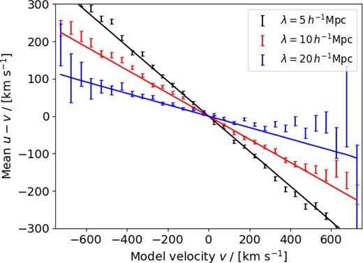
The mean difference between the radial velocity component of particles measured in the simulation and their value predicted by linear-theory reconstruction, binned as a function of model velocity. Results are shown for three different smoothing scales |$\lambda = (5, 10, 20) \, \mathrm{ h}^{-1}$| Mpc.
The errors in each bin are calculated as errors in the mean, and the solid line is the prediction of equation (3).
Linear theory gives us analytical expressions for the parameters of the model σu, σv, and σuv:
where V is the box volume, |$P({\boldsymbol{ k}})$| is the model matter power spectrum at wavenumber |${\boldsymbol{ k}}$|, |$D({\boldsymbol{ k}}) = \mathrm{ e}^{-k^2 \lambda ^2/2}$| is the Fourier transform of the damping kernel used to smooth the density field before applying the linear-theory velocity reconstruction, and n is the particle number density. Equation (4), the variance of the underlying field, is the standard expression for the velocity dispersion resulting from a given density power spectrum (Gorski 1988). Equation (5), the variance of the model velocity field, includes the additional effects of the shot-noise contribution to the power (1/n) and the damping of power resulting from the smoothing (|$D^2({\boldsymbol{ k}})$|). Equation (6), the cross-correlation between the two, includes just one power of the damping.
We evaluate equations (4)–(6) as a sum over a grid of Fourier modes, not as an integral over |${\boldsymbol{ k}}$|-space (|$\int \frac{\mathrm{ d}^3{\boldsymbol{ k}}}{(2\pi)^3} \rightarrow \frac{1}{V} \sum _{{\boldsymbol{ k}}}$|) because the inverse powers of k imply that the expressions are dominated by a small number of low-|${\boldsymbol{ k}}$| modes. We scale each mode by a factor representing the number of degrees of freedom it contains owing to the complex-conjugate properties of the density field. Evaluating these results for the GiggleZ simulation using the fiducial matter power spectrum and cosmological parameters, we find for our fiducial smoothing |$\lambda = 10 \, \mathrm{ h}^{-1}$| Mpc: |$\sigma _u = 375.7 \,$| km s−1, |$\sigma _v = 290.8 \,$| km s−1, and |$\sigma _{uv} = 241.5 \,$| km s−1, i.e. r = 0.53. For the other smoothing scales we consider, these coefficients have the values (σv, σuv, r) = (367.9, 268.0, 0.52) for |$\lambda = 5 \, \mathrm{ h}^{-1}$| Mpc and (σv, σuv, r) = (223.0, 205.1, 0.50) for |$\lambda = 20 \, \mathrm{ h}^{-1}$| Mpc (where the value of σu is unchanged). The prediction of the velocity bias using equation ( 3) with these coefficients is displayed in Fig. 2, successfully validating these calculations for each of our considered smoothing scales for this example N-body simulation.
3 APPLICATION TO FITTING A GROWTH RATE USING VELOCITY RECONSTRUCTION
An example of the potential impact of the statistical bias in the reconstructed velocity field, as represented by equation (3), is an analysis which uses a comparison between the measured and model velocities to fit for the growth rate of structure. In this section, we explore this potential systematic error using a test case. We note that this test case is designed to illustrate the utility of our phenomenological statistical model as an analysis framework, rather than realistically representing any real data sample or analysis.
In order to create a more accurate test of the linear-theory expressions for σu, σv, and σuv, we generated 400 lognormal realizations of the density field with the same properties as the |$1 \, \mathrm{ h}^{-3}$| Gpc3 GiggleZ simulation box. We generated the density field of each lognormal realization from the fiducial z = 0 matter power spectrum of the GiggleZ simulation over a |$1 \, \mathrm{ h}^{-3}$| Gpc3 cube, and derived each velocity field by transforming the density modes using equation (1) (taking care to preserve the correct complex conjugate properties). We smoothed the density field using the same smoothing scales used in Section 2, |$\lambda = (5, 10, 20) \, \mathrm{ h}^{-1}$| Mpc, and sampled the radial velocities at N = 105 random positions within the cube.
For each lognormal realization, we estimate the coefficients introduced in Section 2 as |$\hat{\sigma }_u^2 = \overline{u^2}$|, |$\hat{\sigma }_v^2 = \overline{v^2}$|, and |$\hat{\sigma }_{uv}^2 = \overline{u \, v}$|, where u and v are the measured and reconstructed radial velocities, respectively, relative to the observer. In Fig. 3, we compare the distribution of estimated coefficients across the ensemble of simulations to the linear-theory calculations quoted in Section 2 for smoothing scale |$\lambda = 10 \, \mathrm{ h}^{-1}$| Mpc, validating the accuracy of the model.
![A comparison of the direct measurement of the coefficients of our statistical model relating the reconstructed and measured velocities, σu, σv, and σuv [from which we deduce $r = \sigma _{uv}^2/(\sigma _u \, \sigma _v)$, with the analytical expressions of equations (4)–(6)]. We measure the coefficients by sampling 400 lognormal realizations, and the panels of the figure display their joint distribution (top row), and a histogram (bottom row). The solid red lines indicate the predictions of the analytical model, which are in good agreement with the measurements. These results use our fiducial smoothing scale, $\lambda = 10 \, \mathrm{ h}^{-1}$ Mpc.](https://oup.silverchair-cdn.com/oup/backfile/Content_public/Journal/mnras/526/1/10.1093_mnras_stad2713/1/m_stad2713fig3.jpeg?Expires=1750218114&Signature=KdSmtxaOHAmj3zIk9qrZanKBlVeJmB3N6IYJGJDwNbVZg7eYQZKftYWwlC~wMciZZk4d1Uq9lf5kQi-ogTEoJfDCcvxIdwMkyIkWm6jv14O1q8hoPI7YOapsBNclrdA0h5NV3Vma~jDCqlQ2fRPzfUYFDAvFZpY16B8eg~U8JFj5NzDjvtoM9MyVn0BCBtQ46njuwGtWxzq~I~7UaiFuvKHjVRgqMAEN-wBwTUtHZ1Cv1vrAL-iek61z75wa5aaSRKE4q3rIrq3R5r-mtTtVl0yfWf8F2Vk3YK-nF8elqGlDugOI~2LVqNOeY7ygAenQMdEX4sG6FPIWNSaprhuegg__&Key-Pair-Id=APKAIE5G5CRDK6RD3PGA)
A comparison of the direct measurement of the coefficients of our statistical model relating the reconstructed and measured velocities, σu, σv, and σuv [from which we deduce |$r = \sigma _{uv}^2/(\sigma _u \, \sigma _v)$|, with the analytical expressions of equations (4)–(6)]. We measure the coefficients by sampling 400 lognormal realizations, and the panels of the figure display their joint distribution (top row), and a histogram (bottom row). The solid red lines indicate the predictions of the analytical model, which are in good agreement with the measurements. These results use our fiducial smoothing scale, |$\lambda = 10 \, \mathrm{ h}^{-1}$| Mpc.
We then fit the growth parameter f to each lognormal data set by minimizing the chi-squared statistic,
where i denotes the positions in the volume, and the velocity errors at each point are given by |$\sigma _i = \sigma _u \sqrt{1-r^2}$|. We compare two options: specifying the model velocity at each location using the result of the linear-theory reconstruction, vmod = v, and scaling the reconstruction in accordance with equation (3), |$v_{\rm mod} = \left(\frac{r \, \sigma _u}{\sigma _v} \right) v$|. Since the model velocities are proportional to the growth rate according to equation (1), we can fit for an effective growth rate in each case by simply shifting the model by f/ffid, where ffid = 0.49 is the fiducial growth rate used to convert the density field to a velocity field for the lognormal realization. Fig. 4 displays the best-fitting growth rate according to each method and smoothing scale as a histogram over the lognormal realizations, indicating that the ‘corrected’ velocity recovers an unbiased growth rate in all cases, whereas using the reconstructed velocity alone does not.
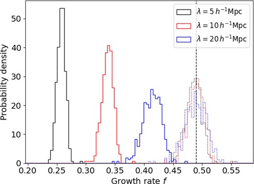
Histograms of best-fitting growth rates to the 400 lognormal realizations, using a velocity–density comparison method, where the model velocity at each point is compared with the measured velocity in the simulation. Results are shown for three different smoothing scales |$\lambda = (5, 10, 20) \, \mathrm{ h}^{-1}$| Mpc. The solid histograms are constructed assuming the model velocity is equal to the reconstructed velocity, and the dotted histograms are constructed after scaling the model velocities in accordance with equation (3). The vertical black dashed line is the fiducial value of the growth rate.
In Appendix A, we detail how this model can be modified in the presence of a survey selection function which modulates the tracer number density field. In future work, we will consider the presence of additional realistic observational effects such as this, together with other factors such as velocity measurement noise and redshift-space distortions.
4 APPLICATION TO DISTANCE INDICATORS
Statistical bias in the reconstructed velocity field will also impact calculations of host galaxy redshifts that are needed to measure H0. The local observed redshift (zobs) of a galaxy used to determine H0 is the product of a cosmic expansion component (zcos) and a contribution from the galaxy peculiar velocity (vpec) in the form
where c is the speed of light.
A single GW event will have the greatest constraining power at low redshift, else the error in H0 will be dominated by the distance error (Chen, Fishbach & Holz 2018; Nicolaou et al. 2020). For nearby sources, however, the impact of peculiar velocities on the observed redshift is more pronounced than for sources at high redshift, where the recessional velocity is much larger by comparison. Uncertainties in the peculiar velocity component can then negatively impact estimates of H0, and if our reconstruction of the velocity field contains statistical or systematic errors we will propagate these errors into our estimates.
Measurements of distance are typically obtained from distance indicators such as standard candles, and an estimate of redshift obtained from accompanying electromagnetic data. GWs offer an alternative approach to estimating cosmic distances that, unlike standard candles, is not dependent on a local distance ladder. Binary inspiral models can be fit to GW signals in order to deduce the physical parameters of the event that produced the wave, and the amplitude of the waveform may be used as a ‘standard siren’ to estimate distance. If there is an electromagnetic counterpart associated with the compact binary coalescence then we may also infer a recessional velocity, and thus directly probe H0 with only a single event (Abbott et al. 2017; Hotokezaka et al. 2019; Nicolaou et al. 2020). GWs do not strictly require a electromagnetic counterpart to be used to estimate H0, and these ‘dark sirens’ can be correlated with galaxy redshift catalogues to localize the signal and predict a host galaxy redshift (Fishbach et al. 2019; Soares-Santos et al. 2019; Finke et al. 2021; Mukherjee et al. 2021a, 2022; Palmese et al. 2023).
Mortlock et al. (2019) present a framework for determining H0 from a sample of GW events with electromagnetic counterparts, which we rewrite as
where the distance to the event is given by D, the cosmological redshift by zcos, and the velocity noise by x, which can represent different combinations of observational and model contributions as we define below.
The uncertainty in the distance measurement, σD, can be written as
where D* is the maximum distance out to which GW sources can be measured by a survey, given some signal-to-noise ratio (SNR) threshold, and σ* = 2D*/SNR is the uncertainty in the distance measurement at D = D*.
We can quantify the error in H0 that we would expect to see as a result of using a biased reconstruction of the local peculiar velocity field, such as that obtained from equations (1) and (2), and compare this with the error in H0 determinations obtained with a corrected velocity field reconstruction, via equation (3). We employ the same set of 400 lognormal realizations as before, each now reduced to a sphere with radius 150 h−1 Mpc centred on an observer and containing on average 1400 objects. Each object in these realizations is associated with three values: the radial distance from the observer – D – in units of h−1 Mpc, the underlying peculiar velocity at the object’s position – u – in units of km s−1, and the model velocity at that position obtained using the linear-theory reconstruction – v – in units of km s−1.
We first convert v into an unbiased prediction of u following equation (3), |$\left(\frac{\sigma _{uv}^2}{\sigma _v^2} \right) v$|, using the previously derived values of σu, σv, and σuv. We further reduce the size of each spherical realization with a distance cut, removing any objects that are within 5 h−1 Mpc of the observer or are beyond some maximum distance set by D*. The cut at the lower bound is made to prevent negative values of H0 upon the addition of randomly sampled observational errors. From this cut catalogue, we then subsample N objects for our ensemble, where N is the number of GW events in our pseudo-catalogue. We calculate the error in the distance for each of these N objects individually by sampling from a normal distribution, where σD is given by equation (10). Assuming a fiducial value of H0 = 70.0 km s−1 Mpc−1, we can also estimate the value of zcos for each object by inverting the Hubble–Lemaitre law, and produce redshift errors for all N objects by sampling from a normal distribution where σz = 10−4. We can then produce a noisy estimate of zcos by adding this redshift error term to the previously estimated value. If the number of objects in the cut catalogue is less than the value of N that we require as a minimum, however, then we do not perform this analysis on that catalogue and move on to the next realization.
We find the best-fitting value of H0 by performing a modified least-squares regression in both the D and z directions, i.e. by minimizing a χ2 function of the form
where |$z_{\rm cos\, ,i}$| and Di are the noisy estimates of the cosmological redshift and distance to the i’th object in the sample, respectively, σz,i and σD,i are their corresponding errors, x is the velocity noise given in equation (9), and σx is the error in this velocity component (see Section 5).
Adopting a maximum-likelihood estimator such as this, rather than explicitly using equation (9) as the estimator for H0, means that we avoid issues caused by dividing through by a noisy measurement such as the distance. Changes in the measurement of the distance caused by noise do not produce symmetric changes in value of |$\hat{H}_0$|. Calculations made with equation (9) are therefore more sensitive to cases where noise reduces our measurement of D, resulting in an overestimate of H0. We show the difference between these approaches in Fig. 5, using both equations to measure the mean value of H0 from the same subsample of objects in each lognormal realization. The maximum-likelihood approach produces results which are centred around the fiducial value of H0 = 70 km s−1 Mpc−1 and are tightly distributed, and we find an average value of H0 = 70.02 ± 0.042 km s−1 Mpc−1. In contrast, results from the ‘ratio’ estimator are more sparsely distributed and are biased towards larger values of H0 than the fiducial value, and we find an average value of H0 = 71.13 ± 0.078 km s−1 Mpc−1. In this example, we have defined the error to be |$\sigma /\sqrt{N}$|, where N = 400 corresponds to the number of lognormal realizations used to produce the H0 measurements. The maximum-likelihood approach also requires the intercept of the fit to pass through the origin, which is an extra constraint not present in the simple estimator approach, driving the improvement in the error.
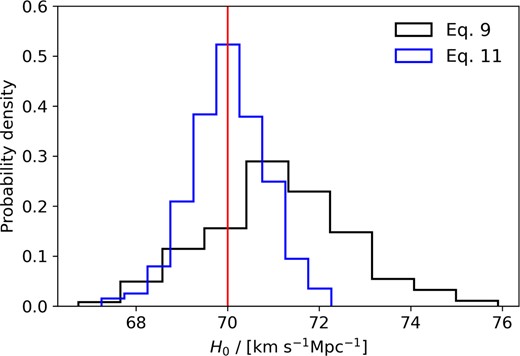
The distribution of the mean values of H0 measured in each of the 400 lognormal mocks, setting D* = 150 h−1 Mpc. The values obtained from the ‘ratio’ estimator equation (9) are shown in blue, and those obtained using the maximum-likelihood estimator equation (11) are shown in black. The red, vertical line represents the fiducial value of H0 = 70 km s−1 Mpc−1.
Performing this fit for each realization, and then taking the mean and standard deviation of the best-fitting values of H0, we verify that we recover H0 in an unbiased manner and also obtain an estimate of the error. We show this process for six randomly selected realizations in Fig. 6, where we subsample each cut catalogue to select N = 50 objects from which we derive a measurement of H0.
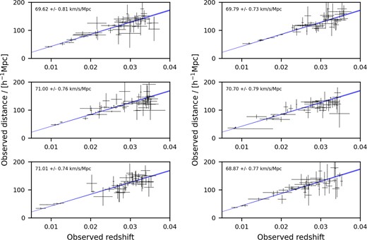
Determinations of H0 obtained from equation (11) for six lognormal realizations selected randomly from our total ensemble of 400. These measurements are made at D* = 150 h−1 Mpc using N = 50 individual objects. The black crosses represent the error in the redshift (on x-axis) and distance (on y-axis) for each of the N objects, and are centred on their measured values (z, D). The blue region represents the ‘measured’ Hubble–Lemaitre law that uses the best-fitting value of H0, and encompasses the 68 per cent confidence interval as defined by the standard deviation. The best-fitting value of H0 and the standard deviation in the measurement obtained from each mock is also given in the top-left corner of their respective panels.
We can compare different reconstructions of the model peculiar velocity field by changing how we consider the velocity noise x, and thus measure how these changes impact the error in estimations of H0. There are three instances of x that we are interested in, specifically. Setting x1 = u is the equivalent of adding a peculiar velocity component to zcos and performing no model velocity correction, thus obtaining zobs = zcos. We can perform a linear-theory model velocity correction by setting x2 = u − v. Finally, we can perform the model correction using the corrected velocity model by setting |$x_3 = u-\left(\frac{\sigma _{uv}^2}{\sigma _v^2} \right) v$|. If the linear-theory model velocity reconstruction is a perfect reflection of the actual local velocity field, then we should recover czcos in case x2. We know this is not the case from Fig. 2, and so instead expect to recover czcos from the corrected model velocity case x3.
By repeating this process for a range of D* values – from 50 to 150 h−1 Mpc in steps of 10 h−1 Mpc – and for all three cases of x described above while keeping N fixed, we can determine how the error in H0 changes with the different model velocity corrections, and as a function of distance. The mean values of H0 for each case, measured using equation (11), are shown in Fig. 7. The shaded regions in Fig. 7 represent the standard deviation across the H0 fits in each D* bin, and are additionally shown in Fig. 8. At the maximum survey distance D* = 150 h−1 Mpc, the error in H0 that we measure for the case x1 is |$\sigma _{H,x_1} = 1.190$| km s−1 Mpc−1, for the case x2 is |$\sigma _{H,x_2} = 0.896$| km s−1 Mpc−1, and for the case x3 is |$\sigma _{H,x_3} = 0.836$| km s−1 Mpc−1.
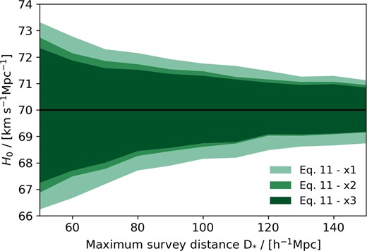
Measurements of H0 made as a function of survey distance D*, obtained by minimizing the χ2 function described by equation (11). The horizontal black line depicts the fiducial value of H0 = 70 km s−1 Mpc−1, while the coloured lines represent the mean values of H0 at each value of D* for each of the three considered model correction cases. The shaded regions depict the standard deviation across the ensemble of H0 measurements about the mean, made at each D*. The colour representing each case is given by the legend in the bottom-right corner.
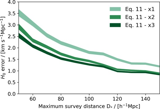
The standard deviation across the set of H0 measurements as a function of D*, the same values are also given in Fig. 7. The shaded region represents the analytical error in the error given by the formula |$\delta \sigma = \sigma /\sqrt{2(N-1)}$|, where N is the number of H0 measurements made in each D* bin. The colour of each region matches that in Fig. 7.
Given the similarity in the errors in Fig. 7, we also present the ‘error in the error’ in Fig. 8 as shaded areas about the standard deviation. We calculate this additional error analytically using the equation |$\delta \sigma = \sigma /\sqrt{2(N-1)}$|, where N is the number of H0 results in each bin.
5 FORECASTS
Mortlock et al. (2019) define the expected uncertainty in a measurement of H0 from a sample of N objects as
where D0, the distance at which σz and σx become unimportant, is
We can therefore compare the measurement errors we obtain in Section 4 to the theoretically ‘ideal’ errors that we should expect from equation (12). For this comparison, we set H0 = 70 km s−1 Mpc−1, D* = 150 h−1 Mpc, N = 50, σz = 10−4, and SNR = 12. The uncertainty in the velocity σx will change depending on the form that our model subtraction x takes, using the three different forms of x discussed in Section 4:
No model subtraction: x1 = u .
Model subtraction: x2 = u − v .
Corrected subtraction: |$x_3 = u-\left(\frac{\sigma _{uv}^2}{\sigma _v^2} \right) v$| .
In the no model correction case, x = u and so we simply recover czcos + u = czobs, while in the two other scenarios we subtract a model velocity component from u in an attempt to recover czcos. We can analytically define the error in the velocity σx for each correction scenario:
No model subtraction: |$\sigma _{x_1}$| = σu = 376 km s−1 .
Model subtraction: |$\sigma _{x_2}$| = |$\sqrt{\sigma _u^2-2\sigma _{uv}^2 + \sigma _v^2}$| = 330 km s−1 .
Corrected subtraction: |$\sigma _{x_3}$| = |$\sqrt{\sigma _u^2-\frac{\sigma _{uv}^4}{\sigma _v^2}}$| = 318 km s−1 .
Here, σu, σv, and σuv are again as previously defined. Thus, we find that the error in the velocity noise σx is minimized when subtracting our new corrected model from the observed redshift. We confirm these results empirically by measuring the standard deviation in the measurements of each definition of x across every object in all 400 lognormal realizations, as well as plotting the distribution in the standard deviations recovered from each realization individually too (see Fig. 9). The values of σx we obtain numerically are all in agreement with the corresponding analytically derived values given above to within |${\lt} 1~{{\ \rm per\ cent}}$|. We can also show that the corrected model subtraction is in fact the optimal choice. Setting x = u − αv, it follows that
If we then vary α such that we minimize σx, we find
confirming the results we obtain in equation (3) and Fig. 9.
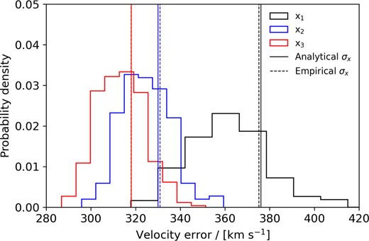
The distribution of velocity errors σx in each treatment of x discussed in Section 4, calculated for each of the 400 lognormal realizations. The case x1 is shown in black, x2 in blue, and x3 in red. The solid vertical lines represent the analytical error for each case, given in Section 5, while the dashed vertical lines represent the numerically derived error when considering every object across all 400 realizations together.
Replacing the value of σx in equation (13) with these three analytically derived quantities, we obtain |$\sigma _{H,x_1} = 1.419$| km s−1 Mpc−1, |$\sigma _{H,x_2} = 1.388$| km s−1 Mpc−1, and |$\sigma _{H,x_3} = 1.380$| km s−1 Mpc−1. We can compare these analytically derived errors to those we obtain empirically from the lognormal realizations, and from the ratio of these two values determine how well our approach in Section 4 works against the forecast measurement error. In the case of applying no model subtraction, x1, the empirical error is |$1.190/1.419 = 0.839 \approx 16~{{\ \rm per\ cent}}$| smaller than the analytical error. Similarly, in the x2 case the empirical error is 35 per cent smaller than the analytical error, and in the x3 case the error is 39 per cent smaller. We summarize this comparison in Table 1.
The H0 error, in units of km s−1 Mpc−1, obtained analytically and empirically using the three values of σx derived in Section 5. For each σx, we also compute the ratio between the analytical and empirical results.
| σx (km s−1) | Forecast σH | Measured σH | Measured/forecast |
|---|---|---|---|
| σx,1 = 376 | 1.419 | 1.190 | 0.839 |
| σx,2 = 330 | 1.388 | 0.896 | 0.646 |
| σx,3 = 318 | 1.380 | 0.836 | 0.606 |
| σx (km s−1) | Forecast σH | Measured σH | Measured/forecast |
|---|---|---|---|
| σx,1 = 376 | 1.419 | 1.190 | 0.839 |
| σx,2 = 330 | 1.388 | 0.896 | 0.646 |
| σx,3 = 318 | 1.380 | 0.836 | 0.606 |
Rather than comparing these errors as analytical against empirical, we can also perform a ‘meta-comparison’, case against case, to see how these methods behave. Analytically, comparing the x3 error to the x1 error we see that |$\sigma _{H,x_3}/\sigma _{H,x_1} = 1.380/1.419 \approx 0.973$| is approximately 2.5 per cent smaller, while empirically we find the error |$\sigma _{H,x_3}/\sigma _{H,x_1} = 0.836/1.190 \approx 0.703$| is approximately 30 per cent smaller. The analytical error in H0 obtained from equation (12) is largely resistant to changes in the value of σx we use, and thus is not sensitive to the choice of model subtraction we apply. The maximum-likelihood method, however, is sensitive to our choice of σx. The error in H0 is much improved when applying any form of model subtraction, biased or otherwise, although the most accurate measurement of H0 is made using the corrected model subtraction.
We are able to significantly improve the uncertainty in our predictions of H0 by making some different choices in constructing our estimator, modifying our model subtraction so that it is optimal, and being mindful to limit the impact of distance errors.
6 CONCLUSIONS
We have introduced a new statistical model for the reconstructed velocity field that minimizes the velocity dispersion when removing the component of observed galaxy redshifts attributable to their peculiar motion. Applying this new model to mock cosmological tests, comparing the measured and model velocity fields to fit for the growth rate of structure, and measuring the current rate of expansion from a sample of GW events, we have shown the potential impact that systematic error in the model velocity field can have when estimating cosmological parameters.
Standard candles and standard sirens captured by next-generation instruments will be used to obtain precision measurements of the Hubble constant in the local Universe. Errors present at low redshift will have a more significant impact on determinations of H0 than the same error at high redshift. We believe it is prescient, then, to ensure that galaxy redshifts properly account for the impact of peculiar velocities on redshift measurements. Commonly applied linear-theory approximations of the velocity field are inherently biased, and do not replicate the mean measured velocity field as we would expect them to. Biases in our reconstructions of the velocity field propagate into cosmological results that are in some way informed by our understanding of the velocity field, most notably the growth rate of structure and the current expansion rate of the Universe. By correcting this discrepancy between the modelled and measured velocity fields, we can mitigate the error in our estimations of cosmological parameters due to galaxy peculiar velocities.
We have explored a framework in which we correct for this bias in the reconstructed velocity field and use the corrected field to estimate the value of H0 for a sample of mock GW events. As part of this framework, we replace the ‘ratio’ estimator with a maximum-likelihood estimator that jointly considers error in the redshift, distance, and velocity observations. Measurements made with the ‘ratio’ estimator are largely influenced by the error in the distance, and by alleviating this we produce a measurement of H0 that is more accurate and unbiased with regard to our fiducial cosmology.
We also compare the errors we obtain numerically with the error expected from analytical forecasts, specifically that set out by Mortlock et al. (2019), which is founded upon the ‘ratio’ estimator equation (9). The errors we obtain are an improvement on this theoretical forecast, and at a maximum survey distance of D* = 150 h−1 Mpc we find that the uncertainty in our estimate of H0 is approximately 39 per cent smaller than predicted by the forecast. In addition, we are able to prove analytically that the correction to the reconstructed velocity field we present is indeed the optimal correction to make, and we also verify this claim empirically.
In our testing of this framework, we have neglected some forms of observational error such as velocity measurement noise and the effect of a survey selection function. Going forward, it will be necessary to apply this corrected velocity model to data sets with more realistic error considerations than our suite of realizations. We also believe that there are implications for BAO reconstruction techniques, and would like to explore the parallels between such techniques and this work in the future.
ACKNOWLEDGEMENTS
We thank the anonymous referee for constructive suggestions that improved the paper. RJT would like to acknowledge the financial support received through a Swinburne University Postgraduate Research Award and Australian Research Council Discovery Project DP220101610.
DATA AVAILABILITY
The data underlying this article will be shared on reasonable request to the corresponding author.
References
APPENDIX A: INCLUDING A SELECTION FUNCTION
We now suppose that the density-field tracer we are using for the velocity-field reconstruction has a non-uniform distribution characterized by a selection function |$W({\boldsymbol{ x}})$|, which is normalized such that |$\sum _{{\boldsymbol{ x}}} W({\boldsymbol{ x}}) = N$|, the total number of tracers. We could infer the overdensity field as |$\delta ({\boldsymbol{ x}}) = N({\boldsymbol{ x}})/W({\boldsymbol{ x}})-1$|, but this approach runs into difficulties when |$W({\boldsymbol{ x}})$| is close to zero. Therefore, analogously to power spectrum estimation (e.g. Feldman, Kaiser & Peacock 1994), we instead adopt a density measure,
where N0 is the average of |$N({\boldsymbol{ x}})$| across the survey volume, and reconstruct the velocity field using |$\delta _N({\boldsymbol{ x}})$| in equation (1). In the presence of a survey selection function, equation (5) is modified to:
where |${\rm Conv} \left(\frac{1}{k^2},|\tilde{W}({\boldsymbol{ k}})|^2 \right)$| denotes the convolution of |$\frac{1}{k^2}$| and the square of the Fourier transform of the window function, |$\tilde{W}({k})$|. This convolution is created by the use of equation (A1) to estimate the density field used in the reconstruction, analogously to the convolution of the model which is the expectation of a power spectrum estimate (Feldman et al. 1994).
As a convenient example to test these methods, we analyse the 600 mock catalogues for the 6-degree Field Galaxy Survey (6dFGS) redshift sample in the redshift range z < 0.1, studied by Turner, Blake & Ruggeri (2023) and originally created by Carter et al. (2018). This selection function extends over the Southern hemisphere for declinations δ < 0°, excluding a region around the Galactic plane, and drops off steeply with increasing redshift owing to the magnitude-limited selection. We ended the selection function in a cuboid of dimensions |$600 \times 600 \times 300 \, \mathrm{ h}^{-1}$| Mpc. We analysed each mock using the methods described in Section 2, and compared the estimated values of the coefficients σu, σv, and σuv from each realization, with the analytical determinations based on equations (4), (6), and (A2). The results are displayed in Fig. A1, indicating that the analytical model provides a good description of the measurements.
![A comparison of the direct measurement of the coefficients of our statistical model relating the reconstructed and measured velocities, σu, σv, and σuv [from which we deduce $r = \sigma _{uv}/(\sigma _u \, \sigma _v)$, with the analytical expressions of equations (4), (6), and (A2)]. We measure the coefficients for 600 6dFGS mock catalogues, and the panels of the figure display their joint distribution (top row), and a histogram (bottom row). The solid red lines indicate the predictions of the analytical model, which are in good agreement with the measurements.](https://oup.silverchair-cdn.com/oup/backfile/Content_public/Journal/mnras/526/1/10.1093_mnras_stad2713/1/m_stad2713figa1.jpeg?Expires=1750218114&Signature=fIVR-tFvM0Urftpv7su-20e16kgEUDZiltCQKRJq49S-sCAwafD2dZnINO9Rs6YX6bawJG1gEaS-NsyzTPKegPl9QtZ3-geBFOml0mpNBun5RUp8vAh8dmGjLjeIzS7Vd3aO~YlJn4ul47WTrQSDRalbXhJPV~EYsN-UDXnOe5Cpv3wcvj4vs7JW-AijqlMOb~DK2-F3cEq7F0MRmWyibrJVyixGGOAX40BNftSSf0gW1GqLFhk8s89w-ySXhHBWXb~muv0Em9VLT2baOryXWHp4VgeQNFlILgGGf2JEwn2p2cRk7iDhDNyqQv5uBNbGsv8eVvPHCBaPLuoqQHAK8Q__&Key-Pair-Id=APKAIE5G5CRDK6RD3PGA)
A comparison of the direct measurement of the coefficients of our statistical model relating the reconstructed and measured velocities, σu, σv, and σuv [from which we deduce |$r = \sigma _{uv}/(\sigma _u \, \sigma _v)$|, with the analytical expressions of equations (4), (6), and (A2)]. We measure the coefficients for 600 6dFGS mock catalogues, and the panels of the figure display their joint distribution (top row), and a histogram (bottom row). The solid red lines indicate the predictions of the analytical model, which are in good agreement with the measurements.
