


ABSTRACT
The |$\rm {H}\alpha$|-to-UV luminosity ratio (|$L(\text{H}\alpha)/L(\rm UV)$|) is often used to probe bursty star formation histories (SFHs) of star-forming galaxies and it is important to validate it against other proxies for burstiness. To address this issue, we present a statistical analysis of the resolved distribution of star formation rate surface density (ΣSFR) as well as stellar age and their correlations with the globally measured |$L(\text{H}\alpha)/L(\rm UV)$| for a sample of 310 star-forming galaxies in two redshift bins of 1.37 < z < 1.70 and 2.09 < z < 2.61 observed by the MOSFIRE Deep Evolution Field (MOSDEF) survey. We use the multiwaveband CANDELS/3D-HST imaging of MOSDEF galaxies to construct ΣSFR and stellar age maps. We analyse the composite rest-frame far-ultraviolet spectra of a subsample of MOSFIRE Deep Evolution Field (MOSDEF) targets obtained by the Keck Low Resolution Imager and Spectrometer (LRIS), which includes 124 star-forming galaxies (MOSDEF-LRIS) at redshifts 1.4 < z < 2.6, to examine the average stellar population properties, and the strength of age-sensitive far-ultraviolet spectral features in bins of |$L(\text{H}\alpha)/L(\rm UV)$|. Our results show no significant evidence that individual galaxies with higher |$L(\text{H}\alpha)/L(\rm UV)$| are undergoing a burst of star formation based on the resolved distribution of ΣSFR of individual star-forming galaxies. We segregate the sample into subsets with low and high |$L(\text{H}\alpha)/L(\rm UV)$|. The high-|$L(\text{H}\alpha)/L(\rm UV)$| subset exhibits, on average, an age of |$\log [\rm {Age/yr}]$| = 8.0, compared to |$\log [\rm {Age/yr}]$| = 8.4 for the low-|$L(\text{H}\alpha)/L(\rm UV)$| galaxies, though the difference in age is significant at only the 2σ level. Furthermore, we find no variation in the strengths of Si iv λλ1393, 1402 and C iv λλ1548, 1550 P-Cygni features from massive stars between the two subsamples, suggesting that the high-|$L(\text{H}\alpha)/L(\rm UV)$| galaxies are not preferentially undergoing a burst compared to galaxies with lower |$L(\text{H}\alpha)/L(\rm UV)$|. On the other hand, we find that the high-|$L(\text{H}\alpha)/L(\rm UV)$| galaxies exhibit, on average, more intense He ii λ1640 emission, which may possibly suggest the presence of a higher abundance of high-mass X-ray binaries.
1 INTRODUCTION
While most galaxies follow a tight sequence in star formation rate (SFR) versus stellar mass (M*), there are some that are significantly offset above this relation at any given redshift, suggestive of a recent burst of star formation (Schmidt 1959; Kennicutt 1989; Somerville & Primack 1999; Springel 2000; Springel, Di Matteo & Hernquist 2005; Noeske et al. 2007; Dobbs & Pringle 2009; Kereš et al. 2009; Knapen & James 2009; Genzel et al. 2010; Governato et al. 2010; Reddy et al. 2012; Hopkins et al. 2014; Rodighiero et al. 2014; Shivaei et al. 2015; Hayward & Hopkins 2017; Fujimoto et al. 2019; Wang & Lilly 2020). For example, the apparent increase in scatter of the relationship between SFR and M* at low stellar masses suggests that such galaxies are characterized by bursty star formation histories (SFHs; Noeske et al. 2007; Hopkins et al. 2014; Shen et al. 2014; Guo et al. 2016; Asquith et al. 2018; Dickey et al. 2021; Atek et al. 2022). In addition, simulations with resolved scaling comparable to the star-forming clouds suggest that the burst amplitude and frequency increase with redshift (e.g. Feldmann et al. 2017; Sparre et al. 2017; Ma et al. 2018). Given that bursty SFHs are inferred to be the likely mode of galaxy growth for at least lower mass galaxies at high redshift (e.g. Atek et al. 2022 found evidence of bursty SFHs for lower mass galaxies with |$M_{\ast }\lt 10^{9}\, {\rm M}_{\odot }$| at z ∼ 1.1), it is important to determine the effectiveness of commonly used proxies for burstiness.
A key method that has been used to infer the burstiness1 of star-forming galaxies is to compare SFR indicators that are sensitive to star formation on different time-scales. Two of the widely used SFR indicators are derived from the H α nebular recombination line (|$\lambda = 6564.60\, {\mathring{\rm A}}$|) and far-ultraviolet (FUV) continuum (|$1300\, {\mathring{\rm A}}\lt \lambda \lt 2000\, {\mathring{\rm A}}$|). The H α emission line originates from the recombination of the ionized gas around young massive stars (|$M_{\ast }\gtrsim 20\,{\rm M}_{\odot }$|) and traces SFR over a time-scales of ∼10 Myr (Kennicutt & Evans 2012). The UV continuum is sensitive to the same stars that are responsible for H α, as well as lower mass stars (B stars, and A stars at wavelengths redder than 1700 |$\mathring{\rm A}$|) with lifetimes of ∼100 Myr and |$M_{\ast }\gtrsim \, 3\,{\rm M}_{\odot }$|. As a result, when compared to the H α emission line, the FUV continuum traces SFRs averaged over a longer time-scale. Therefore, variations in the dust-corrected H α-to-UV luminosity ratio (|$L(\rm{H\alpha })/L(\rm UV)$|) may reveal information about recent burst activity (Glazebrook et al. 1999; Iglesias-Páramo et al. 2004; Lee et al. 2009, 2011; Meurer et al. 2009; Hunter, Elmegreen & Ludka 2010; Fumagalli, da Silva & Krumholz 2011; da Silva, Fumagalli & Krumholz 2012, 2014; Weisz et al. 2012; Domínguez et al. 2015; Caplar & Tacchella 2019; Emami et al. 2019; Faisst et al. 2019).
For a constant SFH, the H α-to-UV luminosity ratio will reach to its equilibrium after a few tens of Myr (e.g. Reddy et al. 2012). However, variations in the inferred integrated H α-to-UV ratio may result from a number of effects, including variations in the initial mass function (IMF) (Leitherer & Heckman 1995; Elmegreen 2006; Pflamm-Altenburg, Weidner & Kroupa 2007; Hoversten & Glazebrook 2008; Boselli et al. 2009; Meurer et al. 2009; Pflamm-Altenburg, Weidner & Kroupa 2009; Mas-Ribas, Dijkstra & Forero-Romero 2016), nebular and stellar dust reddening (Kewley et al. 2002; Lee et al. 2009; Reddy et al. 2012, 2015; Shivaei et al. 2015, 2018; Theios et al. 2019), ionizing escape fraction (Steidel, Pettini & Adelberger 2001; Shapley et al. 2006; Siana et al. 2007), and binary stellar evolution (Eldridge 2012; Choi, Conroy & Byler 2017; Eldridge et al. 2017). In addition, comparing the mock Hubble Space Telescope (HST) and James Webb Space Telescope (JWST) galaxy catalogues with 3D-HST observations of z ∼ 1 galaxies, Broussard et al. (2019) find that the average H α-to-UV ratio is not impacted significantly by variations in the high-mass slope of the IMF, and metallicity. Similar studies also show that the average H α-to-UV is not a good indicator of business but rather a probe of the average SFH or dust law uncertainties (Broussard et al. 2019; Broussard, Gawiser & Iyer 2022). Given these possibilities, any interpretation about the burstiness of galaxies based on the variations in |$L(\rm{H\alpha })/L(\rm UV)$| must be approached with caution.
The MOSFIRE Deep Evolution Field (MOSDEF) survey is ideally suited to examine the extent to which variations in |$L(\rm{H\alpha })/L(\rm UV)$| trace burstiness. MOSDEF probes galaxies at z ∼ 2, which marks a key epoch for galaxy growth when the cosmic star formation density reaches its maximum (Madau et al. 1996; Hopkins & Beacom 2006; Madau & Dickinson 2014). Additionally, the deep HST imaging of the MOSDEF galaxies obtained by CANDELS (Grogin et al. 2011; Koekemoer et al. 2011) enables the construction of stellar population maps that can be used to assess burstiness on smaller (resolved) spatial scales (e.g. Wuyts et al. 2011, 2012; Hemmati et al. 2014; Jafariyazani et al. 2019; Fetherolf et al. 2020). Moreover, the availability of follow-up Keck/Low Resolution Imager and Spectrometer (LRIS) rest-FUV spectra of a subset of 259 MOSDEF galaxies (Topping et al. 2020; Reddy et al. 2022) allows us to investigate the relationship between the |$L(\rm{H\alpha })/L(\rm UV)$| ratio and age-sensitive FUV spectral features.
The goal of this study is to determine whether the dust-corrected H α-to-UV luminosity ratio is a reliable tracer of a bursty SFH at z ∼ 2. We address this question by examining the correlations between the differences in properties of the stellar populations and the |$L(\rm{H\alpha })/L(\rm UV)$| ratio. The structure of this paper is as follows. In Section 2, we introduce the samples used in this work, and outline the sample selection criteria and data reduction. In Section 3, we describe the method used for constructing the stellar population maps, and the result of the morphology analysis. Our approach for constructing rest-FUV composite spectra is described in Section 4. Our results on variations of the average physical properties of galaxies, and the strength of age-sensitive FUV spectral features in bins of |$L(\rm{H\alpha })/L(\rm {UV})$| are presented in Section 5. Finally, the conclusions are summarized in Section 6. Wavelengths are in the vacuum frame. We adopt a flat cosmology with |$H_{0}=70\, \rm {km \, s^{-1}}$|, ΩΛ = 0.7, and Ωm = 0.3. A Chabrier (2003) IMF is assumed throughout this work.
2 SAMPLE
2.1 Rest-frame optical MOSDEF spectroscopy
The MOSDEF survey (Kriek et al. 2015) used the Keck/MOSFIRE spectrograph (McLean et al. 2012) to obtain rest-frame optical spectra of |$\sim 1500\, H$|-band-selected star-forming galaxies and active galactic nuclei (AGNs). The five extragalactic legacy fields (GOODS-S, GOODS-N, COSMOS, UDS, AEGIS) covered by the CANDELS survey (Grogin et al. 2011; Koekemoer et al. 2011) were targeted. The targets were chosen to lie in three redshift bins: 1.37 < z < 1.70, 2.09 < z < 2.61, and 2.95 < z < 3.80 where the strong rest-frame optical emission lines (|$\rm{[O\,{\small II}]}\lambda 3727,3730$|, H β, |$\rm{[O\,{\small III}]}\lambda \lambda 4960,5008$|, H α, |$\rm{[N\,{\small II}]}\lambda \lambda 6550,6585$|, and |$\rm{[S\,{\small II}]}\lambda 6718,6733$|) are redshifted into the YJH, JHK, and HK transmission windows, respectively. Further details of the survey and MOSFIRE spectroscopic data reduction are provided in Kriek et al. (2015).
We use the spectroscopic redshifts and emission lines measured by the MOSDEF survey. The spectroscopic redshift for each target was measured from the observed wavelength centroid of the highest signal-to-noise emission line in each spectrum. Emission-line fluxes were measured from the 1D-spectra of the individual objects by fitting Gaussian functions along with a linear continuum. The H α was fit simultaneously with the |$\rm{[N\,{\small II}]}$| doublet using three Gaussian functions. The H α emission line flux was corrected for the underlying Balmer absorption, which was measured from the best-fitting stellar population model (Section 2.4). Line flux uncertainties were calculated by perturbing the observed spectra according to their error spectra and remeasuring the line fluxes 1000 times. The 68th percentile of the distribution obtained from these iterations was adopted to represent the upper and lower flux uncertainties (e.g. Reddy et al. 2015; William et al. 2019).
2.2 CANDELS/3D-HST Imaging
Resolved broad-band photometry of the MOSDEF galaxies was obtained by CANDELS using HST/ACS in the F435W (B435), F606W (V606), F775W (i775), F813W (I814), and F850LP (z850) filters and HST/WFC3 in the F125W (J125), F140W (JH140), and F160W (H160) filters. CANDELS imaging covered |$\sim 960\,$| arcmin2 up to a 90 per cent completeness in the H160 filter at a magnitude of |$25\,$|mag. To construct stellar population maps for the sample galaxies, we use the processed CANDELS images provided by the 3D-HST grism survey team (Brammer et al. 2012; Skelton et al. 2014; Momcheva et al. 2016) along with the publicly available2 photometric catalogues with coverage from 0.3 to |$0.8\, \mu$|m. The HST images provided by the 3D/HST team were drizzled to a |$0.06\,$|arcsec pixel−1 scale and smoothed to produce the same spatial resolution as the H160 images (|$0.18\,$|arcsec).
The final sample used in this work contains 310 typical star-forming galaxies at 1.36 < z < 2.66, all meeting the following criteria. They all have spectroscopic redshifts from the MOSDEF survey and detections of H α and H β emission lines with S/N ≥ 3. AGNs were identified and excluded from the sample based on the IR properties, X-ray luminosities, or [N ii]λ6584/H α line ratio criteria as described in Coil et al. (2015), Azadi et al. (2017, 2018), and Leung et al. (2019). Additional S/N and resolution constraints were applied to the HST photometry as a result of our approach of grouping pixels which will be discussed in Section 3.
The final sample described above is used to analyse the morphological information of the MOSDEF galaxies in the first part of this work (i.e. Section 3), and is referred to as the MOSDEF/MORPH sample throughout this work. This sample is based on that used by Fetherolf et al. (2023). The MOSDEF/MORPH sample covers a range of stellar mass of 8.77 < log [M*/M⊙] < 11.04, and a SFR[H α] range of |$0.40\lt (\text{SFR[H$\alpha $]}/{\rm M}_{\odot }\rm {yr}^{-1})\lt 130$|. As shown in the middle panel of Fig. 1, the MOSDEF/MORPH sample galaxies lie systematically above the mean main-sequence relation found by Shivaei et al. (2015) based on the first 2 yr of MOSDEF. This is due to the S/N and resolution criteria (Section 3) imposed on the HST photometry of MOSDEF galaxies. Using these requirements results in a sample that is biased against low-mass and compact galaxies (Fetherolf et al. 2020). The S/N requirement for H β emission line is necessary to obtain a more reliable Balmer decrement measurement for each galaxy and does not introduce a significant bias in the sample (Reddy et al. 2015; Shivaei et al. 2015; Sanders et al. 2018; Fetherolf et al. 2021). As evidenced in the middle panel of Fig. 1, our sample galaxies do not display any substantial bias relative to the mean main-sequence relation determined by Shivaei et al. (2015), which was derived irrespective of H β detection. The MOSDEF/MORPH sample galaxies exhibit a similar range of |$L(\rm{H\alpha })/L(\rm {UV})$| to the MOSDEF parent sample galaxies that have coverage of H α and H β with significant detections (S/N ≥ 3) and include galaxies with |$L(\rm{H\alpha })/L(\rm {UV})$| that lie at least 5σ below the mean ratio for the MOSDEF parent sample. The S/N requirement for H β emission does not significantly impact the average |$L(\rm{H\alpha })/L(\rm UV)$| ratio. If we consider those galaxies where H β is not detected at the S/N ≥ 3 but still covered in the spectra, the average |$L(\rm{H\alpha })/L(\rm UV)$| decreases by approximately 31 per cent, which falls within the measurement uncertainty when considering the S/N ≥ 3 requirement. Regardless of the H β detection requirement, the average |$L(\rm{H\alpha })/L(\rm UV)$| values and the asymptotic |$L(\rm{H\alpha })/L(\rm UV)$| are consistent within the measurement uncertainties. As mentioned earlier in this section, L(H α) used here is obtained by the MOSDEF survey, and is corrected for the effect of dust using an MW extinction curve (Cardelli, Clayton & Mathis 1989) which is shown to best represent the nebular attenuation curve for both high-redshift and local galaxies (Reddy et al. 2020; Rezaee et al. 2021). UV luminosity (|$L(\rm UV)$|) is estimated by using the best-fitting SED models at |$\lambda =1500\, {\mathring{\rm A}}$|. A more detailed discussion on calculating the dust-corrected |$L(\rm UV)$| is presented in Section 2.4.
![Physical properties of 310 star-forming galaxies in the MOSDEF/MORPH sample used in this work. Left panel: The histogram indicates the MOSDEF spectroscopic redshift distribution in two bins with the average redshifts of z ∼ 1.5 and ∼2.3. Middle panel: SFR[H α] versus M* relationship. SFR[H α] is computed using the dust-corrected H α luminosity. The conversion factor between the H α luminosity and SFR[H α], as well as stellar mass are derived using the SED modeling. The dashed red line shows Shivaei et al. (2015) relationship between SFR[H α] and M*, which has been adjusted to represent the assumptions used in this work, based on the first 2 yr of MOSDEF (including galaxies with undetected Hβ). The horizontal dashed lines represent the 3σ detection limits of the SFR[H α] determined for the two redshift bins (1.37 < z < 1.70, and 2.09 < z < 2.61) using H- and K-band line sensitivities (Kriek et al. 2015). Right panel: The distribution of dust-corrected $L(\rm{H\alpha })/L(\rm UV)$ with respect to the stellar mass where L(H α) and $L(\rm {UV})$ are dust-corrected using the Cardelli et al. (1989) and SMC extinction curves, respectively. The red-dashed line indicates the average dust-corrected $L(\rm{H\alpha })/L(\rm UV)$ of all the galaxies in the MOSDEF parent sample that have coverage of H α and H β emission lines with S/N ≥ 3. The green dashed line indicates the asymptotic value of $L(\rm{H\alpha })/L(\rm UV)$ for a constant SFH using BPASS SED models (Section 2.4).](https://oup.silverchair-cdn.com/oup/backfile/Content_public/Journal/mnras/526/1/10.1093_mnras_stad2842/1/m_stad2842fig1.jpeg?Expires=1749175347&Signature=rytvk6Du1a4fZLNLPEf1CkSiJcvK6zhONFHv83JABCgZQT~fZzq5xg69s3HBhwWxwNnIL5PU3v2CeiCGDVytvhqFgaOgpmnEoHE~IwO~FIUO2VIrMtCj1WoxKCphg6vmv126TkHgslek08~90e7JCpL1fuRFDBvHo3kuXH-vpN8YV51pLt9RH~0z40pCoH4xsfMXmjIrVsRnRoF-KRYS2n6qyXFeEbRW7TTnXfzUU1KK9Oze-4BOgLjXzKJ0tji84B2BTMx0LBmrUylZsX1P7cYJoD9ax6TI8J7hf2HStFQX5PUP6OC9-xu75CoOyqggxbh1DZ4SYroGOMSkv~rFZA__&Key-Pair-Id=APKAIE5G5CRDK6RD3PGA)
Physical properties of 310 star-forming galaxies in the MOSDEF/MORPH sample used in this work. Left panel: The histogram indicates the MOSDEF spectroscopic redshift distribution in two bins with the average redshifts of z ∼ 1.5 and ∼2.3. Middle panel: SFR[H α] versus M* relationship. SFR[H α] is computed using the dust-corrected H α luminosity. The conversion factor between the H α luminosity and SFR[H α], as well as stellar mass are derived using the SED modeling. The dashed red line shows Shivaei et al. (2015) relationship between SFR[H α] and M*, which has been adjusted to represent the assumptions used in this work, based on the first 2 yr of MOSDEF (including galaxies with undetected Hβ). The horizontal dashed lines represent the 3σ detection limits of the SFR[H α] determined for the two redshift bins (1.37 < z < 1.70, and 2.09 < z < 2.61) using H- and K-band line sensitivities (Kriek et al. 2015). Right panel: The distribution of dust-corrected |$L(\rm{H\alpha })/L(\rm UV)$| with respect to the stellar mass where L(H α) and |$L(\rm {UV})$| are dust-corrected using the Cardelli et al. (1989) and SMC extinction curves, respectively. The red-dashed line indicates the average dust-corrected |$L(\rm{H\alpha })/L(\rm UV)$| of all the galaxies in the MOSDEF parent sample that have coverage of H α and H β emission lines with S/N ≥ 3. The green dashed line indicates the asymptotic value of |$L(\rm{H\alpha })/L(\rm UV)$| for a constant SFH using BPASS SED models (Section 2.4).
2.3 MOSDEF/LRIS rest-FUV spectroscopy
A subset of 259 objects from the MOSDEF parent sample were selected for deep rest-FUV spectroscopic follow-up observations with the Keck I/LRIS (Oke et al. 1995; Steidel et al. 2004). We refer the reader to Topping et al. (2020) and Reddy et al. (2022) for further details about the MOSDEF/LRIS survey data collection and reduction procedures. In brief, targets were prioritized based on S/N ≥ 3 detection of the four emission lines ([O iii], H β, [N ii]λ6584, and H α) measured by the MOSDEF survey. Objects with available H α, H β, and [O iii] as well as an upper limit on [N ii] were accorded the next highest priority. The objects with available spectroscopic redshifts from the MOSDEF survey, as well as those without secure redshift measurements, were also included. The lowest priority was assigned to the objects that were not included in the MOSDEF survey, but had photometric redshifts and apparent magnitudes from the 3D-HST catalogues that were within the MOSDEF survey redshift ranges.
Rest-FUV LRIS spectra were obtained within nine multiobject slit masks with 1|${_{.}^{\prime\prime}}$|2 slits in four extragalactic legacy fields: GOODS-S, GOODS-N, AEGIS, and COSMOS. The d500 dichroic was used to split the incoming beam at |$\simeq 5000\, {\mathring{\rm A}}$| were used to obtain the LRIS spectra. The blue and red-side channels of LRIS were observed with the 400 line mm–1 grism blazed at |$4300 \ {\mathring{\rm A}}$|, and the 600 line mm–1 grating blazed at |$5000 \ {\mathring{\rm A}}$|, respectively. This configuration yielded a continuous wavelength range from the atmospheric cutoff at |$3100\, {\mathring{\rm A}}$| to |$\sim 7650\, {\mathring{\rm A}}$| (the red wavelength cutoff depends on the location of the slit in the spectroscopic field of view) with a resolution of R ∼ 800 on the blue side and R ∼ 1300 on the red side. The final MOSDEF/LRIS sample used in the second part of this work (i.e. Section 5) includes 124 star-forming galaxies at 1.42 < z < 2.58, all meeting the same S/N and redshift measurement requirements as those mentioned in Section 2.1.
2.4 SED modelling
We use the Binary Population and Spectral Synthesis (BPASS) version 2.2.1 models3 (Eldridge et al. 2017; Stanway & Eldridge 2018) to infer UV luminosity (|$L(\rm UV)$|), stellar continuum reddening (E(B − V)cont), stellar ages, conversion factors between luminosities and SFRs, as well as stellar masses (M*). The effect of binary stellar evolution is included in the BPASS SED models, which has been found to be an important assumption in modelling the spectra of high-redshift galaxies (Steidel et al. 2016; Eldridge et al. 2017; Reddy et al. 2022). These models are characterized by three sets of parameters, stellar metallicity (Z*) ranging from 10−5 to 0.040 in terms of mass fraction of metals where solar metallicity (Z⊙) is equal to 0.0142 (Asplund et al. 2009), the upper-mass cutoff of the IMF (Mcutoff = {100 M⊙, 300 M⊙}), and the choice of including binary stellar evolution. These parameters divide the models into four sets of model assumptions with various Mcutoff and whether or not the binary effects are included. Throughout, we refer to these model combinations as ‘100bin’, ‘300bin’, ‘100sin’, and ‘300sin’ where the initial number indicate the Mcutoff of the IMF and ‘bin’ (‘sin’) indicates that the binary evolution is (or is not) included (Reddy et al. 2022).
Stellar population synthesis (SPS) models are constructed by adding the original instantaneous-burst BPASS models for ages ranging from |$10^{7}\,$|-|$10^{10}\,$| yr while adopting a constant SFH.4 The choice of constant SFH over instantaneous burst models is based on the fact that the latter are better suited for the individual massive star clusters that are more age-sensitive than the entire high-redshift star-forming galaxies, which have dynamical times that are typically far greater than a few Myr (Papovich, Dickinson & Ferguson 2001; Shapley et al. 2001; Reddy et al. 2012). The reddening of the stellar continuum is added to the models assuming the following attenuation curves: the SMC (Gordon et al. 2003), Reddy et al. (2015), and Calzetti et al. (2000), with stellar continuum reddening in range of E(B − V)cont = 0.0−0.60. Based on earlier studies, these curves are shown to best represent the shape of the dust attenuation curves for the majority of high-redshift galaxies (e.g. Reddy et al. 2018; Fudamoto et al. 2020; Shivaei et al. 2020).
When fitting the broad-band photometry, the stellar metallicity is held fixed at |$\langle$|Z*〉 =0.001 as this value was found to best fit the rest-FUV spectra of galaxies in the MOSDEF/LRIS sample (Topping et al. 2020; Reddy et al. 2022). The stellar population ages of the models are permitted to range between |$\sim 10\,$| Myr and the age of the universe at the redshift of each galaxy. Unless mentioned otherwise, the BPASS model with binary stellar evolution, an upper-mass cutoff of |$100\, {\rm M}_{\odot }$| (‘100bin’), and the SMC extinction curve are adopted for this analysis. Previous studies (e.g. Reddy et al. 2022) have shown that using the SMC dust attenuation curve results in better agreement between H α and SED-derived SFRs. Assuming the Z* = 0.001, 100 bin BPASS SPS models in fitting the broad-band photometry yields a conversion factor of |$2.12 \times 10^{-42}\, {\rm M}_{\odot } \rm {yr}^{-1} \rm {erg}^{-1} s$| between the dust-corrected H α luminosity and SFR[H α]. The dust-corrected |$L(\rm UV)$| is determined using the best-fitting model at |$\lambda =1500\, {\mathring{\rm A}}$| and the best-fitting stellar continuum reddening.
The best-fitting SED model is chosen by fitting the aforementioned models to broad-band photometry. The parameters of the model with the lowest χ2 relative to the photometry are considered to be the best-fitting values. The errors in the parameters are calculated by fitting the models to many perturbed realizations of the photometry according to the photometric errors. The resulting standard deviations in the best-fitting model values give the uncertainties in these values.
3 MORPHOLOGY ANALYSIS
In this section, we present a methodology to construct resolved stellar population maps that may unveil galaxies undergoing bursts of star formation on smaller (∼10 kpc) spatial scales. We also examine the correlation between the resolved stellar population properties and |$L(\rm{H\alpha })/L(\rm {UV})$|.
3.1 Pixel Binning
Rather than studying the individual images pixel by pixel, we group pixels using the two-dimensional Voronoi binning technique introduced by Cappellari & Copin (2003) and further modified by Fetherolf et al. (2020). The point spread function of the CANDELS imaging is larger than the individual pixels (0|${_{.}^{\prime\prime}}$|18), such that we apply a Voronoi binning technique to the imaging in order to avoid correlated noise between individual analyzed elements. In brief, each of the 3D-HST images (Section 2.2) is divided into sub-images 80 pixels on a side. We use the SExtractor (Bertin & Arnouts 1996) segmentation map to mask pixels in each sub-image that are not associated with the galaxy. The pixels are grouped following the algorithm presented in Cappellari & Copin (2003) to attain S/N ≥ 5 in at least five different filters (see e.g. Fetherolf et al. 2020). Alongside CANDELS imaging, we use unresolved Spitzer/IRAC photometry to cover the rest-frame near-infrared part of the spectrum. As the HST and Spitzer/IRAC photometry have different spatial resolutions, we assign IRAC fluxes to each of the Voronoi bins proportionally according to the H160 flux (see Fetherolf et al. 2020 for further details). The stellar population properties for each Voronoi bin are inferred using the SED models (see Section 2.4) that best fit the resolved 3D-HST photometry (Wuyts et al. 2011, 2012, 2013; Hemmati et al. 2014; Lang et al. 2014). We calculate SFR surface density (ΣSFR[SED]) for each Voronoi bin by dividing the SFR determined from the best-fitting resolved SED model by the area of each Voronoi bin. Fig. 2 shows examples of the Voronoi bins and stellar population maps for two galaxies in the sample, one in each targeted redshift range.
![Examples of SFR surface density (ΣSFR[SED]) maps using Voronoi bins. The field name and 3D-HST Version 4.0 ID of each galaxy, as well as their redshifts, are indicated in the top left corner of each panel.](https://oup.silverchair-cdn.com/oup/backfile/Content_public/Journal/mnras/526/1/10.1093_mnras_stad2842/1/m_stad2842fig2.jpeg?Expires=1749175347&Signature=mG4nQxyX5E0PFSrdwE5XBKABAyynQpk4N9HXSNiEcIkgQnEUhNE2NFUMEVAl1wOC5HTbgfSrq~sqXiz1Ht5wfgWVe2zXANVek4JNa9RwEEd2X8OTq1HX754knaHnYprjNyHavD6UAqPRLO2MT6F4Gi5mtOMctpK2MuGI8Pfan46KuLCrovuxeaRY1KWshFO4h20vIAzs~K7f8F49IvrleOPDxp3TudGf7DRJvAjEqu0Yh~NobJm88cRDf-QXNhdkYzsD5JM6cQ8pkiwA9s6MOq66dwFGozmrxhbXcYpIUW5aFXqAk4PdWKzBkqKZRYtxYX~C~EOylApm44wZMKk~rg__&Key-Pair-Id=APKAIE5G5CRDK6RD3PGA)
Examples of SFR surface density (ΣSFR[SED]) maps using Voronoi bins. The field name and 3D-HST Version 4.0 ID of each galaxy, as well as their redshifts, are indicated in the top left corner of each panel.
3.2 Patchiness
Patchiness (P) is a recently introduced morphology metric (Fetherolf et al. 2023) that evaluates the Gaussian likelihood that each of the distinct components of a distribution is equal to the weighted average of the distribution. In this analysis, individual elements are values of a parameter measured for each of the resolved Voronoi bins. The area-weighted average of the parameter X measured from individual Voronoi bins is defined by
where Xi are the values measured for the parameter X inside each of the Voronoi bins with uncertainty σi, Nbins is the total number of Vornoi bins in a galaxy photometry, and npix is the total number of pixels inside a single Voronoi bin (area). The patchiness, P(X), can be calculate by equation (2) in Fetherolf et al. (2023) as
A detailed discussion and evaluation of the patchiness metric properties are presented in Fetherolf et al. (2023). In brief, patchiness can be compared most reliably between galaxies with similar redshifts. Thus, we divide galaxies into two bins of redshift and analyse the patchiness separately for galaxies in each bin. Moreover, patchiness can be used on parameters with large dynamic ranges or parameters with values close to zero. We study patchiness of ΣSFR[SED] which traces the concentration of star formation within the Voronoi bins, and exhibits a large dynamic range among our sample galaxies. A single Voronoi bin has, on average, a size of |$\sim 4.5\, \rm {kpc^{2}}$|, and a median size of |$\sim 1.5\, \rm {kpc^{2}}$|. The estimated typical dynamical time-scale for a Voronoi bin is |$\sim 10\,$| Myr, based on the velocity dispersion assumption inferred from studies on z ∼ 2 galaxies with comparable size measurements to the Voronoi bins used in this work (Erb et al. 2006; Law et al. 2009, 2012; Reddy et al. 2012; Fetherolf et al. 2020). A physical example of how patchiness can be used is presented in Fetherolf et al. (2023), where higher patchiness values of stellar reddening indicate a more complex dust distribution.
A burst of star formation on top of an underlying constant SFH can result in an increase in ΣSFR. An element of a resolved population containing a burst of star formation has a higher ΣSFR and a younger stellar age compared to other elements, resulting in a larger P(ΣSFR[SED]), and |$P(\rm {Age})$|. Therefore, large P(ΣSFR[SED]) may suggest the presence of bursts in localized (Voronoi) regions of galaxies. Fig. 3 indicates the relationship between the stellar age and ΣSFR[SED] derived for Voronoi bins constructed for all the galaxies in the MOSDEF/MORPH sample. The figure indicates that younger stellar populations are found in regions with higher SFR surface densities.
![SFR surface density versus stellar age of Voronoi bins constructed for all the galaxies in the MOSDEF/MORPH sample (grey). Average values of ΣSFR[SED] in bins of stellar age $\log [\rm Age/yr]$ are shown by the blue stars. A total of 26 Voronoi bins are estimated at a stellar age of $10^{8}\,$ yr, with 12 bins exhibiting ΣSFR[SED] ≥ 0.1, accounting for the noticeable outlier.](https://oup.silverchair-cdn.com/oup/backfile/Content_public/Journal/mnras/526/1/10.1093_mnras_stad2842/1/m_stad2842fig3.jpeg?Expires=1749175347&Signature=yH2ram71wCXrrtGErhmmNEUMehKYTwn13wGJw~2qAwHIhHh4ceJxHnvKNQXoMMJPBBGenIEMIARuPPaZfbzOj5VV~TXkTyERG7Wf51dvVXz-bnM9Ebf6BvJJnq-2l~L0cAUXXgIUNZ8-VFlnU8zVpX143n3vtqMaacvuoUcCiqKg9YBeKVuddv86ffZN4wg4ZNCzHsnlKKvO-2NLfS843-ycOaPZ0mJljO2aZ9nq7LdxwmlDqaes-96nSSwgY5U61Czlt8XFGzSDNtBQgI4DBtsfAxwhxoHo1KGwInca9Dk6daAQx4QHZMuHyoh-SrsS68pNJdMFYha0iVCt4QZN9A__&Key-Pair-Id=APKAIE5G5CRDK6RD3PGA)
SFR surface density versus stellar age of Voronoi bins constructed for all the galaxies in the MOSDEF/MORPH sample (grey). Average values of ΣSFR[SED] in bins of stellar age |$\log [\rm Age/yr]$| are shown by the blue stars. A total of 26 Voronoi bins are estimated at a stellar age of |$10^{8}\,$| yr, with 12 bins exhibiting ΣSFR[SED] ≥ 0.1, accounting for the noticeable outlier.
3.3 Patchiness of ΣSFR[SED] versus |$L(\rm{H\alpha })/L(\rm UV)$|
This section presents our results on the correlation between P(ΣSFR[SED]) and |$L(\rm{H\alpha })/L(\rm UV)$|. Given that star formation mode varies in strength, duration, or a combination of both factors in different regions of a galaxy (Reddy et al. 2012; Dale et al. 2016, 2020; Smith et al. 2021), and patchiness is sensitive to outliers below and above the average, we expect P(ΣSFR[SED]) to be large for galaxies that are undergoing a burst of star formation that could be detected on resolved scales.
Due to surface brightness dimming, higher redshift objects, on average, have fewer and larger Voronoi bins. To control for this effect, we divide the MOSDEF sample into two subsamples in the redshift ranges of 1.37 < z < 1.70 (z ∼ 1.5) and 2.09 < z < 2.61 (z ∼ 2.3). Fig. 4 shows the relationship between P(ΣSFR[SED]) and |$L(\rm{H\alpha })/L(\rm UV)$| for galaxies in each redshift bin. Based on a Spearman correlation test, we find no significant correlation between the two for both the z ∼1.5 and 2.3 subsamples, with probabilities of Pn = 0.30 and 0.36, respectively, of a null correlation. As shown by the stellar age colour-coded points, a higher P(ΣSFR[SED]) corresponds to a higher |$P(\rm Age)$|, which is expected given that stellar age and SFR surface density are correlated for a given SPS model. There is also a lack of correlation between |$L(\rm{H\alpha })/L(\rm UV)$| and |$P(\rm Age)$| with correlation properties reported in Table 1.
![The MOSDEF/MORPH sample: P(ΣSFR[SED]) versus dust-corrected $L(\rm{H\alpha })/L(\rm UV)$ for two redshift bins centred at z ∼ 1.5 (left panel) and z ∼ 2.3 (right panel). The points are coloured by patchiness of the stellar age. No significant correlations are found between $L(\rm{H\alpha })/L(\rm UV)$ and P(ΣSFR[SED]), or between $L(\rm{H\alpha })/L(\rm UV)$ and $P(\rm Age)$. The Spearman correlation properties for the relations shown in this figure are reported in Table 1.](https://oup.silverchair-cdn.com/oup/backfile/Content_public/Journal/mnras/526/1/10.1093_mnras_stad2842/1/m_stad2842fig4.jpeg?Expires=1749175347&Signature=n8XcNK3CFe1CwX275whGqHPtl4~JNJJDs2sV5J5NsfWjjBZ1q-2~~aQYJvczdMP~7TZnuG5XvlBpmw6HOzqmHBzf5YOnPzv7wXh6GfEW4nzojuvykSJryb1EiNBpXCPyOtdclvn2F8aBbeT-SgIzIfHDvb9FGi-t81L28p7ZUjBaz2~-61rAay~Z7-LOYRDoZAv4kyDZjHSqmbZKPiPiusJy9HSdm7gIjPYHQe90CGws9Ij~wxqoOC0iuZoxP8UBdCb9UsZ6iLeGQ1gERkJOpt0g9ofhlM1tVBt4rJNEeRbV9CP2ofiW6F2Qa-vptO0YLQ1qnq~-di8Q8gTD4LwXaQ__&Key-Pair-Id=APKAIE5G5CRDK6RD3PGA)
The MOSDEF/MORPH sample: P(ΣSFR[SED]) versus dust-corrected |$L(\rm{H\alpha })/L(\rm UV)$| for two redshift bins centred at z ∼ 1.5 (left panel) and z ∼ 2.3 (right panel). The points are coloured by patchiness of the stellar age. No significant correlations are found between |$L(\rm{H\alpha })/L(\rm UV)$| and P(ΣSFR[SED]), or between |$L(\rm{H\alpha })/L(\rm UV)$| and |$P(\rm Age)$|. The Spearman correlation properties for the relations shown in this figure are reported in Table 1.
Results of Spearman correlation tests between |$L(\rm{H\alpha })/L(\rm UV)$| and |$P(\rm Age)$|, as well as |$L(\rm{H\alpha })/L(\rm UV)$| and P(ΣSFR[SED]).
| Redshift bins | |$\rho _{s}^{a}$| | |$P_{n}^{b}$| | |
|---|---|---|---|
| z ∼ 1.5 | |$P(\rm Age)$|c | −0.04 | 0.62 |
| P(ΣSFR[SED])d | −0.09 | 0.30 | |
| z ∼ 2.3 | |$P(\rm Age)$| | 0.06 | 0.43 |
| P(ΣSFR[SED]) | 0.07 | 0.36 |
| Redshift bins | |$\rho _{s}^{a}$| | |$P_{n}^{b}$| | |
|---|---|---|---|
| z ∼ 1.5 | |$P(\rm Age)$|c | −0.04 | 0.62 |
| P(ΣSFR[SED])d | −0.09 | 0.30 | |
| z ∼ 2.3 | |$P(\rm Age)$| | 0.06 | 0.43 |
| P(ΣSFR[SED]) | 0.07 | 0.36 |
aThe Spearman correlation coefficient between |$L(\rm{H\alpha })/L(\rm UV)$| and each of the listed parameters using the MOSDEF/MORPH sample.
bThe probability of null correlation between |$L(\rm{H\alpha })/L(\rm UV)$| and each of the listed parameters using the MOSDEF/MORPH sample.
cPatchiness of the stellar population age.
dPatchiness of the SFR surface density.
One possible cause for the absence of correlation is the large uncertainties in |$L(\rm{H\alpha })/L(\rm {UV})$|, P(ΣSFR[SED]), and P(Age).5 Using |$L(\rm{H\alpha })/L(\rm {UV})$| as a tracer of stochastic star formation may be complicated by uncertainties in dust corrections and aperture mismatches between the Ha and UV measurements (e.g. Brinchmann et al. 2004; Kewley, Jansen & Geller 2005; Salim et al. 2007; Richards et al. 2016; Green et al. 2017; Fetherolf et al. 2023). These issues are discussed in more detail below.
Although there is a consensus that the Cardelli et al. (1989) curve is an adequate description for the dust reddening of nebular recombination lines such as H α (Reddy et al. 2020; Rezaee et al. 2021), a variety of different stellar attenuation curves have been found for high-redshift galaxies, depending on their physical properties. For example, several studies have found that more massive galaxies (|$M_{\ast }\gt 10^{10.4}\, {\rm M}_{\odot }$|) tend to have a slope of the attenuation curve that is similar to the Calzetti et al. (2000), while the SMC extinction curve has been shown to be applicable for less massive galaxies (Reddy et al. 2015; Du et al. 2018; Shivaei et al. 2020). We obtain the same lack of correlation between P(ΣSFR[SED]) and |$L(\rm{H\alpha })/L(\rm UV)$| when the Reddy et al. (2015) and the metallicity-dependent Shivaei et al. (2020) curves are used to dust-correct |$L(\rm UV)$|. We find that the degree by which the variation in the attenuation curves affects the P(ΣSFR[SED]) and |$L(\rm{H\alpha })/L(\rm UV)$| correlation is insignificant as long as a fixed curve is assumed to dust-correct |$L(\rm UV)$|. However, a correlation may still be washed out if the attenuation varies from galaxy to galaxy systematically as a function of |$L(\rm{H\alpha })/L(\rm UV)$| ratio.
Another factor that might cause the H α-to-UV luminosity ratios of high-redshift galaxies to deviate from their true values is aperture mismatch. |$L(\rm UV)$| is measured using broad-band photometry, while H α luminosity is measured using slit spectroscopy. However, Fetherolf et al. (2021) conducted an aperture-matched analysis utilizing a MOSDEF sample comparable to the one used in this study and found that the variations between H α and UV SFRs are not caused by the aperture mismatches. Another possible reason for the absence of correlation is that the variations in SFH may be occurring in regions that are still spatially unresolved with the HST imaging (i.e. on scales smaller than a few kpc). Additionally, the lack of correlation could be expected if variations in the SFH are occurring on even shorter time-scales than the typical dynamical time-scale of the spatial region probed by a Voronoi bin (|$\sim 10\,$| Myr). In this case, such short and localized bursts of star formation may only affect the H α-to-UV ratio on similar spatial scales.
4 REST-FUV COMPOSITE SPECTRA CONSTRUCTION, AND MODEL-PREDICTED |$L(\rm{H\alpha })/L(\rm UV)$|
Aside from patchiness, there are several key FUV spectral features that are age-sensitive and can potentially be used to probe bursty SFHs. In this section, we outline a stacking analysis methodology that allows us to measure the average strength of FUV features in bins of |$L(\rm{H\alpha })/L(\rm {UV})$|.
4.1 Rest-FUV composite spectra construction
Rest-FUV spectra are averaged together to produce high S/N composite spectra. Individual LRIS spectra have limited S/N to make measurements on the FUV spectral features. Using the stacked spectra, we measure the average physical properties of galaxies contributing to each composite, as well as measuring FUV spectral features associated with massive stellar populations. We use the procedures that are outlined in Reddy et al. (2016, 2022) to construct the composites. In brief, the science and error spectrum of sample galaxies are shifted to the rest-frame based on the MOSDEF spectroscopic redshift (Section 2.1), converted to luminosity density, and interpolated to a grid with wavelength steps |$\Delta \lambda = 0.5\, {\mathring{\rm A}}$|. The composite spectrum at each wavelength point is calculated as the average luminosity density after rejecting 3σ outliers. The error in the composite spectrum is calculated by perturbing the individual spectra according to their error, and using bootstrap resampling to construct the stacked spectrum for those perturbed spectra 100 times. The standard deviation of the luminosity densities at each wavelength point gives the error in the composite spectrum.
4.2 Continuum normalization
Rest-FUV composite spectra must be continuum-normalized in order to accurately measure the average strength of the FUV stellar features. We use the SPS + Neb models discussed in Reddy et al. (2022) to aid in the normalization process. SPS + Neb models consist of the BPASS SPS models described in Section 2.4 as the stellar component. Each BPASS SPS model is used as an input to the Cloudy.6 version 17.02 radiative transfer code (Ferland et al. 2017) to compute the nebular continuum. The final SPS + Neb models are then built by combining the stellar and nebular components. We refer the reader to Reddy et al. (2022) for more details. In brief, all the BPASS SPS models with a range of stellar ages of |$\log [\rm Age/\rm yr]= \lbrace 7.0, 7.3, 7.5, 7.6, 7.8, 8.0, 8.5, 9.0\rbrace$| are interpolated to construct models with stellar metallicities comparable to the values expected for z ∼ 2 galaxies (Steidel et al. 2016) rather than the original metallicity values of BPASS models described in Section 2.4. This results in a grid of models with stellar metallicities ranging from Z* = 10−4 to 3 × 10⁻³ spaced by 2 × 10⁻⁴. Our assumptions for the ionization parameter (U) and gas-phase oxygen abundance (i.e. nebular metallicity; Zneb) match the average values for the MOSDEF/LRIS sample where log [Zneb/Z⊙] = −0.4 and log U = −3.0 (Topping et al. 2020; Reddy et al. 2022).
We fit the composite spectra with SPS + Neb models to model the continuum. The SPS + Neb models are normalized for a constant SFR of |$1\, {\rm M}_{\odot }/\rm {yr}$|. To re-normalize the models to the observed spectra, these models are forced to have the same median luminosity as the composites in the Steidel et al. (2016) ‘Mask 1’ wavelength windows. These wavelength windows are chosen to include regions of the spectrum that are not affected by interstellar absorption and emission features. We smooth the SPS + Neb models for wavelengths below |$1500{\mathring{\rm A}}$| to have the same rest-frame resolution as the MOSDEF/LRIS spectra. To identify the best-fitting SPS + Neb model for a composite spectrum, the χ2 between the models and the composite are computed. The model that yields the smallest χ2 is taken as the best-fitting model. Using the median luminosity densities defined in the Rix et al. (2004) wavelength windows, a spline function is fitted to the best-fitting model. Finally, the composite spectrum is divided by that spline function to produce a continuum-normalized spectrum.
Any line measurements derived from the continuum-normalized spectra are affected by uncertainties in the normalization of the composite spectra. In order to compute this uncertainty, the normalization process outlined above is applied to 100 realizations of the composite spectrum constructed by bootstrap resampling, and fitting the SPS + Neb models to those realizations. The standard deviation of the best-fitting models gives the uncertainty in the continuum normalization at each wavelength point. In addition, all of the model parameters and their uncertainties, including stellar age, metallicity, continuum reddening, and SFR [SED] are derived using the mean and standard deviation of the best-fitting values when fitting those realizations, respectively. Fig. 5 shows an example of the comparison between the composite spectrum computed for all the galaxies in the MOSDEF/LRIS sample along with SPS + Neb models of different stellar metallicities. Models with lower metallicities are more consistent with the observed composite spectrum of z ∼ 2 galaxies (Steidel et al. 2016; Reddy et al. 2022).
![Composite spectrum constructed for the 124 galaxies in the MOSDEF/LRIS sample (black) with 1σ uncertainty (grey). The SPS + Neb models with fixed stellar age of $\log [\rm {Age/yr}]=8.0$ and various stellar metallicities are shown alongside. Some of the prominent FUV spectral features are labelled. Regions that are not included in the fitting process are shaded in orange. The wavelengths that have been excluded are the ones that are impacted by interstellar absorption and emission features.](https://oup.silverchair-cdn.com/oup/backfile/Content_public/Journal/mnras/526/1/10.1093_mnras_stad2842/1/m_stad2842fig5.jpeg?Expires=1749175347&Signature=zWJCbo5zWQePtR55msyaKxhNUMLoRVg8f196CvwYz5LROiGwed9rMIDHFSeOzbSGFQIHVwiVFPq3lY7CLPLjAn8tCZAGtTb3p7HC~McF4limpwPT1TLQNd7r0mG5yx06F-oQk3E2XxjJGsz1KFuuoCXrL9vjzSyBVBUuX0REtFamPtW4o4I8Cwisov4oXgR~QSrD96qj1spawLLTUPOYNDW~taEZVFzIh5buZnfMpz1jkVnNsj9IBMhyb39~3d8FLRs63Kp9GuKryrf2kGZ~LPyXmhSTAgWxL2QsXsuvZDpQvGzRJcdBGJ6pRHFGLrOQ0Zi3cGhNyIHd8XpDvRBTIA__&Key-Pair-Id=APKAIE5G5CRDK6RD3PGA)
Composite spectrum constructed for the 124 galaxies in the MOSDEF/LRIS sample (black) with 1σ uncertainty (grey). The SPS + Neb models with fixed stellar age of |$\log [\rm {Age/yr}]=8.0$| and various stellar metallicities are shown alongside. Some of the prominent FUV spectral features are labelled. Regions that are not included in the fitting process are shaded in orange. The wavelengths that have been excluded are the ones that are impacted by interstellar absorption and emission features.
4.3 |$L(\rm{H\alpha })/L(\rm UV)$| predicted by the SPS + Neb models versus physical properties and model assumptions
In this section, we examine how the H α-to-UV ratio varies with stellar population properties, including stellar age, metallicity, inclusion of binaries, and Mcutoff of the IMF using the SPS + Neb models. These relations are shown in Fig. 6 and are used to study the systematic variation observed in |$L(\rm{H\alpha })/L(\rm UV)$| of the MOSDEF/LRIS galaxies in Section 5. We calculate the H α luminosity of each model using the relation:
where N(H0) is the hydrogen-ionizing photon rate. We calculate N(H0) by integrating the model spectrum below |$912 {\mathring{\rm A}}$|. |$L(\rm UV)$| is calculated using the SPS + Neb model at |$\lambda =1500\, {\mathring{\rm A}}$|.
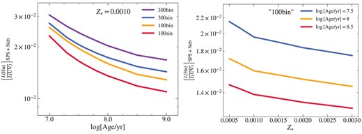
Variation of the H α-to-UV luminosity ratio derived from the SPS + Neb models with physical properties including stellar age, stellar metallicity, inclusion of binary stellar evolution, and upper-mass cutoff of the IMF. The SPS + Neb models are constructed using a constant SFH assumption.
The left panel of Fig. 6 indicates that the ratio predicted by the constant SFH models (|$\left[L(\rm{H\alpha })/L(\rm UV)\right]_{\rm \tt {SPS+Neb}}$|) at a fixed stellar metallicity is influenced by both the choice of upper-mass cutoff of the IMF and inclusion of binary stellar evolution. The H α luminosity increases by the presence of extremely massive stars with masses greater than 100 M⊙ and inclusion of energetic binary systems. For example, at |$\log [\rm {Age/yr}]=8.0$|, the |$L(\rm{H\alpha })/L(\rm UV)$| ratio grows by a factor of 1.2 and 1.3, respectively, from ‘100sin’ to the ‘100bin’ and ‘300bin’ models. The number of ionizing photons [and thus L(H α)] will decrease as massive O-stars evolve off the main sequence, whereas less massive stars will still contribute significantly to the non-ionizing UV luminosity. As a result, the |$L(\rm{H\alpha })/L(\rm UV)$| ratio decreases with increasing age as shown in the left panel of Fig. 6.
The right panel of Fig. 6 shows the sensitivity of |$\left[L(\rm{H\alpha })/L(\rm UV)\right]_{\rm \tt {SPS+Neb}}$| of ‘100bin’ model assumption to the stellar metallicity at various stellar population ages of the models. At a fixed stellar age, decreasing stellar metallicity increases the Hα-to-UV luminosity ratio. For example, |$\left[L(\rm{H\alpha })/L(\rm UV)\right]_{\rm \tt {SPS+Neb}}$| grows by a factor of ∼1.1 from Z* = 0.0020 to Z* = 0.0010 models, at |$\log [\rm Age/yr]=8.0$|. This relationship is expected given that lower metallicity stellar atmospheres (less opaque) result in higher effective temperatures and therefore harder ionizing spectra (Bicker, Fritze-v & Alvensleben 2005).
5 VARIATIONS OF THE AVERAGE PHYSICAL PROPERTIES OF GALAXIES WITH |$L(\rm{H\alpha })/L(\rm UV)$|
In addition to variations in the physical properties of galaxies such as stellar age and metallicity, variations in the strength of age-sensitive FUV spectral features with |$L(\rm{H\alpha })/L(\rm UV)$| may contain important information on burstiness. To investigate the above-mentioned variations, we divide the MOSDEF/LRIS sample into two |$L(\rm{H\alpha })/L(\rm UV)$| subsamples (hereafter referring to as low- and high-|$L(\rm{H\alpha })/L(\rm UV)$| bin) with an equal number of galaxies in each. When binning the galaxies, we are using the H α-to-UV luminosity ratio rather than the SFR[H α]-to-|$\rm SFR[\rm {UV}]$| ratio because the latter requires some assumptions of the SFH to convert luminosity to SFR, and when trying to probe the SFH (i.e. whether a galaxy has a bursty or constant SFH), it is useful to use a probe which is independent of such assumptions. The results of the measurements on the two subsamples are presented in the following sections.
5.1 Physical properties of galaxies versus |$L(\rm{H\alpha })/L(\rm UV)$|
The best-fitting SPS + Neb models to the rest-FUV composites are used to derive the average stellar age, metallicity, and continuum reddening of galaxies in each of the |$L(\rm{H\alpha })/L(\rm UV)$| bins (Table 2). In order for the SPS + Neb models to self-consistently explain all the observations, we checked that the |$L(\rm{H\alpha })/L(\rm UV)$| predicted by the best-fitting SPS + Neb model to each composite is in agreement with the mean ratio of all individual galaxies contributing to the composite as well as the average ratio directly measured from the rest-FUV and optical composite spectra.7
Average stellar population properties.
| Properties | Low|$\frac{L(\rm{H\alpha })}{L(\rm UV)}$| | High|$\frac{L(\rm{H\alpha })}{L(\rm UV)}$| |
|---|---|---|
| |$\left\langle L(\rm{H\alpha })/L({\rm {UV}})\right\rangle^{{a}} $| | 0.007 ± 0.002 | 0.035 ± 0.005 |
| |$\left\langle z \right\rangle$|b | 2.132 ± 0.031 | 2.185 ± 0.029 |
| |$\langle$|log [M*/M⊙]〉c | 9.88 ± 0.05 | 9.96 ± 0.06 |
| |$\left\langle R_{\rm e}\right\rangle (\rm {kpc})^{d}$| | 2.94 ± 0.23 | 2.33 ± 0.14 |
| |$\left\langle 12+\log (\rm O/H)\right\rangle ^{e}$| | 8.52 ± 0.02 | 8.39 ± 0.02 |
| |$\langle$|Z*/Z⊙〉f | 0.099 ± 0.010 | 0.085 ± 0.015 |
| |$\left\langle \log [\rm {Age/yr}]\right\rangle ^{g}$| | 8.4 ± 0.1 | 8.0 ± 0.2 |
| |$\langle$|E(B − V)cont〉h | 0.090 ± 0.010 | 0.074 ± 0.008 |
| |$\rm {\left\langle \text{SFR[SED]}\right\rangle }({\rm {M}}_{\odot }\, yr^{-1})^{\rm {i}}$| | 9.61 ± 2.73 | 10.64 ± 3.35 |
| |$\rm {\left\langle \text{SFR[H$\alpha $]}\right\rangle}({\rm M}_{\odot }\, yr^{-1})^{\rm j}$| | 8.57 ± 1.96 | 22.12 ± 2.04 |
| |$\rm {\left\langle \Sigma _{\text{SFR[H$\alpha $]}}\right\rangle}({\rm M}_{\odot }\, \rm yr^{-1} kpc^{-2})^{\rm k}$| | 0.16 ± 0.04 | 0.65 ± 0.10 |
| |$\langle$|E(B − V)neb〉l | 0.29 ± 0.03 | 0.49 ± 0.06 |
| |$\langle$|Wλ(Si iv)|$\rangle ({\mathring{\rm A}})^{\rm {m}}$| | 0.103 ± 0.018 | 0.146 ± 0.015 |
| |$\langle$|Wλ(C iv)|$\big \rangle \, ({\mathring{\rm A}})^{\rm n}$| | 0.206 ± 0.034 | 0.113 ± 0.024 |
| |$\langle$|Wλ(He ii)|$\big \rangle \, ({\mathring{\rm A}})^{\rm o}$| | 0.428 ± 0.032 | 0.684 ± 0.033 |
aMean dust-corrected H α-to-UV luminosity ratio.
bMean redshift.
cMean stellar mass.
dMean effective radius.
eMean gas-phase abundances
fStellar metallicity (Z⊙ = 0.0142 from Asplund et al. 2009).
gStellar population age.
hStellar continuum reddening.
iSED SFR measured from the FUV composite spectrum.
|$^{j}\, \rm{H\alpha }$| SFR measured from the optical composite spectrum.
|$^{k}\, \rm{H\alpha }$| SFR surface density.
lNebular reddening measured from the optical composite spectrum.
mEquivalent width of Si iv|$\, \lambda \lambda 1393,1403$|.
nEquivalent width of C iv|$\, \lambda \lambda 1548,1550$|.
0Equivalent width of He ii|$\, \lambda 1640$|.
Table 2 reports the average physical properties of galaxies in each |$L(\rm{H\alpha })/L(\rm UV)$| bin. The high-|$L(\rm{H\alpha })/L(\rm UV)$| subset exhibits, on average, an stellar population age of |$\log [\rm {Age/yr}]=8.0$|, compared to |$\log [\rm {Age/yr}]=8.4$| for the low-|$L(\rm{H\alpha })/L(\rm UV)$| galaxies, though the difference in age is significant at only the 2σ level. The stellar population age of the high-|$L(\rm{H\alpha })/L(\rm UV)$| galaxies is |$100\,$| Myr, longer than the dynamical time-scale of a few tens of Myr, implying that the high-|$L(\rm{H\alpha })/L(\rm UV)$| galaxies are not necessarily undergoing a burst of star formation. However, this conclusion comes with the caveat that the minimum SED-fitting age would be equivalent to the dynamical time-scale for a single initial burst of star formation. Using the SPS + Neb models, |$L(\rm{H\alpha })/L(\rm UV)$| increases by a factor of ∼1.1 from |$\log [\rm {Age/yr}] = 8.4$| to |$\log [\rm {Age/yr}] = 8.0$| for a fixed stellar metallicity (Fig. 6). The high-|$L(\rm{H\alpha })/L(\rm UV)$| subset exhibits an average |$L(\rm{H\alpha })/L(\rm UV)$| which is ∼5 times larger than that of the low-|$L(\rm{H\alpha })/L(\rm UV)$| subset. This implies that the difference in the average |$L(\rm{H\alpha })/L(\rm UV)$| ratio of the subsets cannot be solely attributed to the variation in the stellar age of those subsets. It is essential to examine other burst indicators, such as the strength of the FUV P-Cygni features in both bins, to find whether there is any strong evidence that the high-|$L(\rm{H\alpha })/L(\rm UV)$| subset traces recent starbursts. This is further discussed in the next section.
The effective radius (Re) of each galaxy is taken from van der Wel et al. (2014), and is defined as the radius that contains half of the total HST/F160W light. The SFR surface density (ΣSFR[H α]) of individual galaxies is then computed as
For an ensemble of galaxies, ⟨SFR[H α]〉 is computed by multiplying the dust-corrected ⟨L(H α)〉 measured from the optical composite spectrum by the conversion factor determined from the best-fitting SPS + Neb model. ⟨ΣSFR[H α]〉 is then computed using ⟨SFR[H α]〉 and mean Re of individual galaxies in each ensemble. ⟨SFR[H α]〉 and ⟨ΣSFR[H α]〉 increase significantly with increasing |$\left\langle L(\rm{H\alpha })/L(\rm {UV})\right\rangle $| between the two subsamples. While the instantaneous SFR (i.e. SFR[H α]) differs significantly between the two subsamples, SFR[SED] does not change significantly within the measurement uncertainties. By design, galaxies with higher |$L(\rm{H\alpha })/L(\rm {UV})$| have, on average, higher H α luminosities. However, this does not necessarily imply that these galaxies have higher H α-based SFRs than UV-based SFRs. The conversion factor that relates the dust-corrected L(H α) with SFR8 depends on stellar age, metallicity, and the hardness of the ionizing spectrum. As we show below, there is evidence that galaxies with higher |$L(\rm{H\alpha })/L(\rm {UV})$| have a harder ionizing spectrum than those with lower |$L(\rm{H\alpha })/L(\rm {UV})$| and, as such, they are likely to have a higher H α flux per unit SFR (see discussion in Section 5.2.2 and Section 6). The difference between the nebular and stellar reddening in the high-|$L(\rm{H\alpha })/L(\rm {UV})$| bin is ≃ 2.1 times larger when compared to the low-|$L(\rm{H\alpha })/L(\rm {UV})$|. The higher nebular reddening measured for the high-|$L(\rm{H\alpha })/L(\rm UV)$| bin is not surprising given that galaxies with larger L(H α) (i.e. higher SFRs) tend to be dustier (Förster Schreiber et al. 2009; Reddy et al. 2010; Kashino et al. 2013; Reddy et al. 2015, 2020).
5.2 Photospheric and stellar wind FUV spectral features versus |$L(\rm{H\alpha })/L(\rm UV)$|
Some FUV spectral features are strongly correlated with starburst age, metallicity, and IMF properties, making them excellent proxies for constraining the physical properties of the massive star population (Lamers et al. 1999; Pettini et al. 2000; Leitherer et al. 2001; Mehlert et al. 2002; Smith, Norris & Crowther 2002; Shapley et al. 2003; Keel, Holberg & Treuthardt 2004; Rix et al. 2004; Steidel et al. 2004; Leitherer et al. 2010; Cassata et al. 2013; Gräfener & Vink 2015; Chisholm et al. 2019; Reddy et al. 2022).
In continuous star formation, stars form at a relatively constant rate over time. As a result, the galaxy maintains a steady population of young, massive stars. This leads to a relatively stable presence of FUV P-Cygni features. In contrast, bursty star formation involves periods of intense star formation activity followed by periods of relative quiescence. During a starburst episode, the galaxy produces a large number of massive stars in a short period, which can lead to stronger FUV P-Cygni features as a result of the increased population of massive stars. And, during a post-burst episode, the equivalent widths of the features are expected to weaken (Walborn, Nichols-Bohlin & Panek 1985; Pellerin et al. 2002; Leitherer 2005; Vidal-García et al. 2017; Calabrò et al. 2021). The FUV spectral features discussed in this work are the P-Cygni component of Si iv|$\, \lambda \lambda 1393,1402$|, C iv|$\, \lambda \lambda 1548,1550$|, and the stellar component of He ii λ1640. The presence of C iv and Si iv P-Cygni features in a galaxy’s spectrum suggests the existence of massive stars with M* ≥ 30 M⊙ and short main-sequence lifetime of |$\sim 2{-}5\,$| Myr, and therefore is an indicator of the early stages of star formation (Leitherer & Heckman 1995; Pettini et al. 2000; Leitherer et al. 2001; Shapley et al. 2003; Quider et al. 2009). The origin of the broad He ii λ1640 stellar wind emission observed in the spectra of local galaxies is the massive short-lived and extremely hot Wolf–Rayet stars (Schaerer 1996; de Mello et al. 1998; Crowther 2007; Shirazi & Brinchmann 2012; Cassata et al. 2013; Visbal, Haiman & Bryan 2015; Crowther et al. 2016; Nanayakkara et al. 2019). The fraction of WR stars declines with decreasing stellar metallicity. Therefore, another mechanism is needed to explain the observation of He ii λ1640 at high-redshift galaxies where the metallicity is lower compared to local galaxies. One possible explanation for such observation is the abundance of binary systems at high redshifts that can result in an increase in the fraction of WR stars in low-metallicity environments (Shapley et al. 2003; Cantiello et al. 2007; de Mink et al. 2013). In fact, according to previous studies, when single evolution SPS models are compared to the models including binary evolution in low stellar metallicity, the He ii stellar feature is best reproduced by the latter (Shirazi & Brinchmann 2012; Gutkin, Charlot & Bruzual 2016; Stanway, Eldridge & Becker 2016; Steidel et al. 2016; Eldridge et al. 2017; Senchyna et al. 2017; Smith, Götberg & de Mink 2018; Chisholm et al. 2019; Saxena et al. 2020; Reddy et al. 2022). Therefore, fitting the observed rest-FUV composite spectra with the SPS models that include binary stellar evolution is necessary in order to study the variations in the strength of stellar He ii λ1640 emission.
5.2.1 SPS + Neb Model Predictions of FUV Spectral Features
Based on the SPS + Neb models, we show an example of the sensitivity of Si iv, C iv, and He ii stellar features to the stellar age, metallicity, and Mcutoff of the IMF in Fig. 7. The equivalent widths (Wλ) of these features are also shown in the inset panels. These equivalent widths are measured by directly integrating across each line (above the line of unity) in the continuum-normalized models. In each panel, we only adjust one physical parameter at a time and keep the other two unchanged. The fixed values are chosen based on the average parameters derived from the composite spectra of all galaxies in the MOSDEF/LRIS sample.
![Variation of the continuum-normalized SPS + Neb models with stellar metallicity (top panel), stellar age (middle panel), and upper-mass cutoff of the IMF (bottom panel). In each panel, only the specified parameter in the lower left is relaxed to change, while the parameters indicated in the upper left are held fixed. In all panels, the ionization parameter and nebular metallicity are held fixed to the average values of the MOSDEF-LRIS sample (log U = −3.0, log [Zneb/Z⊙] = −0.4; from Reddy et al. 2022). Each of the three columns presented in this figure corresponds to a particular feature: Si iv P-Cygni, C iv P-Cygni, and He ii stellar winds. The inset panels indicate the equivalent width of each line in each model. The shaded pink indicates the regions by which the width measurements are performed for each feature.](https://oup.silverchair-cdn.com/oup/backfile/Content_public/Journal/mnras/526/1/10.1093_mnras_stad2842/1/m_stad2842fig7.jpeg?Expires=1749175347&Signature=3mJaQfhYv-gT5vZopai4sJLlW4fCXHQ~xAVdtALA44b9ckbCVyJ007Toica3TkCPEMR3GclAOAChOKEG1fvnuZu0oQO-UtHwA42q8VzXTKRpNN0OKv5lsB9nl~D5905I4O~i~ahGRhkmHRUBSxH4kJ48wwJmrZiO3pLLCSoB9Qmfl3Vgf62P6H3Lo6M4djinPrtjnTf1NpC~1uhJ5qRDrut63nJs~-6ydc-zom8Mat54ds9o4hHo4axRJK37aqhqMK9dcX-s2tj-EViiGHru-Mw3xKV5I3W7Np4i02fDmwG~jy4jkn5mAU99W-tuKqqZbB~E6Wo0q3nZf4KuqLLe7w__&Key-Pair-Id=APKAIE5G5CRDK6RD3PGA)
Variation of the continuum-normalized SPS + Neb models with stellar metallicity (top panel), stellar age (middle panel), and upper-mass cutoff of the IMF (bottom panel). In each panel, only the specified parameter in the lower left is relaxed to change, while the parameters indicated in the upper left are held fixed. In all panels, the ionization parameter and nebular metallicity are held fixed to the average values of the MOSDEF-LRIS sample (log U = −3.0, log [Zneb/Z⊙] = −0.4; from Reddy et al. 2022). Each of the three columns presented in this figure corresponds to a particular feature: Si iv P-Cygni, C iv P-Cygni, and He ii stellar winds. The inset panels indicate the equivalent width of each line in each model. The shaded pink indicates the regions by which the width measurements are performed for each feature.
The top panel of Fig. 7 compares three constant SFH models with fixed stellar population age of |$\log [\rm Age/yr]=8.0$|, fixed upper-mass cutoff of |$M_{\rm cutoff}=100\, {\rm M}_{\odot }$|, and varying metallicities of Z* = {0.0010, 0.0020, 0.0030}. As depicted by the inset panels, as the metallicity increases from Z* = 0.0010 to Z* = 0.0030, the equivalent widths of C iv and Si iv P-Cygni emission become ∼2.3 and ∼2.5 times larger, respectively. This is due to the fact that these P-Cygni features are sensitive to mass-loss rate, which increases as metallicity increases. In the case of He ii, the model with lowest metallicity (Z* = 0.0010) exhibits the largest equivalent width compare to the higher metallicity models. This is due to the fact that stars with lower metallicity at given ages have harder ionizing spectra.
The middle panel of Fig. 7 shows three models with fixed metallicity of Z* = 0.0014, fixed mass cutoff of |$M_{\rm cutoff}=100\, {\rm M}_{\odot }$|, and varying stellar ages of |$\log [\rm Age/yr]=\lbrace 7.0,7.5,8.0\rbrace$|. The inset panels demonstrate that the younger stellar population model (|$\log [\rm Age/yr]=7.0$|) show a larger equivalent width of Si iv, C iv, and He ii by a factor of ∼2.1, ∼1.6, and ∼1.5, respectively, when compared to the model with a higher age (|$\log [\rm Age/yr]=8.0$|). This prediction again demonstrates that the photospheric and stellar wind spectral features are strong at the early stages of star formation
The bottom panel of Fig. 7 depicts two SPS + Neb models with fixed stellar age of |$\log [\rm Age/yr]=8.0$| and stellar metallicity of Z* = 0.0014 and varying upper-mass cutoff of Mcutoff/M⊙ = {100, 300}. The inset panels indicate that changing the mass cutoff of the IMF from 100 to |$300\, {\rm M}_{\odot }$| causes the equivalent widths of Si iv, C iv, and He ii to grow ∼1.1, ∼1.1, and ∼1.2 times larger.
5.2.2 Observed FUV spectral featurbees in bins of |$L(\rm{H\alpha })/L(\rm UV)$|
As shown in Section 5.2.1, the model-predicted equivalent widths of Si iv, C iv, and He ii are sensitive to stellar age, metallicity, and less sensitive to the high-mass cutoff of the IMF. In this section, we examine the variations in the observed equivalent widths of those FUV spectral features from the composite spectra of the two |$L(\rm{H\alpha })/L(\rm UV)$| subsamples. The advantage of analysing equivalent widths of the observed features is that they are unaffected by dust or aperture uncertainties. In addition, the observed equivalent widths are insensitive to the model assumptions (e.g. constant versus instantaneous burst SFH).
The average rest-frame equivalent widths (|$\langle$|Wλ〉) for each of the above-mentioned FUV spectral features are measured by directly integrating across each line in each of the continuum-normalized composite spectra shown in Fig. 8 and are reported in Table 2. To ensure unbiased measurements, we utilize identical wavelength intervals for each bin. These wavelength intervals are derived based on the regions that the lines occupy in the SPS + Neb models. These regions are highlighted in Fig. 7. The errors in Wλ are measured by perturbing the continuum-normalized spectra according to the error in spectra and repeating the measurements many times. The uncertainty is determined by the standard deviation of these perturbations. The final reported uncertainties include the error associated with the normalization process.
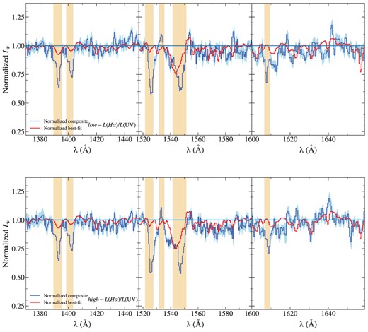
Continuum-normalized composite spectra (blue) of the two |$L(\rm{H\alpha })/L(\rm UV)$| subsamples from which the equivalent width measurements are performed. The physical properties of each of the bins, as well as, Wλ(Si iv), Wλ(C iv), and Wλ(He ii) measurements are listed in Table 2. Those regions that are not included in the fitting process are shaded in orange.
Fig. 9 shows the comparison between the average rest-frame equivalent widths of Si iv, C iv, and He ii in the |$L(\rm{H\alpha })/L(\rm UV)$| subsamples. No significant differences are found in |$\left\langle W_{\lambda }(\rm {Si\, {\small IV}})\right\rangle $|, and |$\left\langle W_{\lambda }(\rm {C\, {\small IV}})\right\rangle $| between the low- and high-|$L(\rm{H\alpha })/L(\rm UV)$| bins within the measurement uncertainties. However, |$\left\langle W_{\lambda }(\rm {He\, {\small II}})\right\rangle $| grows by a factor of ∼1.7 from the low- to high-|$L(\rm{H\alpha })/L(\rm UV)$| bin. If galaxies with higher |$L(\rm{H\alpha })/L(\rm UV)$| are undergoing a burst of star formation, then we would expect them to have higher C iv and Si iv P-Cygni emission equivalent widths relative to galaxies with lower |$L(\rm{H\alpha })/L(\rm UV)$|.
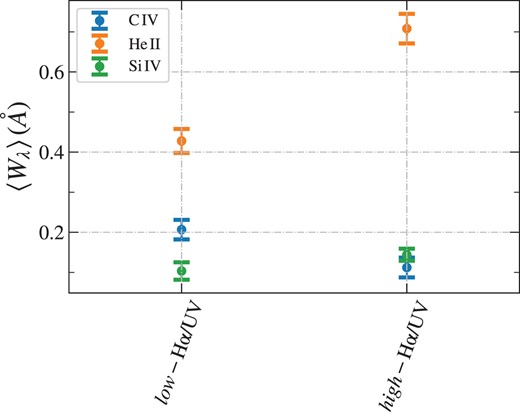
Comparison of the average equivalent widths of Si iv|$\, \lambda \lambda 1393,1402$|, C iv|$\, \lambda \lambda 1548,1550$|, and He ii λ1640 stellar emission lines measured from the continuum-normalized spectra of the two bins reported in Table 2.
While Si iv and C iv P-Cygni emissions are prominently stellar in origin, this is not the case for He ii. The extremely hot sources that produce stellar He ii emission also generate enough |$\rm {He^{+}}\,$| ionizing photons with wavelengths of |$\lambda \langle 228\, {\mathring{\rm A}}$| to yield nebular He ii emission due to recombination, which complicates the interpretation of the He ii emission. Based on the previous studies (e.g. Steidel et al. 2016; Reddy et al. 2022), we adopt the following procedure to disentangle the stellar and nebular components. We measure the observed nebular He ii intensity by subtracting the best-fitting SPS + Neb model from the composite spectrum of each bin using the ‘100bin’ and ‘300bin’9 model assumptions. Because the best-fitting model identifies the stellar component, the subtraction of the best-fitting model from the observed spectrum is assumed to be purely nebular. The observed nebular He ii intensity is then dust-corrected assuming |$\langle$|E(B − V)neb 〉 and the Cardelli et al. (1989) extinction curve, where |$\langle$|E(B − V)neb 〉 is measured directly from the optical composite spectrum. The model-predicted nebular He ii intensity is derived by using the best-fitting SPS model of each bin as an input to the Cloudy photoionization code. The comparison between the model-predicted and observed nebular He ii emission in terms of relative intensity, |$\left\langle \rm{He\,{\small II}}/\rm{H\beta }\right\rangle $|, is shown in Fig. 10 for the |$L(\rm{H\alpha })/L(\rm UV)$| subsamples. The model-predicted and observed nebular He ii intensities measured for the low-|$L(\rm{H\alpha })/L(\rm UV)$| bin agree within the 3σ uncertainty for both of the mass cutoff assumptions. However, the model prediction of the nebular He ii intensity does not fully account for the observed nebular He ii intensity in the high-|$L(\rm{H\alpha })/L(\rm UV)$| bin even with an increase in the upper-mass cutoff of the IMF.
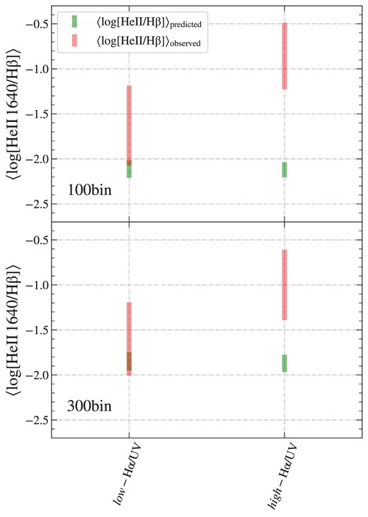
Comparison of the model-predicted nebular He ii λ1640 relative intensity, |$\left\langle \rm{He\,{\small II}}/\rm{H\beta }\right\rangle $|, derived from the Cloudy code and the observed dust-corrected relative intensity measured by subtraction of the best-fitting SPS + Neb model from the composite spectrum for each |$L(\rm{H\alpha })/L(\rm UV)$| subsample and different model assumptions. The coloured bars show the ±3σ range of the measurement uncertainties.
Our results indicate that recent SF activity, and low metallicity cannot explain the difference in the He ii emission of galaxies in the two |$L(\rm{H\alpha })/L(\rm UV)$| bins because the stellar age and metallicity derived for the two bins are similar within their respective uncertainties. Next, we investigate whether a top heavy IMF can account for such a difference. First, we separate the nebular and stellar components of the He ii emission. We then compare the observed nebular He ii intensity to that predicted by the Cloudy photoionization model using various assumptions on the upper-mass limit of the IMF. We find that even a top heavy IMF model (Mcutoff = 300M⊙) is unable to accurately predict the observed nebular He ii intensity of the high-|$L(\rm{H\alpha })/L(\rm UV)$| bin. Another potential contributor that gives rise to the He + ionizing photons budget in low-metallicity star-forming galaxies is discussed below.
Schaerer, Fragos & Izotov (2019) suggested that high-mass X-ray binaries (HMXBs) are a primary source for producing He + ionizing photons in low-metallicity star-forming galaxies. They found that only SPS models that include HMXBs are able to reproduce the observed relative intensity of nebular He ii emission (|$\rm{He\,{\small II}}/\rm{H\beta }$|). Studies of both the local and high-redshift universe have suggested that the X-ray luminosity (LX) of HMXBs in star-forming galaxies increases with SFR (Bauer et al. 2002; Nandra et al. 2002; Seibert, Heckman & Meurer 2002; Grimm, Gilfanov & Sunyaev 2003; Gilfanov, Grimm & Sunyaev 2004; Persic et al. 2004; Reddy & Steidel 2004; Persic & Rephaeli 2007; Lehmer et al. 2008, 2010), which is expected owing to the young ages of HXMBs (|$\sim 10\,$| Myr). Several studies have indicated that LX per unit SFR in star-forming galaxies elevates at high redshift (e.g. Basu-Zych et al. 2013a; Lehmer et al. 2016; Aird, Coil & Georgakakis 2017). This enhancement in LX/SFR with redshift may be due to the lower metallicities of high-redshift galaxies, which results in more luminous (and possibly more numerous) HMXBs (Douna et al. 2015; Brorby et al. 2016). In fact, observational studies have shown evidence of several ultraluminous X-ray sources in nearby galaxies with low metallicities (e.g. Mineo, Gilfanov & Sunyaev 2012; Prestwich et al. 2013; Basu-Zych et al. 2013b). Following the idea that LX/SFR is metallicity dependent, Brorby et al. (2016) parameterized the LX–SFR–Z relationship, where Z is the gas-phase metallicity, for a sample of local star-forming galaxies as
Fornasini et al. (2019) studied a sample of MOSDEF galaxies with available X-ray data to investigate the LX/SFR and Z relationship at redshift z ∼ 2. They found that for both H α- and SED-based SFRs, the LX–SFR–Z relation is in good agreement with that of the Brorby et al. (2016) relation for local galaxies (equation 5). The results obtained were not affected by the assumed L(H α) to SFR[H α] conversion factor. We incorporate SFR[H α] and SFR[SED] into equation (5) to calculate the average X-ray luminosities for the |$L(\rm{H\alpha })/L(\rm UV)$| subsets. We find that the average X-ray luminosity of the high-|$L(\rm{H\alpha })/L(\rm UV)$| subset is three times greater with SFR[H α], and 1.4 times greater with SFR[SED] when compared to the average X-ray luminosity of the low-|$L(\rm{H\alpha })/L(\rm UV)$| subset. The statistical differences between the average X-ray luminosities derived using SFR[H α] and SFR[SED] are at 5σ and 2σ levels, respectively. The increase in <LX 〉 with increasing |$L(\rm{H\alpha })/L(\rm UV)$| may indicate the presence of luminous HMXBs, which in turn could explain the high nebular He ii emission observed for galaxies with high |$L(\rm{H\alpha })/L(\rm UV)$| ratios. Considering that an increase in <LX 〉 is also observed when using SFR[SED], the conclusion about the existence of HMXBs may be reliably drawn. However, this conclusion is only robust at a 2σ statistical significance level owing to the large uncertainties of the average SED-based SFRs.
6 SUMMARY AND CONCLUSION
We examine the effectiveness of the dust-corrected globally measured H α-to-UV luminosity ratio in tracing burstiness for typical star-forming galaxies at z ∼ 2. We use the MOSDEF survey to explore stellar population properties differences in bins of |$L(\rm{H\alpha })/L(\rm {UV})$|.
In the first part of this analysis, we employ the HST imaging of 310 star-forming galaxies (MOSDEF/MORPH sample) drawn from the MOSDEF survey to construct the SFR surface density and stellar age maps. We use a Voronoi binning technique to group the pixels based on their S/N. We then study the distribution of ΣSFR[SED] and stellar age of Voronoi bins within each galaxy using a morphological metric called patchiness (P). Patchiness is sensitive to deviations from average, therefore galaxies that are undergoing a burst of star formation contain regions with higher ΣSFR[SED] and younger stellar age than the mean value for the entire galaxy and are expected to exhibit higher P(ΣSFR[SED]) and/or |$P(\rm Age)$|. We find no correlation between |$L(\rm{H\alpha })/L(\rm UV)$| and P(ΣSFR[SED]), as well as between |$L(\rm{H\alpha })/L(\rm UV)$| and |$P(\rm Age)$|. We suggest that the globally averaged |$L(\rm{H\alpha })/L(\rm UV)$| does not trace stochastic SFH over a time-scale of |$\sim 10\,$| Myr, which is the typical dynamical time-scale probed by the Voronoi bins. We suggest that this lack of correlation may be because of the uncertainties related to the variations in the stellar dust attenuation curve, limited dynamical time-scale and spatial resolution probed by the Voronoi bins.
In the second part of this analysis, we use a rest-FUV spectroscopic sample obtained by LRIS (MOSDEF/LRIS sample) to study the average physical properties of z ∼ 2 star-forming galaxies in bins of |$L(\rm{H\alpha })/L(\rm UV)$|. We use the BPASS constant SFH models combined with the nebular continuum emission generated by the Cloudy radiative transfer code (SPS + Neb models) as our theoretical basis to address the effect of different physical assumptions on the model-predicted |$L(\rm{H\alpha })/L(\rm UV)$|. As suggested by other studies, the H α-to-UV ratio predicted by SPS + Neb models increases for younger stellar populations, or when the upper end of the IMF increases. The inclusion of binary stellar evolution or lowering the stellar metallicity of the models also cause a rise in the predicted ratio. We divide the 124 galaxies in the MOSDEF/LRIS sample into two bins of |$L(\rm{H\alpha })/L(\rm UV)$| with an equal number of galaxies in each to investigate whether the variation observed in the dust-corrected H α-to-UV ratio is related to differences in stellar age, metallicity, and/or upper-end mass of the IMF as suggested by the SPS theoretical models. The main conclusions of the second part of the paper are as follows:
The average stellar population age estimated for the high-|$L(\rm{H\alpha })/L(\rm UV)$| bin is |$\log [\rm {Age/yr}]=8.0\pm 0.2$|, compared to |$\log [\rm {Age/yr}]=8.4\pm 0.1$| for the low-|$L(\rm{H\alpha })/L(\rm UV)$| bin. We find no significant variation in the stellar metallicity between the low- and high-|$L(\rm{H\alpha })/L(\rm UV)$| bin within the measurement uncertainties. The stellar population age of |$100\,$| Myr derived for the high-|$L(\rm{H\alpha })/L(\rm UV)$| bin is longer than the dynamical time-scale of a few tens of Myr, implying that the high-|$L(\rm{H\alpha })/L(\rm UV)$| galaxies are not necessarily undergoing a burst of star formation.
Galaxies with higher |$L(\rm{H\alpha })/L(\rm UV)$| have on average higher H α luminosities. Such galaxies also have strong He ii λ1640 emission, but do not exhibit significantly different EWs of Si iv|$\, \lambda \lambda 1393,1402$|, C iv|$\, \lambda \lambda 1548,1550$| P-Cygni emissions. These results suggest that the higher Ha/UV ratio of these galaxies is due to their harder ionizing spectra, rather than a higher SFR[H α] relative to SFR[UV]. The lack of variations in the strength of the P-Cygni emissions between the two |$L(\rm{H\alpha })/L(\rm UV)$| subsamples is expected given the insignificant differences found between the stellar age and metallicity of the two subsamples.
The difference between the strength of the observed He ii emission of the low- and high-|$L(\rm{H\alpha })/L(\rm UV)$| subsamples can be further investigated when the nebular and stellar components of the He ii line are disentangled. We find that the model-predicted nebular He ii intensity cannot accurately predict the observed amount for the high-|$L(\rm{H\alpha })/L(\rm UV)$| bin even if the upper-mass limit of the IMF is increased from |$M_{\rm cutoff}=100$| to |$300\, {\rm M}_{\odot }$|. According to recent studies, low metallicity star-forming galaxies get the majority of their He + ionizing photons from HMXBs (Schaerer et al. 2019). We measure the X-ray luminosity of each bin using the LX–SFR–Z relation found by Brorby et al. (2016) for local galaxies. Fornasini et al. (2019) found that the LX–SFR–Z relation for z ∼ 2 galaxies is in good agreement with the Brorby et al. (2016) local relation for both H α- and SED-based SFRs. We find that the X-ray luminosity is on average larger for galaxies with higher |$L(\rm{H\alpha })/L(\rm UV)$| regardless of the assumed SFR indicator. This result may suggest the presence of luminous HMXBs, which could explain the high nebular He ii emission observed for galaxies with high H α-to-UV ratios. As HMXBs have short lifespans (a few Myr), they effectively indicate recent star formation. Nonetheless, the potential abundance of HMXBs in the high-|$L(\rm{H\alpha })/L(\rm UV)$| group does not directly imply that galaxies in this subset primarily experience a bursty SFH, since massive stars and HMXBs are being continuously formed even in a constant SFH. In addition, the idea that the high-|$L(\rm{H\alpha })/L(\rm UV)$| sample is in a burst mode of star formation is not supported by the fact that the equivalent width of the C iv and Si iv P-Cygni features do not vary between the two subsamples. The presence of a more intense ionizing spectrum in galaxies with higher |$L(\rm{H\alpha })/L(\rm UV)$| ratios can be backed by the abundance of HMXBs in these galaxies.
Our results cast doubt upon the reliability of H α-to-UV luminosity ratio in tracing bursty SFH of typical star-forming galaxies at z ∼ 2. This is due to the absence of evidence suggesting that galaxies with higher |$L(\rm{H\alpha })/L(\rm UV)$| are experiencing a burst, based on their average stellar population age and the lack of variation in P-Cygni features compared to galaxies with lower |$L(\rm{H\alpha })/L(\rm UV)$|. There is one important implication of this work. It is proposed that star-forming galaxies may be in a bursty phase of star formation at the beginning of the reionization epoch, producing enough ionizing photons to reionize the intergalactic medium. If such is the case, it is important to validate the tracer of burstiness which is commonly used in the literature, and whether there are other phenomena that can affect the H α-to-UV ratio. Using the next-generation telescopes, we will have access to even more high-quality data to study the H α-to-UV ratio variations in more detail. For example, JWST can provide high-resolution rest-FUV spectra of high redshift galaxies to aid in constraining the mode of SFH and/or hardness of the ionizing spectrum and the causes of the variations in the H α-to-UV ratio.
Several studies of high redshift galaxies have found evidence of bursty SFHs by comparing H α and UV SFRs (e.g. Atek et al. 2022 at z ∼ 1.1, and Faisst et al. 2019 at z ∼ 4.5). These works suggest that the excess found in the H α SFR relative to the UV SFR can only be explained by additional bursts of star formation on top of an underlying smooth star formation. The aforementioned studies have found that SFR[H α]/SFR[UV] ratio is preferentially higher for lower mass galaxies. Galaxies of lower masses, which are also likely to have a lower metallicity, may be conducive to an IMF that is top-heavy (Tremonti et al. 2004; Dalcanton 2007; Lara-López et al. 2010; Peeples & Shankar 2011; Andrews & Martini 2013; Lilly et al. 2013; Zahid et al. 2014; Chisholm, Tremonti & Leitherer 2018), and therefore one must be very careful in interpreting the H α-to-UV ratio for such galaxies. The equivalent width of the stellar photosphere features investigated in this work (Section 5.2) is less affected by the uncertainties associated with the |$L(\rm{H\alpha })/L(\rm UV)$| ratio, such as variations in ionizing escape fraction, stochastic IMF, and dust reddening. Hence, the equivalent width of FUV stellar features (e.g. c iv, and Si iv) may more reliably trace recent bursts of star formation than the H α-to-UV ratio. None the less, it is suggested that future studies use higher S/N rest-frame FUV spectra and increased sample sizes to more effectively compare the effectiveness of P-Cygni features in tracing star formation burstiness against the H α-to-UV ratio.
ACKNOWLEDGEMENTS
This work is based on observations taken by the 3D-HST Treasury Program (GO 12177 and 12328) with the NASA/ESA HST, which is operated by the Association of Universities for Research in Astronomy, Inc., under NASA contract NAS5-26555. In addition, we would like to acknowledge that this work made use of v2.2.1 of the Binary Population and Spectral Synthesis (BPASS) models as described in Eldridge et al. (2017), and Stanway & Eldridge (2018). The MOSDEF team acknowledges support from an NSF AAG collaborative grant (AST-1312780, 1312547, 1312764, and 1313171), grant AR-13907 from the Space Telescope Science Institute, grant NNX16AF54G from the NASA ADAP program, and Chandra archival award AR6-17011X. This work would not have been possible without the generous contributions from the 3D-HST collaboration. The MOSDEF data were obtained at the WM Keck Observatory, which is operated as a scientific partnership among the California Institute of Technology, the University of California and the National Aeronautics and Space Administration. The Observatory was made possible by the generous financial support of the WM Keck Foundation. We recognize and acknowledge the very significant cultural role and reverence that the summit of Mauna Kea has always had within the indigenous Hawaiian community. We are most fortunate to have the opportunity to conduct observations from this mountain.
7 DATA AVAILABILITY
In this work, we use spectroscopic redshifts and rest-frame optical line measurements obtained from the MOSFIRE Deep Evolution Field (MOSDEF) survey (Kriek et al. 2015). This is publicly available at https://mosdef.astro.berkeley.edu/.
We also use photometry obtained from the CANDELS (Grogin et al. 2011; Koekemoer et al. 2011) and reprocessed by the 3D-HST grism survey team (Brammer et al. 2012; Skelton et al. 2014; Momcheva et al. 2016). The data sets and catalogues can be found at https://archive.stsci.edu/prepds/3d-hst/.
We analyze the Far-UV spectra obtained by the Low Resolution Imagerand Spectrometer (LRIS; Oke et al. 1995; Steidel et al. 2004). Topping et al. (2020) and Reddy et al. (2022) contain information about the MOSDEF/LRIS data reduction. MOSDEF/LRIS data sets are available upon request.
Footnotes
According to Reddy et al. (2012), if the stellar ages are constrained to be older than the typical dynamical time-scale, SED models with either constant or exponentially rising SFHs are best at reproducing the SFR of galaxies at z ∼ 2. The study also found that assuming exponentially rising SFHs leads to stellar population age estimates that are on average 30 per cent older than those obtained under the assumption of constant SFHs. Our sample of galaxies, assuming both exponentially rising and declining SFHs, exhibit SFRs that are typically within 0.03 dex of those obtained under constant SFHs, which is within the usual measurement uncertainties of SED-derived SFRs.
The SED parameters, such as SFR, stellar age, etc., are determined for individual Voronoi bins by performing SED fitting on resolved scales, as explained in Section 2.4. However, determining the uncertainty or noise in each SED parameter is a time-consuming process due to the large number of Voronoi bins and galaxies involved (Fetherolf et al. 2023). To address this challenge, we chose 50 galaxies with stellar population parameters similar to the overall sample and perturbed the resolved photometric fluxes based on their respective errors. We conducted SED fitting on these perturbed values, and the standard deviation of the SED parameters from the models with the lowest χ² were treated as the 1σ uncertainty in the SED parameters.
The same procedure outlined in Section 4.1 is applied to construct the optical composite spectrum (e.g. Shivaei et al. 2018; Reddy et al. 2020; Rezaee et al. 2021). The Python code presented in https://github.com/IreneShivaei/specline/ is used in constructing the optical composite spectra here.
The conversion factors between the dust-corrected H α luminosity into SFR[H α] are 2.675, 4.888, 2.102, and |$4.236\times 10^{-42},{\rm M}_{\odot }\rm {yr^{-1}erg^{-1}s}$| for the ‘|$0.07\, Z_{\odot },$|100sin’, ‘|$1.41\, Z_{\odot },$|100sin’, ‘|$0.07\, Z_{\odot },$|100bin’, and ‘|$1.41\, Z_{\odot },$|100bin’ models, respectively. This is based on the Chabrier (2003) IMF.
When fitting the FUV composite spectra with the ‘300bin’ SPS + Neb models, they can still reproduce all the FUV features discussed in this work. The best-fitting stellar population age, metallicity, and continuum reddening of the high-|$L(\rm{H\alpha })/L(\rm UV)$| subsample obtained with the ‘300bin’ model are |$\left\langle \log [\rm Age/yr]\right\rangle =8.0\pm 0.2$|, <Z* 〉 = 0.084 ± 0.011, and <E(B − V)cont 〉 =0.067 ± 0.005.
References
Author notes
Nasa Hubble Fellow.
NASA Postdoctoral Program Fellow.
