


ABSTRACT
De-excitation gamma-ray lines, produced by nuclei colliding with protons, provide information about astrophysical environments where particles have kinetic energies of 10–100 MeV per nucleon. In general, such environments can be categorized into two types: the interaction between non-thermal MeV cosmic rays and ambient gas, and the other is thermal plasma with a temperature above a few MeV. In this paper, we focus on the latter type and investigate the production of de-excitation gamma-ray lines in very hot thermal plasma, especially the dependence of the line profile on the plasma temperature. We have calculated the line profile of prompt gamma rays from 12C and 16O and found that when nuclei have a higher temperature than protons, gamma-ray line profiles can have a complex shape unique to each nucleus species. This is caused by anisotropic gamma-ray emission in the nucleus rest frame. We propose that the spectroscopy of nuclear de-excitation gamma-ray lines may enable to probe energy distribution in very hot astrophysical plasmas. This diagnostics can be a new and powerful technique to investigate the physical state of a two-temperature accretion flows onto a black hole, especially the energy distributions of the protons and nuclei, which are difficult to access for any other diagnostics.
1 INTRODUCTION
Atomic nuclei colliding with protons can go into their excited states when the kinetic energy of protons is larger than a few MeV in the nucleus rest frame. Immediately after, the excited nuclei emit gamma rays with a specific energy. Such gamma rays, so-called nuclear de-excitation lines, can provide us with unique information about the conditions of production sites of protons and nuclei in the MeV range and their energy distributions and compositions. In astrophysics, understanding the production of such MeV particles is essential in broad topics, for instance, low-energy MeV cosmic rays and their total amount of energy (Ramaty, Kozlovsky & Lingenfelter 1979; Ramaty, Kozlovsky & Lingenfelter 1996), particle acceleration processes in supernova remnants and solar flares (Murphy et al. 2009; Nobukawa et al. 2018), and a very hot plasma formed by relativistic compact objects (Aharonian & Sunyaev 1984; Kafexhiu, Aharonian & Barkov 2019a, b). Generally, observations of nuclear de-excitation lines can be a direct probe for the following two environments: non-thermal MeV cosmic rays colliding with ambient cold gas and thermal plasma with a temperature above 1010 K (Aharonian 2004).
The diagnostics of low-energy cosmic rays using the de-excitation lines was noticed with the report of 3–7 MeV gamma-ray excess from the Orion complex observed with COMPTEL/CGRO (Bloemen et al. 1994, 1997). The excess in 3–7 MeV was interpreted as the combination of 4.44 MeV from 12C* and 6.13 MeV from 16O*. Furthermore, the reported line was broad, and its width was larger than that of collision between energetic protons in cosmic rays and nuclei in ambient gas (in this case, the line width is ∼100 keV). Alternatively, the authors interpreted that non-thermal nuclei in cosmic rays collide with protons in the ambient matter, and the de-excitation lines were Doppler-broadened. While the reported gamma-ray excess was found as a false detection after the background model and analysis method were revisited (Bloemen et al. 1999), it stimulated detailed modelling of the nuclear gamma-ray line due to collisions between non-thermal particles and cold gas (Ramaty, Kozlovsky & Lingenfelter 1995; Bykov, Bozhokin & Bloemen 1996; Ramaty et al. 1996; Bozhokin & Bykov 1997).
The detailed modelling showed that the line profile can have a complex shape under certain situations. Bykov et al. (1996) and Kozlovsky, Ramaty & Lingenfelter (1997) calculated the de-excitation gamma-ray line profiles assuming that nuclei which have kinetic energy larger than ∼10 MeV nucleon−1 collide with ambient protons, and they showed that the line profile could have several peaks. This is caused by the fact that the gamma-ray line emission in the nucleus rest frame is anisotropic, which results in subsequent Doppler broadening of the line shape. In this work, we refer to such a complex line-shape formation as line splitting. The line splitting can also occur when nuclei collide with collimated non-thermal protons, e.g. solar flares (Ramaty et al. 1979; Murphy, Kozlovsky & Ramaty 1988; Werntz, Lang & Kim 1990). These works revealed that the energy distributions of accelerated protons and nuclei in the MeV range affect the profile of de-excitation lines, and we can derive their energy distributions by the line profile modelling, including the line splitting effect.
While the line profile of de-excitation gamma rays is studied well in the above non-thermal cases, its property under thermal environments still needs to be studied in the same manner. Since the de-excitation gamma rays can also be produced in thermal plasma with a temperature above 1010 K, e.g. hot plasma surrounding relativistic compact objects and in supernova remnants, understanding the line profile under such thermal environments can provide a unique way to study the two-temperature plasma where electrons and ions have different temperatures and pre-acceleration of low-energy cosmic rays, which cannot be accessible with other tools. Thus, in this work, we aim to examine the basic properties of the line profile of nuclear de-excitation gamma rays under the thermal environments, particularly its dependence on emissivity and proton and nucleus temperatures, and conditions in which the line splitting occurs.
Here, we mainly focus on the 4.44 MeV and 6.13 MeV gamma-ray lines from 12C (p, pγ) 12C and 16O (p, pγ) 16O. First, we explain the physics of line splitting in Section 2 and then describe the method we used to calculate the line profile in Section 3. Section 4 describes the cross-section data used for the angular distribution of the nuclear gamma rays in the nucleus rest frame. In Section 5, we show the gamma-ray line profile in the thermal environments and describe its basic features without assuming any specific astrophysical situations. In Section 6, we discuss possible astrophysical applications, such as a unique probe to the two-temperature plasma in accreting flows on black holes. Finally, we summarize our work in Section 7.
2 LINE SPLITTING IN THE PROFILE OF PROMPT GAMMA-RAY LINE
When a nucleus interacts with a proton with enough kinetic energy, the nucleus may be excited into a higher nucleus state. Then, a prompt gamma ray is emitted immediately, with a time-scale from fs to ms. The distribution of gamma-ray emission follows multipole radiation corresponding to the spin state of the excited state. Note that here the quantization axis in the nucleus rest frame is determined by the incoming proton direction. In practice, the angular distribution of emitted gamma rays is usually described well with the superposition of several multipole expansion terms because there are several spin states in the excited states (Kolata, Auble & Galonsky 1967; Ramaty et al. 1979). The angular distribution has been measured for several species experimentally, and it depends on the nuclear species and the projectile energy, that is, here, the kinetic energy of protons (Lang et al. 1987; Lesko et al. 1988).
Suppose a nucleus has a kinetic energy larger than an excited state, so that it could change the states when interacting with a proton at rest. For this self-excitation, the nucleus’s energy has to be several tens of MeV per nucleon so that the proton’s energy can be larger than the nucleus’s excited state at the nucleus rest frame. Then, the nucleus’s velocity is several tens percent of the speed of light. Therefore, the prompt gamma ray is emitted from the fast-moving nucleus, and its energy is Doppler-shifted, corresponding to the nucleus’s velocity relative to the observer. Considering that the quantization axis of the gamma-ray emission is the incoming proton direction in the nucleus rest frame, it is aligned approximately with the nucleus velocity vector when converted into the observer frame. Fig. 1 visualizes this situation. Here, we assume that the nucleus emits gamma rays in only two directions, as the simplest case of the anisotropic emission in the nucleus rest frame. Due to the anisotropy, the gamma-ray emission can be aligned with the nucleus velocity in the observer frame. In the figure, the gamma rays can be observed only when the nuclei move towards or away from the observer, resulting in the split line profile with two peaks. Generally, when the gamma-ray emission is anisotropic in the nucleus rest frame, gamma rays with a certain Doppler shift can be suppressed. Then, if the nucleus has large kinetic energy, the observed gamma-ray line shape can be complex, e.g. being split, reflecting its original anisotropic emission.
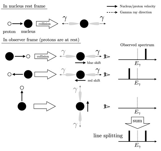
A schematic of line splitting. For simplicity, here we assume that the nuclei emit gamma rays in only two directions in the nucleus rest frame (top). In the observer frame (bottom), the observer can detect gamma rays from only the top two cases, which result in a split line profile.
The actual profile depends on the energy distributions of particles, the collisional cross-section, and the angular distribution of anisotropic gamma-ray emission at each energy. In the following section, we explain the procedure of calculating the prompt gamma-ray line shape with cross-section data and arbitrary particle energy distributions.
3 GAMMA-RAY LINE PROFILE CALCULATION
The reaction rate (R) per unit volume between two different particle species (here, we consider protons and nuclei) is described as (Weaver 1976)
where c is the speed of light, nA/p are the number densities of nuclei and protons in the observer frame, |$\boldsymbol {p}$| are the momentum vectors; |$f(\boldsymbol {p}_{\mathrm{A/\mathrm{p}}})$| are the momentum distributions of nuclei and protons in the observer frame; β and γ are the ratio of velocity to c and the Lorentz factor, respectively. The primed variables indicate those in the nucleus rest frame, and the non-primed variables indicate those in the observer frame. |$\sigma (\gamma ^{\prime }_{\mathrm{p}})$| is the collisional cross section for the excitation process. To calculate the line profile observed from a certain direction, we need to implement the anisotropy of the gamma-ray emission in the nucleus rest frame. To do so, we expand |$\sigma (\gamma ^{\prime }_{\mathrm{p}})$| as |$\displaystyle \int {\rm d}{\Omega _{\gamma }} \frac{{\rm d}\Omega ^{\prime }_{\gamma }}{{\rm d}\Omega _{\gamma }} \frac{{\rm d}\sigma \left(\gamma ^{\prime }_{\mathrm{p}},\theta ^{\prime }_{\gamma \mathrm{p}}\right)}{{\rm d}{\Omega ^{\prime }_{\gamma }}}$|. Note that Ωγ and |$\Omega ^{\prime }_{\gamma }$| are the solid angles in the observer and nucleus rest frames, respectively, and |$\theta ^{\prime }_{\gamma \mathrm{p}}$| is the angle between the gamma-ray and incoming proton directions in the nucleus rest frame. In Section 4, we will outline our data base used for |$\displaystyle \frac{{\rm d}\sigma \left(\gamma ^{\prime }_{\mathrm{p}}, \theta ^{\prime }_{\gamma \mathrm{p}}\right)}{{\rm d}\Omega ^{\prime }_{\gamma }}$|. As shown in Rybicki & Lightman (1986), we use
where θγA is the angle between the directions of the gamma ray and the incoming nucleus in the observer frame. Then, we can derive the photon emissivity in the observer’s direction
To compute the integral in equation (3), we adopt Monte Carlo integration by sampling |$\boldsymbol {p}_{\mathrm{p}}$| and |$\boldsymbol {p}_{\mathrm{A}}$|, and calculate the gamma-ray line profile numerically. The following is the procedure for the calculation.
- We sample the proton momentum, |$\boldsymbol {p}_{\mathrm{p}}$|, in the observer frame and calculate its energy Ep. The momentum distribution is assumed to be isotropic. In the case of thermalized protons, we sample the momentum component first and then calculate the energy so that the momentum components obey Maxwellian distribution.(4)$$\begin{eqnarray} f(p_{\mathrm{p},i}) \propto \displaystyle \exp \left(-\frac{p_{\mathrm{p},i}^2}{2 m_{\mathrm{p}} k T_{\mathrm{p}}}\right)~,i=1,2,3 \end{eqnarray}$$(5)$$\begin{eqnarray} E_{\mathrm{p}} = \sqrt{\left(\displaystyle \sum _{i=1,2,3}c^2 p_{\mathrm{p},i}^2\right) + m_\mathrm{p}^2 c^4}~. \end{eqnarray}$$
Note that mp and Tp are the proton mass and temperature, respectively; k is the Boltzmann constant.
- In the same way as step (i), we sample the nucleus momentum, |$\boldsymbol {p}_{\mathrm{A}}$| and calculate its energy EA. Its momentum distribution can be defined as(6)$$\begin{eqnarray} f(p_{\mathrm{A},i}) \propto \displaystyle \exp \left(-\frac{p_{\mathrm{A}, i}^2}{2 m_{\mathrm{A}} k T_{\mathrm{A}}}\right)~,i=1,2,3 \end{eqnarray}$$where mA(= A × mp) and TA are the nucleus mass and temperature, respectively. Note that A is the mass number of the nucleus.(7)$$\begin{eqnarray} E_{\mathrm{A}} = \sqrt{\left(\displaystyle \sum _{i=1,2,3}c^2 p_{\mathrm{A},i}^2\right) + m_{\mathrm{A}}^2 c^4}~, \end{eqnarray}$$
- We fix the gamma-ray direction as:(8)$$\begin{eqnarray} \boldsymbol {p}_{\gamma } \propto (0,0,1) \end{eqnarray}$$
Note that since the particle momentum distributions are isotropic here, the resulting gamma rays are also isotropic. Thus, the result does not depend on the observer’s direction. The (Doppler-shifted) gamma-ray energy Eγ will be determined at step (v).
- We convert |$(E_{\mathrm{p}}, \boldsymbol {p}_{\mathrm{p}})$| and |$(E_{\mathrm{\gamma }}, \boldsymbol {p}_{\gamma })$| into 4-momenta in the nucleus rest frame, |$(E^{\prime }_{\mathrm{p}}, \boldsymbol {p}^{\prime }_{\mathrm{p}})$| and |$(E^{\prime }_{\gamma }, \boldsymbol {p}^{\prime }_{\gamma })$| via Lorentz transformation. Then, we calculate a weight w, which we use to fill the gamma-ray energy of each event into a histogram.(9)$$\begin{eqnarray} & w = \displaystyle \frac{\gamma ^{\prime }_{\mathrm{p}}\beta ^{\prime }_{\mathrm{p}}}{\gamma _{\mathrm{p}}\gamma _{\mathrm{A}}}\frac{1}{\gamma _{\mathrm{A}}^2(1-\beta _{\mathrm{A}} \cos \theta _{\gamma \mathrm{A}})^2}\frac{{\rm d}\sigma \left(\gamma ^{\prime }_{\mathrm{p}}{, \ }\theta ^{\prime }_{\gamma \mathrm{p}}\right)}{{\rm d}{\Omega ^{\prime }_{\gamma }}} \end{eqnarray}$$(10)$$\begin{eqnarray} \displaystyle \gamma ^{\prime }_{\mathrm{p}} = \frac{p^{\mu }_{\mathrm{p}}p_{\mathrm{A}\mu }}{m_\mathrm{A} m_\mathrm{p} c^2} \end{eqnarray}$$
- We consider the gamma-ray energy in the nucleus rest frame, |$E^{\prime }_{\gamma }$|, to be fixed. For example, the energy of gamma rays from 12C is 4.44 MeV. Then, we again convert |$(E^{\prime }_{\gamma }, \boldsymbol {p}^{\prime }_{\gamma })$| into |$(E_{\gamma }, \boldsymbol {p}_{\gamma })$| to calculate the observed gamma-ray energy, Eγ.(11)$$\begin{eqnarray} \left(E^{\prime }_{\gamma }, c p^{\prime }_{1}, c p^{\prime }_{2}, c p^{\prime }_{3}\right) \longmapsto \left(E_{\gamma },0,0,E_{\gamma }\right) \end{eqnarray}$$
In this step, we ignore the energy shift due to the nucleus recoil after the proton collision. As discussed in section 2 of Kozlovsky et al. (1997), this recoil energy can affect the line shape if the nuclei are at rest and the protons have large energy. However, in this work, the nuclei have large velocities, and the Doppler shift by their motions is dominant. Thus, the recoil effect is insignificant under the conditions of this work. In Appendix B, we calculate the gamma-ray spectra considering the recoiling energy and evaluate this approximation. While the peak height in the spectra can be modified by a few per cent under special conditions, the basic features of the line profile are not affected by the recoil effect.
Finally, we fill Eγ calculated in step (v) into a histogram with the weight w.
We repeat the steps (i)–(iv) until sufficient statistics are accumulated and normalize the histogram by the number of Monte Carlo samples. Typically, 107 samples are used for each line profile calculation in this work.
In Section 5, following the above procedure, we will calculate the line gamma-ray emissivity per unit volume and density, defined as
We will also show the gamma-ray line profile, which can be derived as
4 CROSS-SECTION DATA
For our calculations, we describe our data-set for the angular distribution of the nuclear gamma-ray emission in the excited nucleus rest frame. The gamma-ray direction |$\mathrm{d}\Omega ^{\prime }_{\gamma }$| is determined relative to the momentum direction of an initial incoming proton. The differential cross section |$\displaystyle \frac{{\rm d}\sigma }{{\rm d}{\Omega ^{\prime }_{\gamma }}}$| is usually described well with Legendre polynomials
Note that here the cross-section is parametrized with the kinetic energy of protons in the nucleus rest frame |$E^{\prime }_{\mathrm{K,p}} (= E^{\prime }_{\mathrm{p}}-m_{\mathrm{p}}c^2)$|.
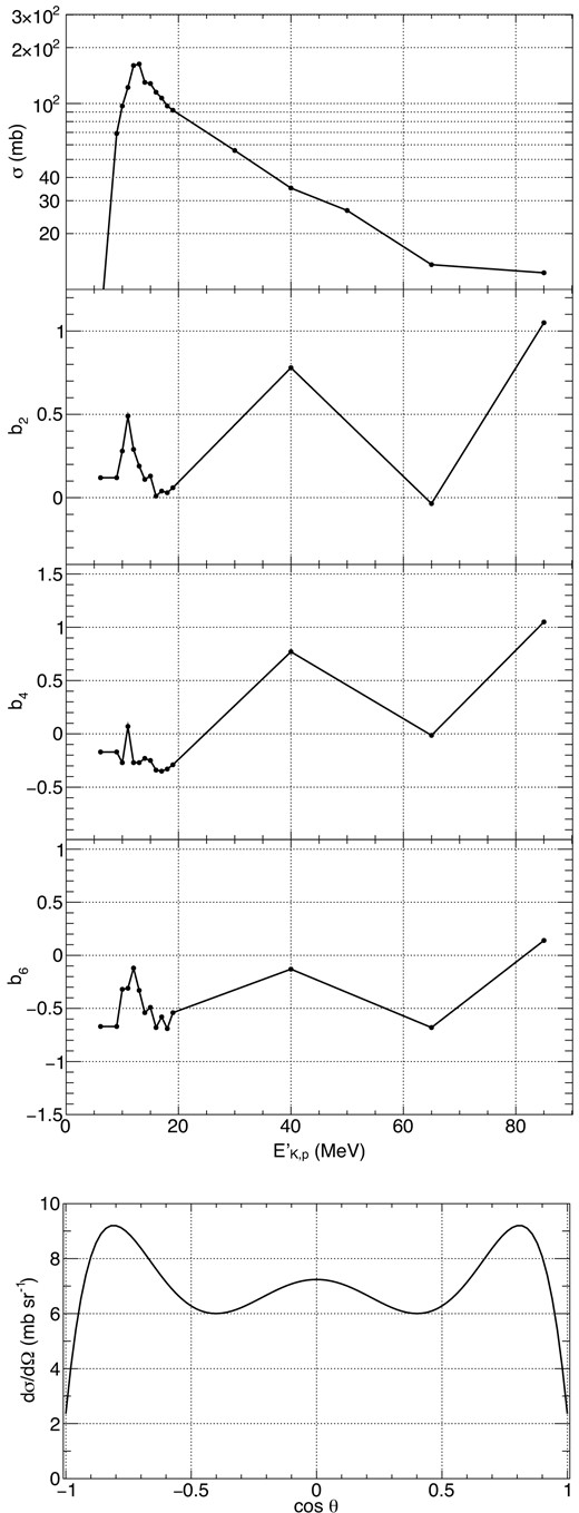
We extracted the cross-section data from several experimental works in nuclear physics (for 12C (p, pγ) 12C, Lang et al. (1987); Lesko et al. (1988); Kiener et al. (1998); Kiener, de Séréville & Tatischeff (2001), for 16O (p, pγ) 16O, Lang et al. (1987); Lesko et al. (1988); Kiener et al. (1998)). Fig. 2 shows the data we use for the 4.44 MeV gamma ray line from 12C interactions with protons. Fig. A1 shows those for 6.13 MeV gamma rays from 16O interactions with protons. Using the extracted data points, we calculate the functions b2l and the total cross section with linear interpolation.
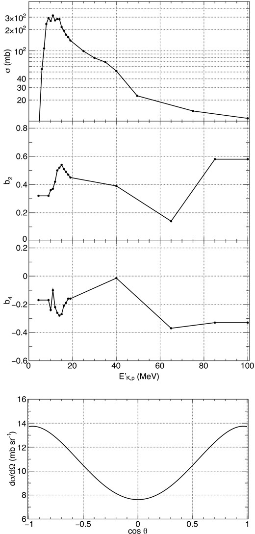
The cross-section data that we use for 4.44 MeV gamma-ray emission from 12C (p, pγ) 12C. The top is the total cross-section. The second and third are the coefficient b2 and b4, respectively. The bottom is the differential cross-section at |$E^{\prime }_{\mathrm{K,p}} = 20$| MeV as an example.
For 12C, due to the lack of experimental data, we assume that |$\sigma (E^{\prime }_{\mathrm{K,p}}=4.44~\mathrm{MeV}) = 0$| mb, and the functions b2, b4 between 4.44 and 9 MeV are the same as those measured at 9 MeV. We check the validity of this approximation in Appendix C. The cross-section at > 100 MeV is calculated as |$\displaystyle \left(E^{\prime }_{\mathrm{K,p}}/100~\mathrm{MeV}\right)^{-1} \times \sigma (E^{\prime }_{\mathrm{K,p}}=100~\mathrm{MeV})$|, and the coefficients are the same as those at 100 MeV. For 16O, also due to the lack of experimental data, we assume that |$\sigma (E^{\prime }_{\mathrm{K,p}}=6.13~\mathrm{MeV}) = 0$| mb, and the functions b2, b4, b6 between 6.13 and 9 MeV are the same as those measured at 9 MeV. The cross-section at >85 MeV is calculated as |$\displaystyle \left(E^{\prime }_{\mathrm{K,p}}/85~\mathrm{MeV}\right)^{-1} \times \sigma (E^{\prime }_{\mathrm{K,p}}=85~\mathrm{MeV})$|, and the coefficients are the same as those at 85 MeV.
It should be noted that the spallation process starts to dominate over the excitation above ∼20 MeV. We ran the nuclear reaction simulator TALYS (Koning, Hilaire & Duijvestijn 2005) and compared spallation cross-sections of Carbon with its de-excitation process. Fig. 3 shows that the cross-sections of the spallation processes producing 9B, 11C, and 8Be can be larger than the de-excitation process in a certain energy range. The spallation process could reduce the amount of Carbon and its line emissivity. On the other hand, the spallation of heavier nuclei would produce Carbon. For example, 16O (p, x γ4.4 MeV) 12C has a comparable cross-section of 16O (p, γ) 16O. This process can produce a 4.44 MeV gamma ray and increase the amount of Carbon after that. While it is beyond the scope of this paper, such a nuclear reaction network should be considered in the line modelling of certain astronomical sources.
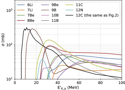
The cross-sections of the spallation processes of Carbon based on the TALYS code. The legend displays produced nuclei in the spallation processes. Here, only the processes with the maximum cross-section larger than 20 mb are shown.
5 RESULT
To focus on the basic properties of the gamma-ray line shape, we investigate it by changing the proton and nucleus temperatures, which are represented as kTp and kTA, respectively. Then, we will discuss its astrophysical applications in the following section. Here, we mainly show the line profile of 4.44 MeV due to 12C (p, pγ) 12C. Since basic features are found to be the same as those of 12C, the results for the 6.13 MeV gamma-ray line from 16O are shown in Appendix A.
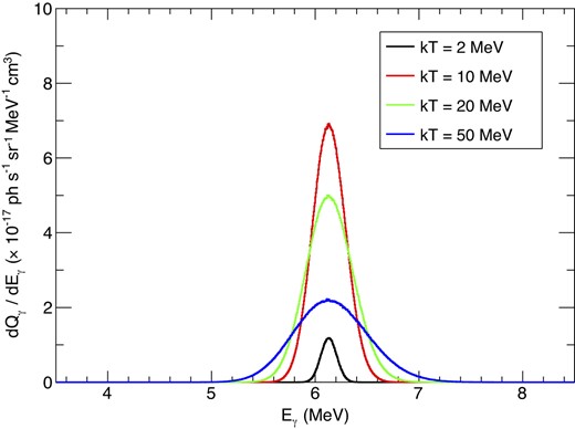
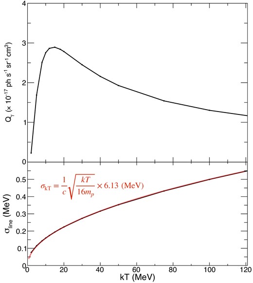
First, we calculate the line profile under equal temperatures, Tp and TA. We vary the common temperature from 2 to 50 MeV. Fig. 4 shows the calculated line profiles. In this case, the line profile is described well by a Gaussian, and the line splitting does not occur significantly. Fig. 5 shows the photon emissivity and the standard deviation σline of the line profile at each temperature. By tracing the cross-section of 12C (p, pγ) 12C, the emissivity obtains a maximum around 10 MeV. Also, the line width is consistent with the normal thermal Doppler broadening of
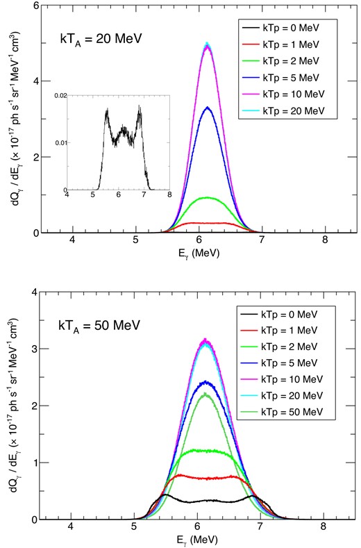
Next, as a typical case where the line splitting occurs, we show the line profile when TA is significantly higher than Tp. Fig. 6 shows the line profile by fixing kTA to 20 or 50 MeV, and changing kTp from 0 MeV to kTA. As seen clearly, when kTp is lower than a few MeV, the line profile is distorted from a Gaussian shape, and it has two peaks by reflecting the anisotropic gamma-ray emission in the nucleus rest frame as seen in Fig. 2. As kTp becomes larger than ∼5 MeV, the line profile is closer to a Gaussian-like shape again. This is because as far as the proton’s kinetic energy gets close to or less than the nucleus’s kinetic energy per nucleon, i.e. kTp ∼ kTA/A, the quantization axis of the gamma-ray emission is nearly parallel to the nucleus momentum direction in the observer frame, which causes the line splitting. However, when the proton’s kinetic energy becomes larger, the quantization axis is less aligned with the nucleus momentum direction and randomized in the observer frame. Then, the anisotropy is smeared out, and the line becomes Gaussian again. Considering that the mass number of carbon is 12, the maximum proton temperature that yields the line splitting can be estimated as ∼2 (=20/12) to ∼4 (=50/12) MeV, which is consistent with Fig. 6. In Appendix A, we also show the line profile of 6.13 MeV from 16O. Since the mass number of oxygen is 16, larger than carbon, the line splitting is smeared out at a lower proton temperature than for carbon (see Fig. A4).
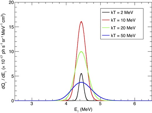
4.44 MeV gamma-ray line shape in the case that Tp = TA. Black: kTA = kTp = 2.0 MeV, Red: 10.0 MeV, Green: 20.0 MeV, Blue: 50.0 MeV.
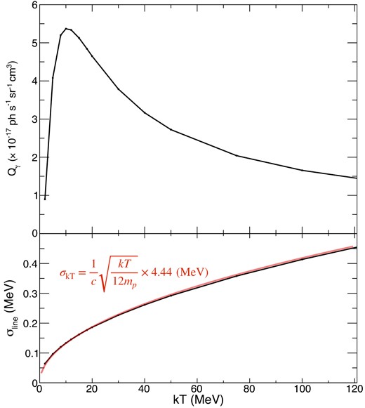
The dependence of the emissivity and the line width on the temperature in the case that Tp = TA. The top panel shows the gamma-ray emissivity depending on the temperature, and the bottom is the standard deviation of the line profile. The red line is the value expected from the normal thermal Doppler broadening.
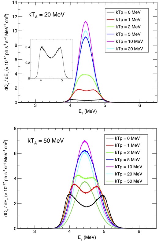
The line profile of 4.44 MeV gamma-ray lines with different proton temperatures. The nucleus temperature is fixed to 20 MeV (top) or 50 MeV (bottom). The line splitting is clearly seen when kTp is less than a few MeV. The inset in the top panel is a zoom of the line profile with kTp = 0 MeV.
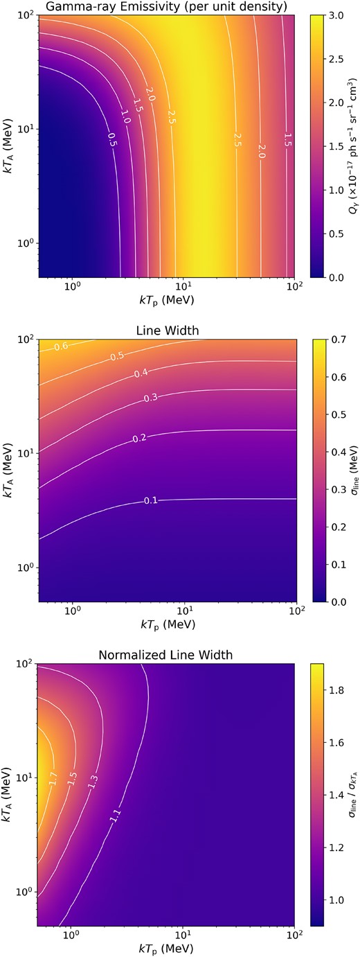
To make the dependence of the line profile on the hot plasma temperatures clear, we performed a parameter scan for Tp and TA. For each, we assigned values from 0.5 to 100 MeV. In addition to the gamma-ray emissivity Qγ and the line width σline, we also investigate the line width normalized by the normal thermal Doppler broadening width |$\sigma _{kT_{\mathrm{A}}}$| because it is a good indicator to know how much the line profile deviates from a Gaussian shape determined by the nucleus temperature. As shown in Fig. 5, |$\sigma _{\mathrm{line}}/\sigma _{kT_{\mathrm{A}}}$| is equal to one when the line splitting is not significant.
Fig. 7 shows Qγ, σline, and |$\sigma _{\mathrm{line}}/\sigma _{kT_{\mathrm{A}}}$| for different kTp and kTA. Here, we can derive two interesting properties of the line profile. One is that the gamma-ray emissivity and line width have apparently different dependence on kTp and kTA. The gamma-ray emissivity is mainly determined by the proton temperature. It is because to excite a nucleus by its own kinetic energy; it requires larger energy by a factor of its mass number than excitation by a proton. Especially for carbon, the nucleus kinetic energy needs to be more than 100 MeV to achieve the largest cross section at its rest frame. On the other hand, the line width is dominantly determined by the nucleus temperature, and it is less affected by the proton temperature. This is because the Doppler shift of the gamma-ray energy is determined by the nucleus motion. In principle, by combining Qγ and σline together, we can derive the temperatures for both the proton and nucleus observationally.
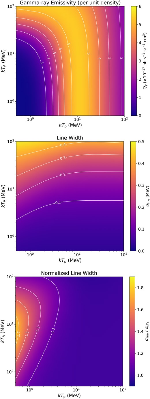
The gamma-ray emissivity of 4.44 MeV from 12C (p, pγ) 12C (top), line width (middle), and the normalized line width with different proton and nucleus temperatures (bottom).
The other is the condition in which the line splitting is significant. As shown at the bottom of Fig. 7, the normalized line width is larger than one when kTp is less than a few MeV, and it has a maximum at kTA ∼ 10 MeV. This means that the line-splitting effect can be significant only with a two-temperature plasma in which kTA ≫ kTp and kTp is less than a few MeV. Thus, if the line profile deviating significantly from a Gaussian profile is observed, it would be evidence that gamma rays are produced in such a two-temperature plasma.
We note that the peak height at the low-energy side of the line profile is higher than the high-energy side (see Fig. 6). It is because of a slightly longer tail at the high-energy side caused by the relativistic effect. When a gamma ray with the energy of Eγ is emitted from a nucleus with a velocity of β, the maximum red-/blue-shifts will be |$(\sqrt{(1 + \beta)/(1-\beta)}-1) \times E_\gamma$| and |$(1-\sqrt{(1 - \beta)/(1 + \beta)}) \times E_\gamma$|, respectively, with the averaged energy of |$E_\gamma /\sqrt{1-\beta ^2}$|. Thus, as β increases, the line becomes broader and shifts slightly towards the high-energy side. When one accumulates the line profiles produced by nuclei with different velocities in a Maxwellian distribution, the profile has a slightly longer energy tail at the high-energy side, resulting in a smaller peak height at this side.
6 DISCUSSION
In this work, we calculated the line profiles of gamma rays due to nuclei-proton collision. The interesting result is that the line is split when the temperature of the nuclei is much higher than that of the proton. This indicates that the line profile of the prompt gamma rays can be a smoking gun for MeV particles that are not fully thermalized in astrophysical systems.
6.1 Accreting black holes
One of the potential targets is the two-temperature accretion flows onto a compact star or a supermassive black hole. It is widely accepted that at low-mass accretion rates, the accretion flows become hot and optically thin because the energy advection is dominant and the radiation is inefficient (Shapiro, Lightman & Eardley 1976; Ichimaru 1977; Rees et al. 1982; Narayan & Yi 1994; Abramowicz et al. 1995).1 In contrast to the standard accretion disc model (Shakura & Sunyaev 1973), the electrons and the protons have different temperatures in this state because electrons radiate more efficiently than protons. Also, Coulomb coupling between electrons and protons is weak due to low densities. The solution is known as the advection-dominated accretion flows (Narayan & Yi 1994, 1995a, b). As a result, the proton temperature is close to the virial temperature in the hot accretion flow solutions, reaching ∼100 MeV × (r/rs)−1, where r is the distance from the central source and rs is the Schwarzschild radius (for a review, see Yuan & Narayan 2014).
For the same reason, the protons and nuclei can have different temperatures. For example, assuming the virial temperature, the free–fall time-scale becomes shorter than the proton-carbon thermal relaxation time-scale around r/rs = 10–100 when one assumes 0.01 Eddington luminosity (Spitzer 1962; Stepney 1983). Considering that the virial temperature is proportional to the particle mass, the temperature of the nuclei can be higher than that of the protons by a factor of their mass numbers. Furthermore, recent observations suggest the particle acceleration in the black hole corona (Inoue et al. 2019), and there is also a possibility that the particle energy distribution in the corona deviates from a Maxwellian distribution.
To demonstrate how the line profile depends on the particle energy distribution and the temperatures, here we assume several nuclei energy distributions and temperatures and outline some examples. Considering the hot accretion flow and the virial temperature, we set the average kinetic energy of nuclei to 12 times the kinetic energy of protons, as the gravitational energy release is proportional to the particle mass. The proton energy distribution is assumed to be a Maxwellian distribution. Fig. 8 shows the line profile with kTp = 2 MeV. Since the average energy as a function of temperature T is |$\frac{3}{2}kT$|, the nucleus kinetic energy is set to 36 MeV (=1.5 × 12 × 2.0 MeV). The red and green lines are the results with Gaussian energy distributions with a standard deviation (|$\sigma _{E_{\mathrm{A}}}$|) of 10 and 20 MeV, respectively. The blue line is the case when the energy distribution is Maxwellian. We note that the nucleus energy distributions in Fig. 8 have the same average energy, and these distributions trace the relaxation process from mono-energetic to thermal equilibrium. Our calculations show that we can disentangle the particles’ energy distributions by detailed observations of nuclear line profiles.
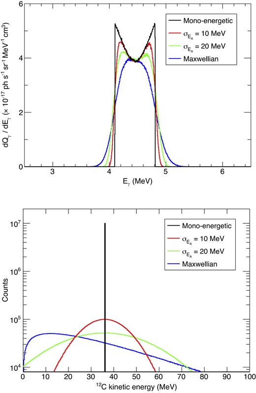
4.44 MeV gamma-ray line profiles from different nucleus energy distributions (top). The bottom panel shows the energy distribution of each case. Here, the averaged kinetic energy of Carbon is the same as 36 MeV over all cases. The proton is assumed to be Maxwellian with kTp of 2 MeV. The black line corresponds to the mono-energetic case. The red and green lines are the results of Gaussian energy distributions with |$\sigma _{E_k}$| of 10 and 20 MeV, respectively. In the blue lines, the Maxwellian distribution is assumed.
For a more detailed discussion, we need to account for the thermal distribution depending on the radial axis, other nuclear processes (see Section 4), and gravitational Doppler shift, etc., which is a subject for future work. Especially the radial dependence is critical to discuss the detectability of this effect because the observable line profile is the superposition of the lines at different radii. Since the protons and nuclei vary their temperatures with radius, the line-splitting effect could be suppressed and challenging to observe. However, the line gamma rays may be produced dominantly in the outer range of the corona (100–1000 rs) if the nuclear spallation reduces carbon’s fraction significantly as it reaches the centre (see fig. 3 of Kafexhiu, Aharonian & Barkov 2019b). Since the proton temperature is a few MeV at these radii, the line may still deviate from Gaussian in such cases. Also, the line profiles may be partially smeared by scattering processes very close to the central source because the Thomson optical depth is about ∼1 × (r/rs)−0.5 with 10−2 Eddington luminosity. Here, we adopt the solution shown in Narayan & Yi (1994) with αc1 = 0.05 and c3 = 0.5. We should also note that the continuum emission from the corona, e.g. the inverse-Compton scattering and thermal electron Bremsstrahlung (Inoue et al. 2019; Kafexhiu et al. 2019b), may overwhelm the line emission, causing less detectability.
We finally mention the line gamma-ray observations with future MeV gamma-ray satellites. Based on the spectral models by Kafexhiu et al. (2019a, b), the 4.44 MeV gamma-ray flux from a source at the distance of 2 kpc, such as Cygnus X-1, is estimated as 10−9–10−6 ph cm−2 s−1 depending on the assumed disk model and its parameters. The upcoming MeV gamma-ray satellite, the Compton Spectrometer and Imager will have a line sensitivity of a few × 10−6 ph cm−2 s−1 at 4.4 MeV (Tomsick et al. 2019). While it is not likely to observe the 4.4 MeV line, we would note that the upper bound of these fluxes is within reach if the observations are longer than the proposed and accepted 2-yr mission. Future MeV gamma-ray observations, e.g. AMEGO (McEnery et al. 2019) and GRAMS (Aramaki et al. 2020), are expected to have a better line sensitivity at 4.4 MeV, so that the brightest cases might be reached quicker.
6.2 Supernova remnants
The de-excitation gamma-ray lines are also used to infer the conditions of particle acceleration operated in supernova remnants (Liu, Yang & Aharonian 2021) and solar flares (Smith et al. 2003; Kiener et al. 2006). One of the delectable targets is Cassiopeia A. Summa, Elsässer & Mannheim (2011) modelled the nuclear de-excitation line spectrum from Cassiopeia A, predicting that the 4.44 and 6.13 MeV lines are close to the sensitivity limit of COMPTEL. Note that a new estimation was performed by Liu et al. 2023, showing that the line flux is lower than originally proposed. If the de-excitation lines are detected with future MeV missions, it can give information about low-energy cosmic rays, such as injection rate, gas density, and energy spectrum. As introduced in Section 1, the line-splitting effect can also occur in the non-thermal case if the accelerated nuclei collide with ambient protons (Bykov et al. 1996). In addition, there is a possibility that the two-temperature plasma is produced via the mass-proportional heating in the collisionless shock (Rakowski 2005; Ghavamian et al. 2013) though it is not clear whether it dominates over the non-thermal particles. Considering that the line profile depends on the particle energy distributions, as shown in Fig. 8, if the de-excitation lines are observed from supernova remnants, their line profile might be key observables to investigate the energy distribution of the produced MeV particles and the energy injection problem of low-energy cosmic rays.
7 CONCLUSION
In this paper, we have calculated the line profile of prompt gamma rays from 12C and 16O as examples considering the anisotropic gamma-ray emission in the nucleus rest frame. We found that the line splitting can take place in a hot two-temperature plasma in which the proton temperature is less than a few MeV, and the nucleus temperature is high enough to produce nuclear de-excitation gamma rays. In contrast, the gamma-ray line has a Gaussian-like shape when the proton temperature becomes higher and close to the nucleus temperature. Our results suggest that the profile of prompt gamma-ray lines can be a tool to probe for physical conditions in a very hot thermal plasma. It can be applied to investigate the particle distribution of nuclei and protons in the hot accretion flow around black holes, where protons and nuclei can have different temperatures of > few MeV. In addition, the particle injection of the acceleration process in supernova remnants might be studied by observations of gamma-ray line splitting. Considering the width of the split lines shown in Fig. 6 and A4 are 8 per cent and 2 per cent (1 σ), respectively, future MeV gamma-ray observations with an energy resolution of a few per cent at least are needed to enable such a new plasma diagnostics.
ACKNOWLEDGEMENTS
The authors would like to thank the anonymous referee, Karl Mannheim and Dmitry Khangulyan for useful comments. Hiroki Yoneda acknowledges support by the Bundesministerium für Wirtschaft und Energie via the Deutsches Zentrum für Luft- und Raumfahrt (DLR) under contract number 50 OO 2219. Tadayuki Takahashi acknowledges support from JSPS KAKENHI grant number 20H00153.
DATA AVAILABILITY
The cross-section data of the nuclear reactions used in this work are available in the articles listed in Section 4. The code developed for the line profile calculation in this work will be shared on reasonable request to the corresponding author.
Footnotes
Even at high-mass accretion rates (very high state), a hot but optically thick corona is considered to be formed (e.g. Kubota & Done 2004). If the protons and nuclei are heated to the MeV range, this state could also be a source of the de-excitation gamma-ray lines.
References
APPENDIX A: 6.13 MeV GAMMA RAY FROM 16O-P COLLISION
Using the cross-section data set shown in Fig. A1, We show our results in the case of 16O in Figs A2–A5. When the two temperatures are the same, the line has a Gaussian-like shape (Fig. A2), and the gamma-ray emissivity traces the cross-section (Fig. A3). These results are the same as those in the case of carbon. A difference is the line profile when the line splitting occurs. As shown in Fig. A4, the gamma-ray line can have three peaks because the differential cross-section has three peaks. Fig. A1 shows the differential cross section at E = 20 MeV. We observe the line splitting only when the proton energy is lower than a few MeV, as is the case of carbon (see the bottom panel of Fig. A5).
The cross-section data used for 6.13 MeV gamma-ray emission from 16O (p, pγ) 16O. The top is the total cross-section. The second, third, and fourth are the coefficient b2, b4, and b6, respectively. The bottom is the differential cross-section at |$E^{\prime }_\mathrm{K,p} = 20$| MeV, shown as an example.
6.13 MeV gamma-ray line profile assuming Tp = TA. Black: kTA = kTp = 2.0 MeV, Red: 10.0 MeV, Green: 20.0 MeV, and Blue: 50.0 MeV.
The dependence of the gamma-ray emissivity and the line width of 6.13 MeV gamma ray from 16O on the temperature, assuming Tp = TA. The top panel shows the gamma-ray emissivity depending on the temperature, and the bottom is the standard deviation of the line profile. The red line is the value expected from the normal thermal Doppler broadening.
The line profile of 6.13 MeV gamma-ray line with different proton temperatures. The nucleus temperature is fixed to 20 MeV (top) or 50 MeV (bottom). The inset in the top panel is a zoom of the line profile with kTp = 0 MeV.
The same as Fig. 7, but for 6.13 MeV from 16C (p, pγ) 16O.
APPENDIX B: THE EFFECT OF RECOIL ENERGY IN THE COLLISION
Kozlovsky et al. (1997) calculate the line profile, including the recoil energy in the case that the nuclei are at rest and protons have an energy of 23 MeV. In their approach, it is assumed that the anisotropic gamma-ray emission depends on θw, the angle between the direction of the gamma ray and the normal to the reaction plane in the centre-of-mass frame. However, it is difficult to apply this approach to our calculation, because there is no data to describe the anisotropic gamma-ray emission with θw in the energy range up to ∼100 MeV. They also consider that the recoiling nuclei are moving preferentially backward in the centre-of-mass frame (Ramaty et al. 1979), but these data are also lacking in the wide energy range.
Alternatively, we calculate the gamma-ray energy in the nucleus rest frame instead of fixing it as follows. In advance of the Monte Carlo calculation in Section 3, we calculate the gamma-ray energy distribution in the nucleus rest frame under assumptions that (1) the recoiling nuclei move isotropically in the centre-of-mass frame and (2) the gamma-ray emission is isotropic in the rest frame of an excited nucleus. We sample the excited nuclei and gamma-ray momenta and convert the gamma-ray energy into the nucleus rest frame. By repeating it, we obtain the gamma-ray energy distribution in the nucleus rest frame depending on the angle between the incoming proton and the gamma-ray direction. Then, at step (v) of the Monte Carlo calculation, we sample the gamma-ray energy in the nucleus rest frame from the pre-calculated gamma-ray energy distribution.
Fig. B1 shows an example of the line profile following the calculation considering the recoil effect. We can see that the recoil effect makes the line profile slightly narrower because the nuclei lose their kinetic energy by the excitation energy, and then the Doppler shift becomes smaller. Thus, the peak in the spectrum with the effect is higher than that without the effect. The difference of the peak height is |$\sim 5~{{\ \rm per\ cent}}$| in Fig. B1, where we assume that kTp = 0 MeV and kTA = 50 MeV. Though the recoil effect changes the line shape slightly, the line-splitting feature is kept even after including the effect. We should note that assumption (2) in the pre-calculation is inconsistent with the actual anisotropic gamma-ray distribution. To improve this point, we would need more experimental data about 12C (p, pγ) 12C, including the recoiling effect.
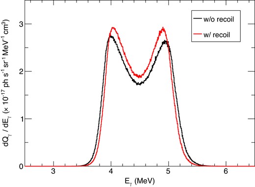
4.44 MeV line profile considering the effect of the recoil energy. The black and red lines correspond to the spectra without and with the recoil effect. Here kTp and kTA are set to 0 and 50 MeV, respectively.
APPENDIX C: VALIDITY OF THE APPROXIMATION OF THE CROSS-SECTION IN LOW ENERGY RANGE
For 12C (p, pγ) 12C, due to the lack of experimental data, we assumed that the coefficients b2, b4 between 4.44 and 9 MeV are the same as those measured at 9 MeV in the main text. However, we need to clarify whether this assumption is valid or not. We adopt a different approximation that the coefficients b2, b4 are zero at 4.44 MeV and compare the difference in the calculated line profiles. Note that with the new assumption, the gamma-ray emission is isotropic close to the threshold in the nuclei rest frame. Fig. C1 is the result with kTA = 50.0 MeV and kTp = 0.0 MeV. There is a difference of a few percent around the energy center, which is trivial and does not affect our discussion.

Comparison between the different approximations of the cross section in low energy range. Black: b2, b4 at 4.44 MeV are the same as those at 9 MeV, Red: b2, b4 are zeros at 4.44 MeV. Here, kTA = 50.0 MeV and kTp = 0.0 MeV are adopted.
