


ABSTRACT
Fresnel propagation of starlight after it passes through high altitude turbulence in the Earth’s atmosphere results in random fluctuations of the intensity at ground level, known as scintillation. This effect adds random noise to photometric measurements with ground-based optical telescopes. Spatial correlation of the intensity fluctuations means that the fractional photometric noise due to scintillation may be substantially smaller for a sparse array of small aperture telescopes than for a single large aperture of the same total area. Assuming that the photometric noise for each telescope is independent, averaging the light curves measured by N telescopes reduces the noise by a factor of |$\sqrt{N}$|. For example, for bright stars, the signal-to-noise ratio of a 2.54 m telescope can be achieved for an array of thirty 20 cm telescopes if the scintillation noise measured for each telescope is uncorrelated. In this paper, we present results from simulation and from observations at the Isaac Newton Telescope. These explore the impact that several parameters have on the measured correlation of the scintillation noise between neighbouring telescopes. We show that there is significant correlation between neighbouring telescopes with separations parallel to the wind direction of the dominant high altitude turbulent layer. We find that the telescopes in an array should be separated by at least twice their aperture diameter so that there is negligible correlation of the photometric noise. We discuss additional benefits of using sparse telescope arrays, including reduced cost and increased field of view.
1 INTRODUCTION
High-precision, time-resolved, ground-based photometry is critical for a wide range of astronomical applications. For example, for exoplanet photometry, it is vital for follow-up observations in order to verify the transit detection, to check for variations in the transit timings, and to improve the precision on transit parameters such as the period and depth (Collins et al. 2018). However, such ground-based observations are limited by the effects of the Earth’s atmosphere.
Arrays of small telescopes are in common use for exoplanet surveys such as the Wide Angle Search for Planets (SuperWASP) (Pollacco et al. 2006), the Multi-site All-Sky CAmeRA (MASCARA) (Lesage et al. 2014), and the Next Generation Transit Survey (NGTS; Chazelas et al. 2012). Such arrays are designed to observe large patches of the sky using small telescopes with very large fields of view (FOV). Many stars are observed simultaneously and automatic pipelines are used to search for periodic dips in their brightness.
However, another benefit of using such arrays has been recently exploited. By pointing all the telescopes in the array at a single bright target of interest and combining the photometry from all of the telescopes in the array, high signal-to-noise ratios (SNRs) can be achieved. For an array of N telescopes, averaging their light curves increases the SNR by a factor of |$\sqrt{N}$| if the photometric noise is uncorrelated. Simultaneous observations of WASP-166b by NGTS and the Transiting Exoplanet Survey Satellite (TESS; Ricker et al. 2014) show that ground-based sparse telescope arrays are capable of achieving SNRs comparable to those achieved in space (Bryant et al. 2020; Doyle et al. 2022).
Not only are arrays of small telescopes able to achieve high SNRs for bright stars, but they also have a much larger FOV than a large telescope. For example, each of the NGTS 20 cm telescopes has an FOV of 8 deg2. Hence, the likelihood of finding a bright comparison star in the field is significantly increased. Such bright comparison stars are necessary to minimize the addition of random noise fluctuations in differential photometry. As such, arrays of small telescopes could be used for ground based observations of exoplanet transits around bright stars with very high precision.
However, the |$\sqrt{N}$| increase in SNR of using an array of small telescopes is only achieved if the photometric noise from each telescope is independent. Any correlated noise between neighbouring telescopes would significantly reduce the improvement in the measured SNR. Noise sources such as the shot noise of the signal, readout noise, and the shot noise of the sky-background etc. are random and therefore will not be correlated between telescopes. However, for bright targets, the scintillation noise is likely to be the dominant noise source and may be correlated between neighbouring telescopes for long exposure times. This is because scintillation noise is produced by the propagation of the wavefront through high altitude turbulence, producing spatio-temporal intensity fluctuation patterns at the ground (Osborn et al. 2015b). Correlation between neighbouring apertures will depend on aperture size, turbulence strength, and the wind direction and exposure time, but can be substantial.
These effects all need to be considered when designing a telescope array to perform high-precision ground-based photometry. It has been shown for the NGTS telescope array that correlation of the photometric noise measured between neighbouring 20 cm telescopes separated by an order of ∼2 m is negligible (Bryant et al. 2020). Here, we consider telescope arrays with much smaller baselines which may be limited by such effects, for example, if the telescopes were mounted on a single mount, such as in the Gravitational-wave Optical Transient Observer (GOTO) array (Gompertz et al. 2020).
In this paper, we investigate the correlation of scintillation noise between neighbouring telescopes in an array for a range of parameters including wind direction, exposure time, and distance between telescopes. Results from both numerical simulation and observations at the Isaac Newton Telescope (INT) are presented and discussed, and we discuss several advantages of using sparse aperture arrays for photometric observations.
2 THEORY
2.1 Scintillation noise
Propagation through high altitude turbulence in the atmosphere produces spatial intensity fluctuations of starlight at ground level. These ‘flying shadow’ patterns change with time, both due to the turbulence moving with the wind and the turbulence itself evolving (Dravins et al. 1997), resulting in spatio-temporal intensity fluctuations.
The total integrated turbulence strength is often expressed by the Fried parameter, which is defined as:
where k is the wavenumber, γ is the zenith angle, h is the altitude of the turbulent layer, and |$C_{\mathrm{ \mathit{ n}}}^{2}(h)$| is the refractive index structure constant which is a measure of the vertical profile of the turbulence strength.
The characteristic size of the scintillation speckles is given by the radius of the first Fresnel zone, |$r_{\mathrm{ f}} = \sqrt{\lambda z}$|, where λ is the wavelength of the light and z is the propagation distance from the turbulent layer. Hence, as z increases, the characteristic spatial scale of the intensity fluctuations becomes larger (Osborn et al. 2015b).
The strength of the scintillation fluctuations is quantified using the scintillation index, which is given by the variance of the relative intensity fluctuations of the source:
where I is the intensity as a function of time and 〈 · 〉 represents an ensemble average. The scintillation rms fractional noise is then the square-root of the scintillation index.
The theoretical scintillation index is found by integrating the scintillation power spectrum for Kolmogorov turbulence (Kornilov 2012). For telescopes with D ≫ rf, the scintillation index for short exposures can be estimated as (Sasiela 2012):
where D is the telescope aperture.
For long exposure times, defined as t ≫ tcross, where t is the exposure time and tcross is the time taken for the layer to cross the telescope pupil, the scintillation index is given by (Sasiela 2012):
where α is the exponent of the airmass and V⊥(h) is the wind velocity profile. The value of α depends on the wind direction and will be −3 when the wind is transverse to the azimuthal angle of the star and −4 when it is longitudinal.
For bright stars, scintillation noise is the dominant noise source. The magnitude at which photon noise becomes dominant is dependent on the telescope aperture, with smaller telescopes becoming shot noise limited at lower magnitudes. For example, it has been found that scintillation dominates for stars of magnitude below V ∼ 10.1 mag for a 0.5 m telescope, and at V ∼ 11.7 mag for a 4.2 m telescope under median atmospheric conditions in La Palma (Föhring et al. 2019). Across the sky, there are close to 330 000 stars brighter than magnitude V = 10 (Hog et al. 2000) and therefore a significant number of stars to observe for which the SNR is limited by scintillation noise.
2.2 Sparse telescope arrays and scintillation-limited stars
For a bright star, the benefit of using an array of small telescopes over a single telescope of the same equivalent area for long exposure times can be determined by considering the SNR for both instruments.
To compare the two, consider a single telescope of diameter D and an array of N telescopes, each with diameter Dsub. Equating the two areas gives:
For a bright star where the noise is limited by scintillation noise, the SNR is proportional to:
where σI is the rms scintillation noise.
Hence, for long exposures on a single telescope of diameter D:
For an array of small telescopes where the photometric noise is uncorrelated between neighbouring telescopes, the scintillation index measured for the entire array is given by:
where |$\sigma _{\mathrm{ I}_\mathrm{sub}}^2$| is the scintillation index measured for a single telescope within the array of diameter Dsub.
Hence, for an array of telescopes where the photometric noise is uncorrelated:
Therefore, for long exposure times, the SNR of an array of small telescopes will be greater than the SNR measured by a single telescope of the same equivalent area. This is because SNRarray > SNRtel. Hence, an array of small telescopes can achieve the same SNR as a larger telescope with diameter:
for a fraction of the area of glass and hence a fraction of the cost. For example, the SNR of a 2.5 m telescope can be achieved with an array of thirty 20 cm telescopes.
For short exposure times, where |$\sigma _{\mathrm{ I}}^2 \propto D^{-7/3}$|, the SNR of a single telescope scales as D7/6. Therefore, using an array results in a lower SNR than using a single telescope of the same equivalent area. Therefore, the SNR benefit of using an array of small telescopes is only achieved for long exposure times where t ≫ tcross (for example, on the order of seconds rather than milliseconds).
2.3 Scintillation correlation
The scintillation noise can be correlated between two neighbouring telescopes. If we assume Taylor’s frozen flow hypothesis (Taylor 1938), then a high altitude layer of turbulence that is producing the scintillation noise will move a finite distance within the exposure time. As such, the spatial intensity fluctuations can translate from one pupil to the other. The degree of the correlation will be dependent on the averaging of the intensity fluctuations with the exposure time. An example of this spatio-temporal averaging for increasing exposure times is shown in Fig. 6. This leads to correlation between the scintillation noise for two apertures.
Several parameters affect the correlation of scintillation noise between neighbouring telescopes. These include:
wind direction of the high altitude turbulence relative to the separation vector of the telescopes
exposure time
wind speed of the high altitude turbulent layers
telescope diameter
distance between the telescopes
The correlation between the measurements of two telescopes is measured using the Pearson correlation coefficient, r, which is given by Benesty et al. (2009):
where x is the light curve measured from one telescope and y the light curve measured from another telescope.
The correlation can be calculated both through Monte Carlo simulation and analytically from weak perturbation scintillation theory (see Appendix A), both of which are presented here.
3 METHOD
The scintillation correlation measured between two telescopes is dependent on the parameters described above. The dependences of these parameters were investigated both in simulation and using INT telescope measurements. The method for each investigation is described below.
3.1 Simulation
To investigate the spatio-temporal correlation of scintillation in simulation, a Monte Carlo phase screen representation of the atmosphere was produced using the python package soapy (Reeves 2016). The phase screens were used with Fresnel propagation to simulate a scintillation pattern at ground level using the python package aotools (Townson et al. 2019). Small telescope pupils were cut out from this pattern and summed to give the integrated intensity for each pupil.
Turbulence profiles measured using a Scintillation Detection And Ranging (SCIDAR) turbulence profiler instrument (Shepherd et al. 2013) in La Palma and Paranal were used to produce accurate estimations for the strength and altitude of the turbulence layers above the telescope pupils in numerical simulation. The simulated atmospheres were updated and translated based on the turbulent profile wind velocities and directions in order to simulate the effect of the finite exposure time assuming Taylor’s frozen flow hypothesis. This was then repeated to produce a light curve with the appropriate temporal intensity fluctuations for each telescope.
The Pearson correlation coefficient was then measured between the neighbouring telescopes to measure the correlation of the intensity fluctuations due to scintillation. It should be noted that new phase screens were generated for each exposure, such that the temporal correlation measured was strictly dependent on the exposure time used.
We assume for all the simulations that the inner scale is much smaller than the spatial scale of the scintillation intensity fluctuations and that the outer scale is much larger than the size of the telescope apertures.
3.2 Telescope measurements
Measurements were made at the INT in La Palma, Spain by reimaging the telescope aperture plane on to a detector using a collimating lens. The detector used was a ZWO 1600 CMOS camera, which allowed the use of short exposures and high frame rates with relatively low readout noise. A SCIDAR instrument was also mounted on the telescope so that turbulence profile measurements could be interleaved with the photometric measurements. The SCIDAR data could then be used in numerical simulation to compare the on-sky photometric results to the simulation, for the prevailing turbulence and wind profile. The pupil-imager and SCIDAR turbulence profiler were mounted in parallel at the cassegrain focus with a folding mirror allowing us to switch between the two instruments.
We observed the scintillation pattern in the pupil plane in the V band for a range of exposure times. From these scintillation patterns, we could define an array of small sub-apertures equivalent to a sparse telescope array. These observations allowed us to measure the effect of a range of parameters on the scintillation correlation between the sub-apertures.
Data were obtained in two observing runs, in 2021 September and 2022 May. In the first observation a bright star, Aljanah, with magnitude V = 2.48 was selected as a suitable target. Pupil-plane images with exposure times of 0.01, 0.1, and 1 s were collected. Exposure times of more than 1 s would have saturated the detector. The second data run in 2022 May included longer exposure times of 2 and 3 s using the bright star Seginus, a magnitude V = 3.02 star.
3.3 Aperture size
To select a suitable aperture size for a sparse telescope array, careful consideration of the Optical Telescope Assembly (OTA) cost and the cost of the detectors is required.
The cost of a ground-based optical telescope scales with aperture size. Several models have been used to estimate the scaling of cost with aperture size. For example, van Belle, Meinel & Meinel (2004) estimated the scaling of cost with the ground OTA size as:
This relation is given for large telescopes. However, based on the price for commercial telescopes in the 20–100 cm range, a relation of D3 better reflects the cost scaling.
The correlation measured between pupils with separation also depends on telescope size. This is because the intensity fluctuations are averaged over a larger area and therefore measure larger scales which will be correlated over larger separations. Hence, large telescopes will need to be separated by larger distances.
There are two options for the sparse telescope array design. One is to have each telescope in the array on its own mount, as for the NGTS array. This gives the option of independent pointing of the telescopes, but will increase the cost and complexity. The second option is to have all the apertures mounted on to a single large mount, such as the GOTO array. Here, we consider this second option. In this case, the cost of the mount will scale more slowly with the number of telescopes.
The SNR increases with telescope size and the SNR of an array is proportional to SNR|$_\mathrm{tel}\sqrt{N}$| where SNRtel is the SNR of a single telescope in the array. Hence, for very small telescopes, we will need more telescopes in the array to reach the required overall SNR and therefore more detectors.
The telescope aperture used in an array should therefore be optimized to minimize the cost. Fig. 1 shows the estimated cost for a sparse telescope array as a function of the telescope diameter, assuming that an SNR for a scintillation-limited star observed with the INT is desired. The cost calculations assume a cost of £3k per camera and that the telescope cost scales as D3. The number of telescopes N required to match the SNR for the INT was calculated using equation (10), for a range of values of Dsub. For small telescopes, where a larger number of apertures is needed, the sparse array cost is dominated by the cost of the cameras, which decreases sharply with N and hence, aperture size. As the telescope size increases, the cost of the OTA starts to become more significant and a slow increase in array cost is seen. These two opposing parameters result in a shallow minimum.
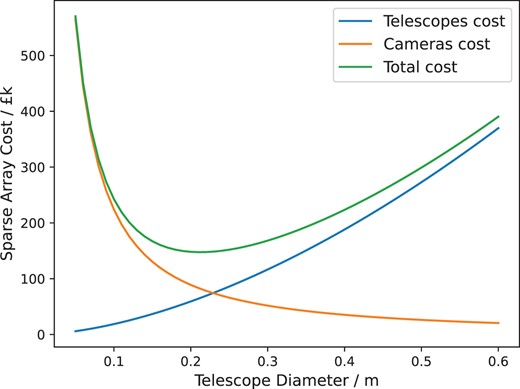
The cost of building a sparse telescope array that provides the same scintillation-limited SNR as the INT as a function of the diameter of the telescopes in the array. The cost for the telescopes and cameras are given assuming a cost of £3k per camera and assuming the telescope cost scales as D3.
Based on this figure, we propose the use of ∼20 cm telescopes as a suitable aperture size for building a sparse telescope array in terms of minimizing cost. Additionally, NGTS has already shown that an array of telescopes of this size can achieve SNRs equivalent to that of TESS observations (Bryant et al. 2020). Hence, an aperture size of 20 cm has been used for all the results given in Section 4.
4 RESULTS
In this section, we investigate the correlation of scintillation noise between neighbouring telescopes for a range of parameters. Results from both numerical simulations and our telescope measurements are presented.
4.1 Analytical and numerical simulation results
4.1.1 Wind direction
To investigate the significance of wind direction on the correlation of scintillation noise between two pupils, we modelled a turbulence profile consisting of a single layer at an altitude of 10 km and a wind velocity of 15 ms−1 with direction 0° for a 1 s exposure time. Two 20 cm telescopes were simulated. For all the results, the telescope pupils are initially superposed such that a correlation coefficient of r = 1 is measured. This overlapping of the telescope pupils is possible in simulation, but is not physically possible for real apertures. The pupils are then moved apart in a range of directions.
Fig. 2 shows a strong correlation between two telescopes separated parallel to the wind direction (0°), even at a separation of 1 m. As the telescopes are separated along directions away from the wind direction, the correlation drops significantly with distance. Telescopes that are positioned perpendicular to the wind direction are not correlated at all once the telescope pupils no longer overlap. The numerical simulation results closely follow the theoretical scintillation correlation, which are plotted as the solid lines.
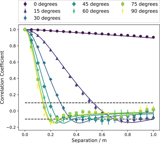
The correlation coefficient of the intensity fluctuations due to scintillation between two telescopes as a function of separation along the y-axis (north), which corresponds to 0° (see Fig. 3 for reference). A range of wind directions are plotted between 0° and 90°. The error bars represent the standard error in the Monte Carlo simulation, showing the statistical uncertainty. The theoretical scintillation correlation is plotted as the solid lines.
Hence, as expected, the wind direction of the high altitude turbulence is arguably the most significant parameter for the scintillation correlation measured between neighbouring telescopes for long exposure observations. Telescopes with baselines close to parallel to the wind direction, within ∼15°, will be highly correlated at short separations.
In reality, the atmosphere is not discrete and will typically have several significant turbulent layers moving in different directions, averaging out this effect. As such, we expect the measured correlation in scintillation noise between neighbouring telescopes to become negligible at much shorter separations if we assume a realistic turbulence profile rather than a single layer. However, sites will often have a prevailing wind direction for the high altitude turbulence due to atmospheric features such as the jet stream. In principle, telescope arrays could be designed with this in consideration by having longer baselines parallel to the prevailing wind direction.
4.1.2 Exposure time
Another significant factor affecting the correlation of scintillation noise between neighbouring telescopes is the exposure time used. The minimum distance required between neighbouring telescopes will depend on the distance that the high altitude turbulence has moved during an exposure time. For example, for a high altitude turbulent layer moving with a wind velocity of 30 ms−1, for a 1 s exposure time the turbulent layer, and therefore the spatial intensity fluctuations at the ground produced by this layer, will have moved 30 m, whereas for a 0.1 s exposure time it will have only moved 3 m. Hence, this will also be dependent on the wind speed of the high altitude turbulent layer.
A numerical simulation based on 15 different optical turbulence profiles from La Palma (Osborn et al. 2015a) was used to investigate how the correlation of scintillation noise between neighbouring telescopes varied with exposure time. These profiles were based on SCIDAR data collected in La Palma in 2015 and were produced using the hierarchical clustering method described by Farley et al. (2018). The median profile is given in Table. 1.
The median five layer SCIDAR profile measured at La Palma.
| Heights (m) | 0 | 250 | 3500 | 11 250 | 14 750 |
| Weights (r0 = 0.20 m) | 0.266 | 0.585 | 0.059 | 0.049 | 0.041 |
| Wind direction (degrees) | 159 | 236 | 238 | 262 | 143 |
| Wind speed (ms−1) | 6.8 | 8.7 | 10.6 | 12.9 | 10.5 |
| Heights (m) | 0 | 250 | 3500 | 11 250 | 14 750 |
| Weights (r0 = 0.20 m) | 0.266 | 0.585 | 0.059 | 0.049 | 0.041 |
| Wind direction (degrees) | 159 | 236 | 238 | 262 | 143 |
| Wind speed (ms−1) | 6.8 | 8.7 | 10.6 | 12.9 | 10.5 |
Four 20 cm apertures were used in simulation, two separated along the x-axis (parallel to the 90° and 270°directions) and two separated along the y-axis (parallel to the 0° and 180° directions). This is demonstrated in Fig. 3. This is the simplest configuration to explore a 2D array.
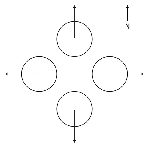
The geometry of the telescope positions relative to north used for the calculations shown in Fig. 4. The four telescopes begin entirely overlapped and are then moved in 2.5 cm steps in the directions indicated by arrows.
Fig. 4 shows the results of this simulation where the telescopes are (a) along the x-axis (parallel to the high altitude wind direction) and (b) along the y-axis (perpendicular to the high altitude wind direction). The numerical simulation results closely follow the theoretical correlation expected for each exposure time using the average SCIDAR turbulence profile for La Palma. For the shortest exposure time of 0.01 s, the scintillation correlation drops to zero as soon as the telescopes no longer overlap. As the exposure time increases, the measured correlation in the scintillation noise between the telescopes in (a) increases for all separations, i.e. for longer exposure times, a larger separation between neighbouring telescopes is needed for the scintillation noise to be uncorrelated. This is to be expected, as the atmospheric turbulence will have moved a larger distance over the exposure time, producing intensity correlations over larger spatial scales.
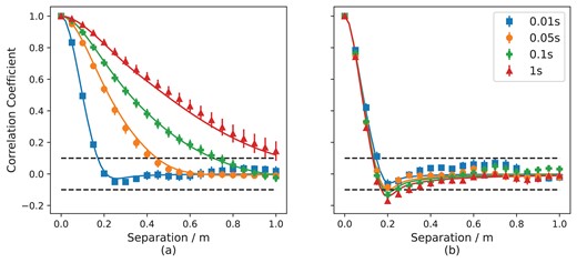
The average correlation coefficient of the intensity fluctuations due to scintillation between two telescopes as a function of separation (a) along the x-axis (parallel to the high altitude wind direction), and (b) along the y-axis (perpendicular to the high altitude wind direction) for the numerical simulation of 15 SCIDAR turbulence profiles measured in La Palma for a range of exposure times. The scatter in the correlation due to the variation in the turbulence profiles is represented by the standard error bars. The theoretical correlation coefficient for the average SCIDAR turbulence profile for La Palma is also plotted as solid lines.
However, if the telescopes are placed perpendicular to the wind direction, as shown in Fig. 4(b), the correlation of scintillation noise falls to zero once the telescopes no longer overlap for all of the exposure times used. There is small deviation between the simulated results and the theoretical scintillation correlation after 0.3 m, however the correlation measured in simulation is still negligible.
4.1.3 Telescope separation
A key question for the use of sparse telescope arrays is the minimum separation required between telescopes within a telescope array so as to reduce correlation of scintillation noise to a negligible level.
To determine the separation required between neighbouring telescopes, the array of four telescopes shown in Fig. 3 was tested in simulation using eighteen Paranal optical turbulence profiles produced using the hierarchical clustering of SCIDAR data. We explored the correlation of scintillation for 1 s exposures such that we expect the scintillation variance to be described by equation (4). The simulation was performed for five telescope aperture sizes of D = 15, 20, 28, 40, and 50 cm.
Fig. 5 shows the average SNR for a range of aperture sizes over the eighteen Paranal profiles for an array of four telescopes as a function of the separation in units of the aperture diameter, D. For all of the aperture sizes, the SNR levels off for separations larger than ∼2D. This suggests a centre-to-centre separation between neighbouring telescopes of at least 2D should be used.
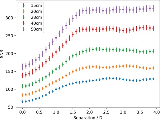
The average scintillation-limited SNR from simulation for an array of four telescopes with diameter D as a function of the centre-to-centre separation between them. The four telescopes are positioned as in Fig. 3. A range of telescope aperture sizes of D = 15, 20, 28, 40, and 50 cm are plotted. For all the aperture sizes, the SNR levels off for telescope separations greater than ∼2D.
It is possible that for longer exposure times (more than 10 s), a larger separation may be required. This is because for longer temporal averaging, larger spatial scales in the scintillation pattern will be more dominant. However, since the targets which are limited by scintillation noise are bright, very long exposure times cannot be used to avoid saturation. Therefore, this will rarely be a problem.
4.2 Telescope measurements
The results from Section 4.1 show how the wind direction, exposure time, and distance between neighbouring telescopes all affect the correlation of scintillation between two apertures. However, these simulations have limitations, such as the discrete number of turbulent layers that can be simulated and the assumption of frozen flow. Hence, telescope data were recorded to test this for the real atmosphere.
Examples of pupil-plane data for the INT with exposure times of 0.01, 0.1, and 1 s can be seen in Fig. 6. The variance in intensity across the pupil is very large for the 0.01 s data with the speckles clearly visible. For the 0.1 s data, streaks across the pupil can clearly be seen moving in the wind direction of the dominant high layer turbulence. For the 1 s frame, the pattern is averaged further and the intensity variance reduced.
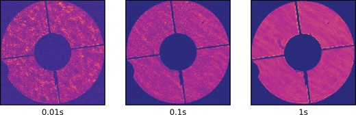
Example INT pupil-plane images for the 0.01, 0.1, and 1 s exposures. These show the spatio-temporal averaging of the scintillation pattern for increasing exposure time.
The average of all of the images recorded for each exposure time within a given observation run was used as a flat-field image. Some areas affected by dust and small fibres in the optical path, which are visible in the 1 s image, were avoided entirely in the data analysis as it could affect the measured scintillation correlation.
4.2.1 SCIDAR turbulence profile
The stereo-SCIDAR instrument was used to measure the turbulence profile above the INT in between pupil-plane data collections. The median of 12 profiles measured between 22:00 and 23:00 on 2021 September 19 is given in Table 2. This profile was grouped into five layers using the Optimal Grouping method (Saxenhuber et al. 2017).
The median five layer SCIDAR profile measured between 22:00 and 23:00 on 2021 September 19.
| Heights | 0 | 211 | 7175 | 12 028 | 13 927 |
| Weights (r0 = 0.16 m) | 0.619 | 0.240 | 0.029 | 0.072 | 0.040 |
| Wind direction | 130 | 106 | 92 | 84 | 64 |
| Wind speed | 4.4 | 2.1 | 15.7 | 20.7 | 16.4 |
| Heights | 0 | 211 | 7175 | 12 028 | 13 927 |
| Weights (r0 = 0.16 m) | 0.619 | 0.240 | 0.029 | 0.072 | 0.040 |
| Wind direction | 130 | 106 | 92 | 84 | 64 |
| Wind speed | 4.4 | 2.1 | 15.7 | 20.7 | 16.4 |
The SCIDAR profile measured is typical for La Palma with a strong ground layer and another strong layer at an altitude of approximately ∼12 km. It should be noted that measuring the wind direction and speed for the turbulent layers is challenging and can only be performed by tracking strong features over time. As such, wind speed and direction measurements are only available for the dominant layers.
4.2.2 Exposure time, wind direction, and aperture separation
A Monte Carlo algorithm was implemented to investigate the importance of wind direction, exposure time, and telescope separation. This worked by randomly selecting start locations within the INT pupil-plane images from which it was possible to offset by at least 0.75 m without leaving the limits of the pupil area or intersecting the shadow of the secondary mirror and its supports. From the pupil-plane image, two sub-pupils were cut out and summed to measure the intensity within each pupil. One pupil remained stationary at the start location and the second pupil would then be moved incrementally in the given direction with the intensity being recorded at each location.
In this way, the scintillation correlation could be recorded in a range of directions for a range of telescope separations. The Monte Carlo algorithm was run ten times for each direction to ensure the average result was not affected by any flat-field irregularities, for example, due to dust within the reimaging optics. This method was repeated for the data collected for each exposure time.
Data packets comprising 200 frames were collected. Fifteen 0.01 s packets, eleven 0.1 s packets, and seventeen 1 s packets were collected between 23:00 and 00:30 on the night of 2021 September 19. The results using the pupil-plane data for 0.01, 0.1, and 1 s exposure times are shown in Figs 7(a), (b), and (c), respectively. For very short exposure times, the measured scintillation correlation drops to zero as soon as the pupils are not overlapping, even along the wind direction. Whereas, for the long exposure data, the measured scintillation correlation along the wind direction increases at larger separations. The increased correlation is seen for orientations within approximately 15° of the aperture separations. Hence, the on-sky data agree with the simulation results from Figs 2 and 4 for both wind direction and exposure time.
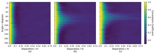
The measured correlation between two 20 cm apertures as a function of angle and separation for the INT pupil-plane images with an exposure of (a) 0.01 s, (b) 0.1 s, and (c) 1 s.
The profile given in Table 2 was used in a Monte Carlo simulation to compare the scintillation correlation results to the on-sky data for the 1 s exposure time. Fig. 8 shows the simulated results. Comparing to Fig. 7, it is clear that the simulation overestimates the measured scintillation noise correlation between the two telescope pupils at large separations. This is to be expected as the simulation assumes Taylor’s frozen flow hypothesis and approximates the atmosphere as discrete with only five layers, whereas in reality the atmospheric turbulence profile is continuous.
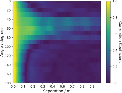
The measured correlation between two 20 cm apertures as a function of angle and separation for a numerical simulation using the SCIDAR profile given in Table 2 and a 1 s exposure time.
Based on these results, we can see that in most cases neighbouring telescopes within an array will be uncorrelated. Only pairs of telescopes with baselines close to parallel to the wind direction will exhibit significant correlation of the scintillation noise. This drops significantly with separation and is almost negligible after ∼40 cm. Based on the results in this section, an array of 20 cm within a sparse array should be separated by at least 40 cm from centre to centre. This is in agreement with the results from numerical simulation shown in Fig. 5 in Section 4.1.3 which suggests a separation of 2D is required.
4.2.3 Optical sparse arrays
To test the relation between the number of telescopes in an array and the resulting photometric SNR, multiple 20 cm pupils were cut from the pupil-plane data to create an array, each separated by 40 cm. An example is shown in Fig. 9 where the telescope pupils used in the array are the black circles. The intensity for each telescope is measured by summing the flux within each circle. The array was rotated and shifted such that the maximum number of pupils can fit within the INT pupil image whilst avoiding the secondary obscuration and any irregularities in the field. The presence of the secondary mirror obscuration limited the number of pupils that could be placed within the array and meant that the average distance between the pupils was slightly larger than 40 cm.
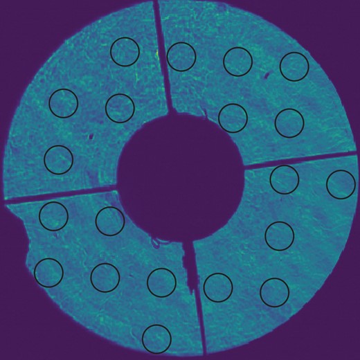
Example of using the INT pupil-plane images to estimate the SNR for an array, where each black circle represents a telescope pupil in the array. The intensity for each telescope is measured by summing the flux within each circle.
The overall photometric SNR for the whole array found by averaging the intensity over all the telescopes was then plotted against the summed area of the telescopes in the array. In addition, a single telescope of the same summed area as the array was cut from the pupil-plane image and the SNR recorded to allow a direct comparison.
Data packets comprising 200 pupil-plane images were recorded with the INT in 2022 May for a range of exposure times. Thirteen 0.1 s packets, five 1 s, three 2 s and two 3 s packets were collected between 22:50 and 00:00 on the night of 2022 May 15. Fewer long exposure data packets could be collected due to time constraints.
Fig. 10 shows the average normalized SNR as a function of the total area of the telescope array, as well as the results for a single telescope of the same area, for a range of exposure times. The SNR for each exposure time was normalized using the average SNR value for a single 20 cm aperture such that the shape of the trends could be easily compared between the different exposure times. The error bars represents the standard error over the data packets. The theoretical mean SNR for the telescope array and monolithic telescope described by equations (9) and (7) respectively are also plotted. For all the exposure times, the SNR measured for the array of telescopes exceeds the SNR measured for the monolithic telescope of equivalent area and all scale as expected from equation (9). This implies there is negligible correlation of scintillation noise between the pupils.
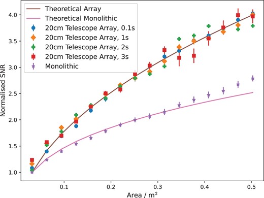
The average normalized SNR for a range of exposure times over all the data packets as a function of the total area for an array of telescopes. The average normalized SNR for a monolithic telescope is also plotted as a function of its area. The theoretical SNR for the telescope array and monolithic telescope described by equations (9) and (7) respectively are also plotted. The SNR for each exposure time was normalized using the average SNR value for a single 20 cm aperture. The error bars represent the standard error over the data packets.
If however we consider the short exposure regime, for a bright star, the SNR of the telescope array is worse than for a single telescope of the same area, as shown in Fig. 11. This is to be expected due to the aperture size dependence on the scintillation index for short exposure times given in equation (3) as discussed in Section 2.2. Therefore, the improvement in the SNR for using a telescope array over a single telescope of equal area is only beneficial for long exposure times where t ≫ tcross. Fortunately, for most applications such as exoplanet follow-up observations, typical exposure times (>1 s) fall within this regime.
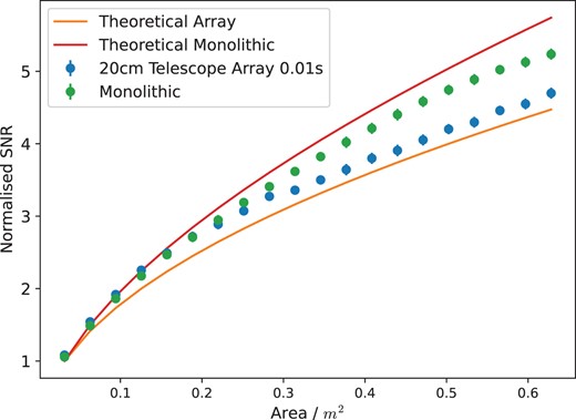
The average SNR for an array of 20 cm telescopes in an array as a function of the area of the telescope array and the SNR of a single monolithic pupil as a function of telescope area for a 0.01 s exposure time. The average normalized SNR for a monolithic telescope is also plotted as a function of its area. The theoretical SNR for the telescope array and monolithic telescope are also plotted. The SNR for each exposure time was normalized using the average SNR value for a single 20 cm aperture. The error bars represent the standard error over the data packets.
4.3 Sparse telescope array exoplanet transit simulation
In this section, we present a simulated exoplanet transit light curve demonstrating the SNR improvement that can be achieved for thirty 20 cm telescopes in an array compared to a single 1 m telescope. Based on equations (4) and (9), an array of thirty 20 cm telescopes (which has a total glass area of 1 m) should have an SNR equivalent to a single telescope of aperture diameter 2.54 m.
An exoplanet transit light curve of WASP-8b, a hot Jupiter exoplanet that orbits a star similar to the sun with magnitude V = 9.9 (Borsato et al. 2021), was simulated. A single layer turbulence profile was used with a wind speed of 15 ms−1, an r0 = 0.15 m, and using an exposure time of 10 s. It was assumed that the photometry was limited by scintillation noise and that the scintillation noise between the telescopes was uncorrelated.
Fig. 12 shows the results of a Monte Carlo simulation for a transit of WASP-8b for an array of thirty 20 cm telescopes and for a single 1 m telescope. The standard error for the wings of the transit is plotted in the bottom right-hand corner for the array, a 1 m telescope and for a 2.54 m telescope. Based on these error bars, the array can achieve a noise-to-signal ratio (NSR) 50 per cent smaller than a 1 m telescope, an NSR equivalent to a single telescope with a diameter of 2.54 m.
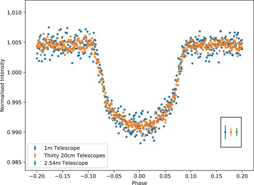
Simulated exoplanet transit light curve of WASP-8b for thirty 20 cm telescopes in an array and for a single 1 m telescope. The standard error for the wings of the transit is plotted in the bottom right-hand corner for the array and for a 1 m telescope. In addition, the standard error for a 2.54 m telescope has been added for comparison.
Since the uncertainty of the fitted astrophysical parameters of the exoplanet transit scales linearly with the scintillation noise, with a gradient in the range of 0.68–0.80 (Föhring et al. 2019), using a sparse array of thirty 20 cm telescopes will result in a reduction in the uncertainty of the exoplanet transit parameters by approximately 40 per cent when compared with a single telescope of the same equivalent area.
From Fig. 1, the cost of the telescope array is approximately £150k, assuming the individual 20 cm OTAs would have a typical cost of £2k and £3k per camera. The cost of a 2.54 m telescope would be substantially higher at approximately £2 million. Hence, for bright stars, exoplanet observations with SNRs equivalent to a 2.54 m telescope could be achieved for approximately a tenth of the price by building an array instead.
In addition, the probability of finding a suitable comparison star within the FOV is much higher for the array of small telescopes. If we consider telescopes with a focal ratio of 10, using the same detector with a pixel width of 3.8 µm, then the area of the FOV for a single 20 cm and 2.54 m telescope will be 0.19 deg2 and 0.001 deg2, respectively.
Fig. 13 shows the probability of finding a star of a given V-band magnitude within the FOV of the 20 cm and 2.54 m telescopes. The vertical blue and orange lines on Fig. 13 indicate the magnitude below which the photometric noise is dominated by scintillation noise for each telescope (Osborn et al. 2015b). The 20 cm telescope has an FOV 190 times larger than the 2.54 m telescope and therefore has a much higher likelihood of finding a bright comparison star within the FOV.
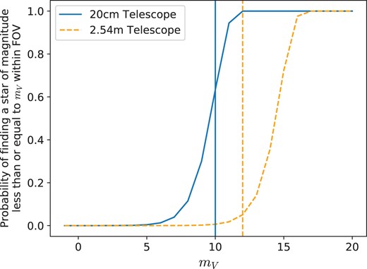
The probability of finding a star of V ≤ mV in the FOV of a 20 cm and 2.54 m telescope. The vertical lines represent the magnitude at which the photometric noise is dominated by scintillation noise for each telescope.
The shorter focal length also means that the requirements for the pointing and tracking is reduced, significantly reducing the cost of the array. If we require the images to fall on the same pixels to reduce systematic errors, then good tracking will be needed. However, the use of defocusing or diffusers (Stefansson et al. 2017) with bright stars would reduce this requirement. In addition, if instrumental systematic errors are independent for the telescopes in the array, then the errors will average.
5 DISCUSSION AND CONCLUSIONS
For bright stars for which photometric noise is limited by scintillation noise, arrays of small telescopes have several potential benefits. For long exposure times, an array of N telescopes of diameter Dsub can achieve an SNR equivalent to a single telescope of diameter equal to N3/4Dsub. However, this is only achieved if the scintillation noise is uncorrelated between the telescopes in the array.
We have investigated the impact of parameters including wind direction, aperture size, and the exposure time on the correlation of scintillation noise between neighbouring telescopes. The strong agreement between the theoretical scintillation correlation and the Monte Carlo simulation results provides confidence in the results. It was found in simulation that the scintillation correlation between two telescopes parallel to the high altitude turbulence wind direction was high, even over large physical separations. For on-sky measurements, the correlation between the telescopes reduced more quickly. This is most likely because the simulation has only a few discrete turbulent layers and assumes frozen flow. In reality, the turbulence profile is more continuous and will evolve such that Taylor’s frozen flow is not an exact description. Hence, in reality, the scintillation correlation reduces to negligible levels at smaller telescope separations than expected from simulation.
However, in both cases, the measured scintillation correlation fell to near negligible values for a centre-to-centre separation of ∼2D between telescopes. We have shown using pupil-plane imaging at the INT that the overall SNR for an array of telescopes separated by ∼2D is |$\propto \sqrt{N}$|. Hence, we recommend that in practice, a telescope separation of at least 2D should be used for a sparse telescope array.
One of the most significant benefits for using a telescope array over a larger monolithic telescope is that the same SNR can be reached using a fraction of the glass area and thus also at a fraction of the cost. For example, using thirty 20 cm telescopes can achieve the equivalent SNR as the INT, a 2.54 m telescope for a tenth of the cost. In addition, small telescopes have a much larger FOV, therefore increasing the probability of finding a suitable bright comparison star.
The increase in SNR for a telescope array compared to a single telescope of the same area is only achieved for long exposure times. For short exposure times, on the order of a few milliseconds, there is no benefit to using a telescope array over a single large telescope. In addition, an increase in SNR is only achieved for bright stars where the photometric noise is dominated by scintillation. In this regime, the SNR of a single telescope scales with the telescope aperture as D2/3 whilst the SNR for a sparse telescope array scales with D. For a fainter star where the observation is shot noise limited, the SNR scales linearly with the aperture diameter. Hence, an array of telescopes would perform as well as a single telescope of identical area. Therefore, there is no SNR benefit to using an array over a single telescope for faint, shot noise limited stars. However, the advantages of the reduced cost and increased FOV remain.
ACKNOWLEDGEMENTS
This work was supported by the Science and Technology Facilities Council(ST/N50404X/1) and (ST/T506047/1). The authors would like to thank the Isaac Newton Group (ING) for supporting their observations at the Isaac Newton Telescope. KH and JO acknowledge support from UK Research and Innovation (Future Leaders Fellowship MR/S035338/1).
This research made use of python including numpy and scipy (van der Walt, Colbert & Varoquaux 2011), matplotlib (Hunter 2007), astropy, a community-developed core python package for astronomy (The Astropy Collaboration 2013), and the python AO utility library aotools (Townson et al. 2019).
DATA AVAILABILITY
Please contact the lead author for data availability.
References
APPENDIX A: THEORETICAL SCINTILLATION CORRELATION BETWEEN SPATIALLY SEPARATED APERTURES
From the definition of scintillation index in equation (2), for an array of two apertures with intensities I1 and I2 we have
If we assume both apertures are the same size, with 〈I1〉 = 〈I2〉 = 1, the term 〈I1 + I2〉2 = 2〈I〉2 + 2〈I〉2 = 4. Developing the numerator above, we obtain
where we have assumed |$\langle I_1^2 \rangle = \langle I_2^2 \rangle = \langle I^2 \rangle$|. Using the definition of the single aperture scintillation index we can substitute |$\langle \mathrm{ \mathit{ I}}^2 \rangle = \sigma _\mathrm{ I}^2 + 1$|, obtaining
Finally, we note that the normalized intensity I = 1 + δI, where δI is a random variable with 0 mean and variance |$\sigma _\mathrm{ I}^2$|. This allows us to write
where 〈δI1δI2〉 represents the covariance of scintillation in each aperture. We then obtain
which reduces to equation (8) in the case of 〈δI1δI2〉 = 0, i.e. no covariance between apertures. The covariance is therefore given as
From standard scintillation theory in the weak perturbation limit (Roddier 1981), the scintillation index including aperture averaging and exposure time effects can be obtained by the following integral over altitude and the two dimensional Fourier plane
where h represents altitude and f the two dimensional spatial frequency vector with f = |f|. The quantity Φϕ(h, f) is the turbulent phase spatial power spectrum for a turbulent layer at altitude h, and the sin 2 filter describes the effect of propagation to the ground. The sinc2 filter represents temporal averaging of the scintillation according to the wind vector vwind(h) for the layer at altitude h (Tokovinin 2002).
The aperture filter |$A({\it{f}})=|\mathcal {F}(P({\it{r}}))|^2$| is the square modulus of the Fourier transform of the pupil function P(r). For a single circular aperture this is given by
where J1 is the Bessel function of the first kind and D is the single aperture diameter. For two apertures separated by the vector Δ, we use the convolution theorem of the Fourier transform with two Dirac delta functions to obtain
where the factor of 1/4 arises from normalization of the two apertures. For the computation of covariance, combining equations (A6), (A7), and (A9) we obtain
which can be straightforwardly numerically integrated. The correlation, r(Δ), is then obtained by normalizing the covariance
It should also be noted that the scintillation index for an arbitrary N-aperture array may be directly calculated by integrating equation (A7) using the aperture filter
where the Δi are the spatial coordinates of the centre of each aperture of the array.
