


ABSTRACT
This is the second paper of the Mapping Nearby Galaxies at Apache Point Observatory (MaNGA) Dynamics and stellar Population (DynPop) series, which analyses the global stellar population, radial gradients, and non-parametric star-formation history of ∼10K galaxies from the MaNGA Survey final data release 17 and relates them with dynamical properties of galaxies. We confirm the correlation between the stellar population properties and the stellar velocity dispersion σe, but also find that younger galaxies are more metal-poor at fixed σe. Stellar age, metallicity, and mass-to-light ratio (M*/L) all decrease with increasing galaxy rotation, while their radial gradients become more negative (i.e. lower value at the outskirts). The exception is the slow rotators, which also appear to have significantly negative metallicity gradients, confirming the mass–metallicity gradient correlation. Massive disc galaxies in the green valley, on the |$(\sigma _{\rm e},\rm age)$| plane, show the most negative age and metallicity gradients, consistent with their old central bulges surrounded by young star-forming discs and metal-poor gas accretion. Galaxies with high σe, steep total mass-density slope, low dark matter fraction, high M*/L, and high metallicity have the highest star-formation rate at earlier times, and are currently quenched. We also discover a population of low-mass star-forming galaxies with low rotation but physically distinct from the massive slow rotators. A catalogue of these stellar population properties is provided publicly.
1 INTRODUCTION
Galaxies trace the large-scale structure in the Universe. Thus, their evolution with cosmic time is a key question for the study of the Universe. Evolution of galaxies is a complicated process, involving multiple components, including stars, gas, dark matter, active galactic nuclei, as well as the surrounding environments of the galaxies. Therefore, although many efforts have been made to understand the evolution of galaxies, it still remains one of the great challenges of modern astrophysics (see Somerville & Davé 2015; Naab & Ostriker 2017 for review).
Stellar population of galaxies encodes the information of galaxy mass assembly and chemical enrichment histories, which is thus essential for understanding the evolution of galaxies. Early studies typically made use of galaxy colour to classify different stellar populations and chemical compositions in galaxies (see Baade & Gaposchkin 1963; Tinsley 1980 for review), which, however, suffers from the degeneracies between age and metallicity (e.g. Worthey 1994), as well as between the star-formation history (SFH) and dust attenuation effect (e.g. Silva et al. 1998; Devriendt, Guiderdoni & Sadat 1999; Pozzetti & Mannucci 2000). The latter is even stronger for late-type galaxies (LTGs), which have more dust than early-type galaxies (ETGs).
To break the degeneracies, people try to fit some spectral absorption features that have different sensitivities on age, metallicity, and dust attenuation effect, e.g. the Lick system (Worthey 1994), using a linear combination of single stellar population (SSP) templates. SSP models combine stellar evolution theory in the form of an initial mass function (IMF; e.g. Salpeter 1955; Kroupa 2001; Chabrier 2003), stellar tracks and/or isochrones (e.g. Bruzual & Charlot 1993; Vazdekis et al. 1996; Conroy, Gunn & White 2009), and stellar libraries that are either empirical or theoretical or a combination (e.g. Maraston 1998; Walcher et al. 2009; Vazdekis et al. 2010, 2016; Conroy et al. 2018) to predict the spectrum of a stellar population with given age and metallicity. Another way to study the stellar population of galaxies is the full-spectrum fitting, instead of fitting specific absorption features. Existing fitting methods include Penalized Pixel-Fitting method (ppxf, Cappellari & Emsellem 2004; Cappellari 2017, 2023), starlight (Cid Fernandes et al. 2005), stecmap (Ocvirk et al. 2006a, b), vespa (Tojeiro et al. 2007), fit3D (Sánchez et al. 2016a, b; Lacerda et al. 2022), and firefly (Wilkinson et al. 2017).
With the methods aforementioned, many efforts have been made to study the stellar population and SFH of galaxies. Kauffmann et al. (2003) used the |$4000\ \mathring{\rm A}$| break strength and the Balmer absorption-line index HδA to study the SFHs, dust attenuation, and stellar masses of |$\sim\!120\, 000$| galaxies from the Sloan Digital Sky Survey (SDSS; Stoughton et al. 2002). Gallazzi et al. (2005) studied the connection among metallicity, age, and stellar mass in nearby galaxies with the similar method but applies a Bayesian approach. Thomas et al. (2010) obtained luminosity-weighted ages, metallicities, and α/Fe ratios from the Lick absorption-line indices for 3360 ETGs and found that the scaling relations between galaxy stellar population properties and dynamical properties (i.e. galaxy mass and velocity dispersion) are not sensitive to environment densities. More recently, Scholz-Díaz, Martín-Navarro & Falcón-Barroso (2023) made use of the absorption feature method to study the dependence of SFHs of galaxies on halo mass. With full-spectrum fitting, Cappellari et al. (2013b) and McDermid et al. (2015) studied the correlation between stellar population properties and dynamical properties of 260 ETGs in ATLAS|$^{3\rm D}$| (Cappellari et al. 2011) and found that stellar population properties show systematic variation on the mass–size plane, roughly along the direction of velocity dispersion of galaxies. Scott et al. (2017) extended this study to ∼1300 galaxies from the SAMI survey (Bryant et al. 2015) and Li et al. (2018) to ∼2000 galaxies with different morphologies (including both ETGs and LTGs) in Mapping Nearby Galaxies at Apache Point Observatory (MaNGA; Bundy et al. 2015) and also found similar trends.
Besides, with the development of large-scale integral field unit (IFU) surveys, such as SAURON (Bacon et al. 2001; de Zeeuw et al. 2002), ATLAS3D (Cappellari et al. 2011), CALIFA (Sánchez et al. 2012), SAMI (Bryant et al. 2015), and MaNGA (Bundy et al. 2015), one can, not only study the global stellar population properties, but also analyse the spatially resolved stellar population properties, with which the population profiles and gradients can be studied. For example, Kuntschner et al. (2010) analysed the absorption-line strength maps of 48 ETGs from the SAURON survey to study their stellar population gradients and found that the age gradient depends on dynamical mass, with the scatter being smaller at the low-mass end. García-Benito et al. (2017) studied the gradient of mass-weighted age of 661 galaxies with various morphologies from the CALIFA survey and found that negative mass-weighted age gradient is seen for all the samples investigated and the gradient increases (becomes flatter) with increasing stellar mass surface density. Goddard et al. (2017) applied the stellar population analysis to a representative sample of 721 galaxies from the MaNGA survey and concluded that galaxy mass is the main driver of the variation of stellar population gradients among different galaxies; the galaxy environment seems to have no obvious influence on the stellar population gradients, consistent with the findings of Zheng et al. (2017) with 1105 galaxies from the MaNGA survey and Santucci et al. (2020) with 96 passive central galaxies and their satellite counterparts from the SAMI survey. The mass dependence of stellar population radial profiles (gradients) is also seen in Belfiore et al. (2018), in which low-mass star-forming galaxies appear to have nearly flat specific star-formation rate (sSFR) profiles, while the more massive star-forming galaxies show a significant decrease in sSFR at the galaxy centre. With a larger sample of ∼2000 galaxies with various morphologies from MaNGA, Li et al. (2018) studied the distributions of stellar population gradients on the mass–size plane and found that the variation of stellar population gradients have complicated dependence on dynamical parameters of galaxies and their variation cannot be accurately captured by mass alone. Interested readers are referred to Sánchez (2020) for a review on the spatially resolved spectroscopic properties of galaxies (see section 4.7 for stellar population gradients).
With the end of the MaNGA survey, the spatially resolved spectra of over 10 000 unique nearby galaxies have been successfully obtained (Abdurro’uf et al. 2022). Neumann et al. (2022) (known as the firefly catalogue) and Sánchez et al. (2022) (known as the pipe3d catalogue) have provided the catalogues of both the global and spatially resolved stellar population properties for the full sample of MaNGA, which have been widely used in many studies on the analyses of stellar content of galaxies. For example, Barrera-Ballesteros et al. (2022) studied the stellar population radial profiles of |$\sim\!10\, 000$| MaNGA galaxies with the pypipe3d analysis pipeline (Lacerda et al. 2022). Boardman et al. (2022, 2023) studied the driving factors of gas metallicity gradients, combining the pipe3d catalogue and the gas metallicity maps derived with the MaNGA Data Analysis Pipeline (DAP, Belfiore et al. 2019; Westfall et al. 2019) emission line fluxes with the Marino et al. (2013) calibrator. Apart from using the existing catalogues, Bernardi et al. (2023a, b) studied the influence of stellar IMF on the estimates of stellar population properties (e.g. age, metallicity, and stellar mass-to-light ratio) and further the influence on estimating the half-stellar mass radius using the full MaNGA sample.
With a series of papers of the MaNGA Dynamics and stellar Population (DynPop) project, we aim to not only provide catalogues of dynamical and stellar population properties for the final sample of the MaNGA survey (|$\sim\!10\, 000$| nearby galaxies; Abdurro’uf et al. 2022) as a legacy product, but also to study the formation and evolution of galaxies with the combination of the dynamical and stellar population properties. In Paper I (Zhu et al. 2023b), we performed the Jeans Anisotropic Modelling (JAM; Cappellari 2008, 2020) on the full sample of MaNGA survey and obtained their quality-assessed dynamical properties. This work is the second paper of the MaNGA DynPop series. The goal of this work is to provide a catalogue of stellar population properties, gradients, and SFH properties for all the |$\sim\!10\, 000$| MaNGA galaxies. With these properties, we will also make analyses of the scaling relations of stellar populations and the correlation of population gradients and SFH versus structural and dynamical properties of galaxies. The readers are also referred to Paper III (Zhu et al. 2023a) for a study of multiple dynamical scaling relations of these galaxies, and Paper IV (Wang et al. 2023) for a study of the density profiles from galaxies to clusters, combining the stellar dynamical modelling and weak lensing.
The paper is organized as follows. In Section 2, we describe the MaNGA data used for this work (Section 2.1), the structural and dynamical properties of MaNGA galaxies (Section 2.2), and stellar population synthesis (SPS) method (Section 2.3). In Section 3, we present the one-dimensional (1D) correlation between global stellar population properties and velocity dispersion of galaxies (Section 3.1) and the variation of global stellar population properties in 2D planes (Section 3.2). Section 4 presents the correlation between stellar population profiles/gradients and other galaxy properties. The analysis of SFHs of MaNGA galaxies is given in Section 5. Finally, we summarize our findings in Section 6. Throughout the paper, we assume a flat Universe with Ωm = 0.307 and |$H_0 = 67.7\, \mathrm{km\, s^{-1}\, Mpc^{-1}}$| (Planck Collaboration XIII 2016).
2 DATA AND METHODOLOGY
2.1 MaNGA data product
MaNGA (Bundy et al. 2015) is currently the largest IFU spectroscope survey in the world, targeting |$\sim\!10\, 000$| nearby galaxies in the redshift range 0.01 < z < 0.15 (Yan et al. 2016b; Wake et al. 2017). The spectra cover a simultaneous wavelength range from |$3600$| to |$10\, 300\ \mathring{\rm A}$|, with a spectral resolution R ∼ 2000 (Drory et al. 2015). They are produced by the Data Reduction Pipeline (DRP; Law et al. 2016), which calibrates and reduces the raw data from MaNGA observation. The observation covers a spatial range from 1.5 to 2.5Re (where Re is the effective radius of galaxies) for each observed galaxy, conducting the ‘Primary + ’ and ‘Secondary’ samples (|$\sim\!67{{\ \rm per\,cent}}$| and |$\sim\!33{{\ \rm per\,cent}}$|, respectively; Bundy et al. 2015). Readers are referred to the following papers for more details on the MaNGA instrumentation (Drory et al. 2015), observing strategy (Law et al. 2015), spectrophotometric calibration (Smee et al. 2013; Yan et al. 2016a), and survey execution and initial data quality (Yan et al. 2016b). The MaNGA project is now finished and the complete data have been released (Abdurro’uf et al. 2022).
2.2 Structural and dynamical properties of galaxies
In this work, we mainly use the structural and dynamical properties of MaNGA galaxies from the first paper of this series (Paper I; Zhu et al. 2023b). In Paper I, we perform the JAM (Cappellari 2008, 2020) to the complete sample of MaNGA survey (|$\sim\!10\, 000$| nearby galaxies) and obtain their quality-assessed dynamical and structural properties, using the python version of JAM, JamPy.1 Below, we briefly introduce the parameters used in this work:
Ellipticity (ϵ): ϵ is the ellipticity of the elliptical half-light isophotes of the galaxies, obtained with find_galaxy routine in the python software, MgeFit2 by Cappellari (2002).
Galaxy size (|$R_{\rm e}^{\rm maj}$| and Re): |$R_{\rm e}^{\rm maj}$| is the semimajor axis of the elliptical half-light isophotes of the galaxies. Re satisfies |$\pi R_{\rm e}^2 = A$|, where A is the area of the elliptical half-light isophotes of galaxies. The galaxy sizes here are derived from the Multi-Gaussian Expansion (MGE) models (Emsellem, Monnet & Bacon 1994; Cappellari 2002) with the MgeFit software and are scaled by a factor of 1.35 to approximately match the popular galaxy sizes obtained from extrapolated photometry (see fig. 7 of Cappellari et al. 2013b).
- Galaxy velocity dispersion (σe): σe used here is calculated as the square-root of the luminosity-weighted average second moments of the velocity within the elliptical half-light isophote, defined aswhere Vk and σk are the mean line-of-sight velocity and dispersion in the kth IFU spaxel, respectively, and Fk is the flux in the kth spaxel. The summation goes over all the spaxels within the elliptical half-light isophote. Velocities and dispersion here are obtained by the MaNGA DAP (Belfiore et al. 2019; Westfall et al. 2019).(1)$$\begin{eqnarray} \sigma _{\rm e} = \sqrt{\frac{\sum _{k}F_{k}(V_{k}^2+\sigma _{k}^2)}{\sum _{k}F_{k}}}, \end{eqnarray}$$
- Spin parameter of galaxies (|$\lambda _{R_{\rm e}}$|): |$\lambda _{R_{\rm e}}$| is calculated as (Emsellem et al. 2007)(2)$$\begin{eqnarray} \lambda _{R_{\rm e}} = \frac{\sum _{k} F_k R_k\left|V_k\right|}{\sum _{k} F_k R_k \sqrt{V_k^2+\sigma _k^2}}, \end{eqnarray}$$
where Rk is the distance to the galaxy centre of kth spaxel. The other parameters are the same as equation (1). |$\lambda _{R_{\rm e}}$| is also calculated within the elliptical half-light isophotes of galaxies.
Galaxy r-band luminosity (Lr): Lr is the total SDSS r-band (Stoughton et al. 2002) luminosity, derived by analytically integrating the MGE parametrization of the galaxy SDSS r-band surface brightness distribution.
Galaxy mass (MJAM): MJAM provides an approximation to the total stellar mass of a galaxy derived from stellar dynamics. More specifically, MJAM ≡ Lr × (M/Lr)e, where (M/Lr)e is the total (including stars and dark matter) mass-to-light ratio within a sphere of radius r = Re from JAM. Given the generally small amounts of dark matter within Re, which is typically on the order of 10 per cent (see Paper III of this series), the total (M/Lr)e is close to the stellar mass-to-light ratio (M*/Lr)e for most galaxies. For this reason, MJAM ≈ Lr × (M*/Lr)e = M*. When dark matter becomes important, MJAM will overestimate M*, but for most galaxies one expects the dynamical measurement to be more robust than the mass inferred from stellar population, due to the influence of possible IMF variations among galaxies (van Dokkum & Conroy 2010; Cappellari et al. 2012; Li et al. 2017), as well as due to the effect of outshining, which makes it difficult to measure accurate masses of very young stellar populations (e.g. Maraston et al. 2010; Sorba & Sawicki 2015). The readers are referred to Smith (2020) for a review on IMF variations. For the reasons above, we adopt MJAM as the estimator of the galaxies stellar masses.
Galaxy total mass density slope (γtot): γtot is the mass-weighted total density slope within a sphere of effective radius (e.g. Dutton & Treu 2014; Li et al. 2019). The total density slope of galaxies is obtained by JAM.
Dark matter fraction (fDM): fDM used here is calculated as the dark matter fraction within a sphere of radius Re.
We note here that Paper I provides structural and dynamical properties of MaNGA galaxies from multiple JAM models with different assumptions on dark haloes and velocity ellipsoids. In this work, we take the total mass-to-light ratio, (M/Lr)e, from the JAM with a mass-follows-light model (i.e. the total galaxy mass is assumed to be proportional to the r-band luminosity of the galaxy) and a cylindrical-aligned velocity ellipsoid (Cappellari 2008), following the practice of Cappellari et al. (2013b). The total mass-to-light ratio in this model is set to be constant across the whole single galaxy and thus does not vary with the aperture size. The other JAM-related parameters (i.e. the total mass density slope and the dark matter fraction) are from the results of the JAM modelling with a constant stellar mass-to-light ratio, a spherical NFW (Navarro, Frenk & White 1997) dark halo, and a cylindrical-aligned velocity ellipsoid. We note here that the total mass-to-light ratio (or equivalently, MJAM) and the total mass density slope of galaxies would not change too much under various model assumptions, while the dark matter fraction changes dramatically with model assumptions. Our readers are referred to Paper I for more details on the discrepancies among different models. In addition, Paper I provides quality flags (|$\rm Qual$|) of all the 10 000 galaxies for the users with different purposes. Galaxies with |$\rm Qual=-1$| are those with unreliable/irregular kinematic maps, for which no kinematic properties can be trusted. Thus, in this work, we only take the galaxies with |$\rm Qual\ \gt\ {-}1$| (9147 unique galaxies out of 10 296 observations) to make analyses, in order to balance the data reliability and the sample size. The readers are referred to table 2 of Paper I for more details of data quality flags. We note, however, the above selection criterion is only applied when making statistical analyses, while the catalogue of stellar population properties and SFHs will contain all the 10 296 observations, among which 10 010 are unique galaxies.
2.3 Stellar population synthesis
2.3.1 Stellar libraries
In this study, we make use of the ppxf3 by Cappellari & Emsellem (2004) as upgraded in Cappellari (2017, 2023) to carry out the spectrum fitting. For comparison, we adopt three different single stellar population (SSP) models in this work:
The fsps4 model (Conroy et al. 2009; Conroy & Gunn 2010), which allows one to compute SSP models for a specified set of parameters (e.g. age, metallicity, IMF, etc.). In this work, we adopt 43 ages linearly spaced by 0.1 dex in |$\lg \rm age$| (yr) from 6 to 10.2 (i.e. from 1 Myr to 15.85 Gyr) and nine equally spaced metallicities [Z/H] = [−1.75, −1.5, −1.25, −1, −0.75, −0.5, −0.25, 0, 0.25].
The galaxev5 model, which provides a Fortran code (version 2020) to generate SSP models under a set of parameters as fsps. Here, we adopt the same age grid as fsps, while use a different metallicity grid with [Z/H] = [−2.34, −1.74, −0.73, −0.42, 0, 0.47].
The miles-based (Sánchez-Blázquez et al. 2006) SPS models of Vazdekis et al. (2010)6 (hereafter, the Vazdekis model), for which we adopt 25 linearly spaced |$\lg \rm age$| from 7.8 to 10.2, with the same step of 0.1 dex (i.e. from 63.1 Myr to 15.85 Gyr) and seven metallicities [Z/H] = [-2.32, −1.71, −1.31, −0.71, −0.40, 0, 0.22].
For all models, we adopt the same Salpeter (1955) IMF. We use the default Padova (Girardi et al. 2000; Marigo et al. 2008) evolutionary isochrone for the Vazdekis and galaxev models and the MIST isochrones (Choi et al. 2016) for the fsps model. To better illustrate the age and metallicity grids of each library, we present them in Fig. 1. In general, the galaxev and fsps models have the same age and similar metallicity range, while the Vazdekis model lacks low-age templates and has a lower metallicity boundary. In this work, we take the fsps model as our default setting and only make comparisons between the models when necessary (see Section 3.1 for explanations).
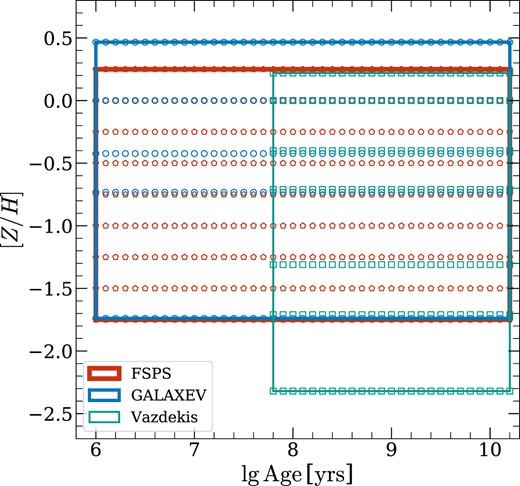
Sketch map of age and metallicity grids of the fsps (red), galaxev (blue), and Vazdekis (green) models.
2.3.2 Fitting procedure
Photons emitted by a distant galaxy will experience two dust extinction processes: one from the dust of the Milky Way (MW), and the other from the distant galaxy itself. The second effect is theoretically stronger for edge-on LTGs. In this work, we consider these two processes separately. First, we correct the MW dust attenuation effect using a Calzetti et al. (2000) reddening curve, with the |$\rm \mathit{E}(\mathit{B}-\mathit{V})$| values of MW for the corresponding sky regions of our samples from the NASA Sloan Atlas (NSA) catalogue7 (Blanton et al. 2011). After correcting the dust attenuation effect of MW, the corrected spectra are taken as the input for ppxf fitting. The dust attenuation effect from the target galaxy is then evaluated by setting the dust keyword in the software, assuming a two-parameter attenuation curve, i.e. (AV, δ), where AV is the attenuation of the spectrum at |$\lambda = 5500\ \mathring{\rm A}$| (V band) and δ is the ultraviolet (UV) slope of the spectrum (see Cappellari 2023, section 3.7 for details).
To better demonstrate this process, we present Fig. 2, where we show the spectra of two example galaxies (both are the stacked spectra within half-light isophotes; a star-forming LTG and a passive ETG) at different stages of this fitting process: The observed spectra from DRP data cube are shown by the black curves; after correcting the MW dust attenuation effect, we get the blue curves, which are then taken as the input spectra for ppxf fitting.
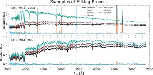
Two examples (LTG: 7961–12703; ETG: 7961–1902) of spectra at different fitting stages. In each panel, the black curve is the observed spectrum (including stellar continuum and gas emission lines) obtained from MaNGA DRP data cube; the blue curve is the observed spectrum with the MW dust attenuation effect corrected, which is taken as the input of ppxf fitting (including stellar continuum and gas emission lines); the red curve is the best-fitting spectrum given by ppxf, with the solid curve representing the best-fitting stellar continuum and the dashed curve representing the best-fitting gas emission lines; the green curve is the intrinsic spectrum of the galaxy, which is derived by the combination of best-fitting templates (including stellar and gas emission line templates, indicating by solid and dashed curves, respectively) with velocity and dispersion convolved (no dust attenuation). The orange curve is the best-fitting gas-only spectrum and the cyan diamonds are the fitting residuals. The grey-shaded region is the region of sky lines, which is masked and not fitted.
During the spectrum fitting, we simultaneously fit the stellar populations and the kinematics of the stellar continuum and the gas emission lines by assuming a Gaussian distribution and free velocities and dispersions of the stellar component and the gas emission lines. The gas emission lines included in our fitting are listed in Belfiore et al. (2019, see their table 1), which are taken as the default setting of the ppxf software. During the fitting, we do not fit the multiplicative polynomials by setting mdegree = -1 in the ppxf software. We emphasize here that in our analysis, we conducted a simultaneously fitting of kinematics and stellar population properties, rather than fitting them separately. We confirm that this simultaneous fitting procedure had minimal impact on the stellar population properties. The fitting range in this work is |$3550{-}7400\ \mathring{\rm A}$|. For all stellar population properties, we do not adopt regularization (i.e. regul = 0), while for SFH-related parameters, we adopt regul = 100 to obtain smoother template weight distributions (see Section 5 for more details).
As shown in Fig. 2, the red curves are the best-fitting results of the given spectra, which are the linear combinations of the best-fitting templates with best-fitting velocities and velocity dispersions convolved and the best-fitting dust attenuation effect (of the investigated galaxy) considered. The green curves are the best-fitting ‘intrinsic’ spectra of the distant galaxies, without undergoing any dust extinction processes. As can be clearly seen, the LTG has obviously stronger gas emission (the orange curves) and more significant dust attenuation effect from its own dust than the ETG, which is consistent with our previous understanding that LTGs typically have more dust than ETGs.
To quantitatively evaluate the dust attenuation effect, we show, in Fig. 3, the distribution of AV on the |$(\epsilon , \lambda _{R_{\rm e}})$| plane (see Section 2.2 for definitions of these two parameters). The |$(\epsilon , \lambda _{R_{\rm e}})$| plane is usually used to classify slow- and fast-rotators in ETGs (e.g. Emsellem et al. 2007, 2011; Fogarty et al. 2015; see Cappellari 2016 for a review). Here, however, we plot both ETGs and LTGs to investigate their dust attenuation variation on the |$(\epsilon ,\lambda _{R_{\rm e}})$| plane as a continuous sample. Before plotting, we make use of the python implementation (Cappellari et al. 2013b) of the 2D Locally Weighted Regression (loess;8 Cleveland & Devlin 1988) method to obtain a smoothed distribution of the colour-coding values. A small smoothing parameter frac = 0.1 is adopted for all these kinds of figures (including Figs 6, 7, 8, 9, 12, 13, 14, 15, and 18) in this work. As can be seen, dust attenuation effect show obvious variation on the plane. First, the slow-rotating galaxies (those within the region of black lines) appear to experience weaker dust attenuation effect (i.e. lower AV value) than the fast-rotating galaxies. At fixed ϵ, AV increases (i.e. dust attenuation effect getting stronger) significantly from the low |$\lambda _{R_{\rm e}}$| region (most of which are quenched ellipticals) to the high |$\lambda _{R_{\rm e}}$| region (most of which are star-forming disc galaxies). Besides, galaxies show obvious increasing trend of AV (i.e. dust attenuation effect getting stronger) from the face-on view to the edge-on view of the galaxies (i.e. along the black dashed curves), especially for those which are intrinsically rotational-supported. All the findings above are consistent with our previous understanding of the dust content in different galaxies, confirming the robustness of ppxf in dealing with dust attenuation effects.
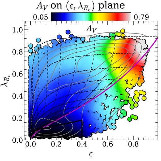
Distribution of AV (the attenuation of the spectrum at |$\lambda =5500\ \mathring{\rm A}$|, i.e. V band) on the |$(\epsilon , \lambda _{R_{\rm e}})$| plane (see Section 2.2 for definitions of these two parameters). The black polygon is defined by |$\lambda _{R_{\rm hsm}}=\epsilon /4+0.08$| and ϵ = 0.4, and encloses the region of slow-rotating ETGs (Cappellari 2016, equation 19). The magenta curve shows the edge-on view for axisymmetric galaxies following a relation between intrinsic shape and anisotropy β = 0.7ϵintr (Cappellari et al. 2007, fig. 9), with the black dotted lines showing its change with different inclinations (Δi = 10°). The black dashed lines show the theoretical distribution of galaxies versus inclinations, given different εintr values (Δεintr = 0.1). A kernel density estimation of the galaxy number density is indicated by the grey contours. This result comes from the ppxf fitting with the fsps stellar model.
We note here that the loess-smoothed values will be biased to a narrower range, and as a result, we shall not focus on the exact values of the properties, but focus on the overall trend of these quantities. The original values of all the population-related properties (including the dust attenuation parameters used here, the global stellar population properties used in Section 3, stellar population gradients used in Section 4, and SFH properties used in Section 5), the stellar population profiles, and the spatially resolved stellar population maps for all the |$\sim\!10\, 000$| galaxies are available from the website of MaNGA DynPop (https://manga-dynpop.github.io). The readers are referred to Table B1 for detailed explanations of the quantities. A brief comparison between this work and the existing stellar population catalogues for the MaNGA full sample, namely the pipe3d catalogue (Sánchez et al. 2022) and the firefly catalogue (Neumann et al. 2022) is given in Appendix A.
2.3.3 Global and spatially resolved stellar population properties
Spatially resolved spectra are typically binned to a higher S/N in order to get more accurate estimates of stellar population properties. In this work, we bin the spatially resolved spectra for each galaxy in two ways for different purposes:
We take the luminosity-weighted stellar population within the elliptical half-light isophote as the global stellar population properties of galaxies. To do so, we first bin, for each galaxy, all the spectra within the elliptical half-light isophote (the aperture size, ellipticity, and position angle of the elliptical half-light isophote can be obtained from Paper I) together and perform ppxf fitting on the derived spectra. In Fig. 4, we show the distributions of the S/Ns of the stacked spectra within half-light isophote and the number of stacked spaxels within this aperture. The S/N here is calculated as the ratio between the median values of flux and noise of the stacked spectra within the wavelength range from |$4730$| to |$4780\ \mathring{\rm A}$|, which does not include obvious emission and absorption lines. As can be seen, the elliptical half-light isophote typically contains a sufficiently large number of spaxels (with the median value being 387) and thus reaches a sufficiently high S/N (with the median value being S/N ∼ 342), with which the global stellar population properties can be accurately estimated.
To get the population property maps and further the population profiles/gradients, we first bin the spatially resolved spectra to S/N = 30 using the 2D adaptive spatial binning method (Cappellari & Copin 2003) with the VorBin9 software and perform ppxf to binned spectrum of each bin. We explain the calculation of population profiles/gradients in Section 4.
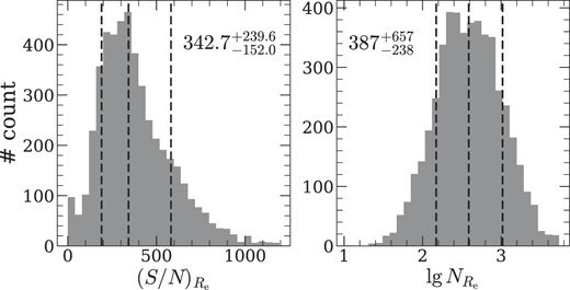
Distributions of signal-to-noise ratio (S/N) of stacked spectra within half-light isophotes (left panel) and the number of spaxels within half-light isophotes (right panel). In each panel, the three dashed lines represent 16 per cent, 50 per cent, and 84 per cent percentiles, respectively, from left to right, with the numbers indicating the corresponding values.
For both the stacked spectra within half-light isophote and the binned, spatially resolved spectra, we apply the ppxf fitting with the settings and assumptions described above to obtain the best-fitting template weights. With the best-fitting template weights from ppxf, luminosity age and metallicity of the spectrum can be calculated as
where x can be |$\lg \rm age$| or [Z/H]; wk and Lk are the best-fitting weight and SDSS r-band luminosity of the kth template, respectively. Stellar mass-to-light ratio is defined as
where M*, k is the stellar mass (including the mass of living stars and stellar remnants, but excluding the gas lost during stellar evolution) of kth templates. The summation goes over all the templates used in the fitting. The calculation of stellar mass-to-light ratio is automatically done by the mass_to_light routine of the ppxf software, which is independent of the dust attenuation effect. Throughout this paper, we only investigate luminosity-weighted stellar population properties, while the mass-weighted quantities will also be provided in the full catalogue (see Table B1).
In Fig. 5, we present the maps of stellar population properties (luminosity-weighted age, metallicity, and stellar mass-to-light ratio) of 30 examples (10 old galaxies, 10 galaxies with intermediate age, and 10 young galaxies). We note here that in principle the global stellar population properties can also be obtained by calculating the luminosity-weighted values of these properties within the half-light isophote on the spatially resolved population maps. Although there are discrepancies between the global stellar population properties within the half-light isophote derived from these two different ways, we confirm that our main results do not change with the definition of global stellar population properties.
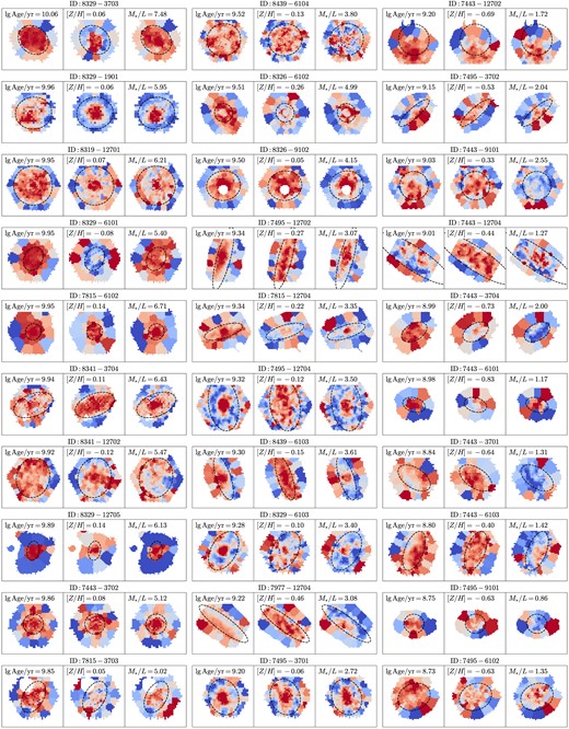
Examples of stellar population maps for 10 old galaxies (the left column), 10 galaxies of intermediate age (the middle column), and 10 star-forming galaxies (the right column). For each galaxy, we show their maps of luminosity-weighted age, metallicity, and stellar mass-to-light ratio from left to right, with their global stellar population property values shown in each panel. Redder colour corresponds to older age, higher metallicity, and larger stellar mass-to-light ratio. The black dashed ellipse in each panel represents the elliptical half-light isophote.
3 GLOBAL STELLAR POPULATION PROPERTIES
Stellar population properties have already been found to strongly correlate with structural and dynamical properties of galaxies, such as galaxy mass or velocity dispersion (e.g. McDermid et al. 2015; Scott et al. 2017; Li et al. 2018; see Cappellari 2016, section 4.3 for a review). In this section, we will present the correlations of galaxy (global) stellar population properties, including global age (|$\lg \, \mathrm{age}$|), metallicity ([Z/H]), and stellar mass-to-light ratio (M*/L), against structural and dynamical properties of galaxies for the MaNGA sample.
3.1 1D relation of stellar populations
In Fig. 6, we first present the 1D correlation between galaxy stellar population properties (i.e. age and metallicity) and the velocity dispersion for all the three SSP models (i.e. the fsps, the Vazdekis, and the galaxev models; see Section 2.3.1 for details of the three models). As shown in the figure, both age and metallicity show increasing trend with velocity dispersion for all the three SSP models, consistent with many previous studies (e.g. Kuntschner et al. 2010; Thomas et al. 2010; McDermid et al. 2015; Scott et al. 2017; Li et al. 2018). On the (σe, age) plane (top panels of Fig. 6), galaxies show clear bimodal distribution for all the three SSP models, classifying the galaxies into the well-known ‘red sequence’ (old and massive), ‘blue cloud’ (young and low-mass), and ‘green valley’ (intermediate age and intermediate mass) groups (e.g. Schawinski et al. 2014). It is present in all the three SSP models that the red sequence galaxies have relatively shallower σe–age relation, while blue cloud galaxies have a steeper one. This is consistent with the findings in Li et al. (2018), in which ETGs are seen to have smaller slope of the relation between velocity dispersion and galaxy age than spiral galaxies (see fig. 5 therein). All these confirm the robustness of our SPS results.
![Top panel: The distribution of global metallicity [Z/H] on the (σe, age) plane for the fsps, Vazdekis, and galaxev models from left to right. Bottom panel: The distribution of age $\lg \, \mathrm{age}$ on the (σe, [Z/H]) plane for the three stellar libraries. In each panel, a kernel density estimation of the galaxy number density is indicated by the grey contours.](https://oup.silverchair-cdn.com/oup/backfile/Content_public/Journal/mnras/526/1/10.1093_mnras_stad2732/1/m_stad2732fig6.jpeg?Expires=1749259914&Signature=4W5a8QI0uFmxRNCEi3uoIavNIfbgUIsAhLa7tW4lfBbQe4HkpINVzhqdfXnH1U59VQIuyQjw9qVOzo38yp-XKU8GdJnbD3LMVWeYGrxmVQClTx8oq3oOrPwAHi-zUaW0yv96neZani8ouP48-k2G15Wc-xCT5jOOUjyOk~j784meU0GZVPtqQ0oBMMr9xiZDY910IatWb~Qtu0B2O2bkyTqAXiuPqgy4~9QvpqN2Dg3R4BLiMuCh8pdGACktCZrRZI9E5T9ARQr8Sviq4Z6Wny2lQyjLxOHm4KlAbOdyhp4n6lnuhfvMA2aBQ7jzgopkBBvv-ctS7OuxUT0p7zcKBA__&Key-Pair-Id=APKAIE5G5CRDK6RD3PGA)
Top panel: The distribution of global metallicity [Z/H] on the (σe, age) plane for the fsps, Vazdekis, and galaxev models from left to right. Bottom panel: The distribution of age |$\lg \, \mathrm{age}$| on the (σe, [Z/H]) plane for the three stellar libraries. In each panel, a kernel density estimation of the galaxy number density is indicated by the grey contours.
Importantly, we find that metallicity shows obvious variation on the (σe, age) plane but it is not only driven by σe. At fixed σe, metallicity still increases with increasing age, especially for galaxies with |$\lg \, (\sigma _{\rm e}/\mathrm{km\, s^{-1}}) \lesssim 2.3$|. This strong decrease in metallicity with decreasing ages at fixed σe was also seen in a study at redshift z ≈ 0.8 by Cappellari (2020, fig. 6), which included both photometry and spectroscopy. The generality of this result, with completely different data and samples, confirms its robustness. The fsps and Vazdekis models show similar patterns of metallicity on the (σe, age) plane, with the fsps model showing more galaxies with younger age than the Vazdekis model. This is because that the age of the youngest stellar template in fsps is |$\lg \, \mathrm{age/yr}=6$|, significantly younger than that of the Vazdekis model (with the youngest age being |$\lg \, \mathrm{age/yr}=7.8$|). Besides, the Vazdekis model seems to provide too low metallicities due to the age–metallicity degeneracy (Worthey 1994): The fit tries to compensate for the lack of sufficiently young models by lowering the metallicity, which produces, to first order, a similar effect as lowering the age. The galaxev model, however, seems to be problematic and does not show similar metallicity pattern on the (σe, age) plane as the fsps and Vazdekis models do: Galaxies with intermediate age (|$\lg \, \mathrm{age/yr}\sim 9.5$|) with galaxev model appear to have the highest metallicity, while for the fsps and Vazdekis models, galaxies in the red sequence have the highest metallicity. This inconsistency is also seen in the bottom panels of Fig. 6, where we show the correlation between [Z/H] and |$\lg \, \sigma _{\rm e}$|, colour-coded by galaxy age. As can be seen, the fsps and Vazdekis models show similar age distribution on the (σe, [Z/H]) plane, with the Vazdekis model having more galaxies with lower metallicity, due to the lower metallicity boundary of the Vazdekis model (see Fig. 1). Besides, galaxy age show stronger correlation with metallicity than with σe as we can see that the age varies roughly along the direction of metallicity on the (σe, [Z/H]) plane. The galaxev model again shows difference with the fsps and Vazdekis models with metallicity being more strongly correlated with σe. The reason for the significantly different behaviour of the galaxev model would require further studies, but highlights the importance on not relying on a single set of modelling assumptions. Considering the problematic results of the galaxev model and the lack of youngest templates of the Vazdekis model, we take the fsps model as our default stellar library in the following sections. We note here that to fully understand the main driving factor of the stellar population variations as shown in Fig. 6, as well as the difference between the stellar libraries, a principal component analysis or a partial correlation analysis may be helpful, which is, however, beyond the scope of this paper. We encourage the interested readers to perform those analyses if necessary.
In Fig. 7, we present the distribution of total density slope of galaxies (see Section 2.2 for definition) on both the (σe, age) and the (σe, [Z/H]) planes. As can be seen, despite some subtle discrepancies, the total density slope shows an overall similar distribution as galaxy age (metallicity) on the two planes: Galaxies with higher σe, older age, and higher metallicity typically have larger total density slopes (i.e. steeper total mass profiles). The similar pattern on the two planes indicates a strong correlation between galaxy mass density slopes and stellar population properties, consistent with Cappellari (2016, fig. 22), where the total density slope of galaxies shows similar trend as stellar population properties on the mass–size plane. Interestingly, the total density slope is still seen to vary with age and metallicity at fixed σe, indicating that the correlation between stellar population and density slope is not solely driven by σe, consistent with the findings in Lu et al. (2020).
![Distribution of the dynamically determined total density slope on (σe, age; top panel) and (σe, [Z/H]; bottom panel) planes. Age and metallicity used here are derived with fsps models (see Section 2.3.1 for details of stellar models). In each panel, a kernel density estimation of the galaxy number density is indicated by the grey contours.](https://oup.silverchair-cdn.com/oup/backfile/Content_public/Journal/mnras/526/1/10.1093_mnras_stad2732/1/m_stad2732fig7.jpeg?Expires=1749259914&Signature=a3qXevRYFcIAAhFfExZrd7T2Cm272DW3GapKhEJ5ndc3f3IiNdZyInxqDfUZw0skSZv9Uz3nVsPKbX5-RaZQRrPX1mFk7gHQUQWylprXPNGhHMBW~R0XEsGuiuf3R4oEiGjPL0w4R5O1lgcoDe5757RjXoybQqbGqIGcZI-FiMu-l5csLtjcn4JL~KwWahwFCWk8zIKJs551psRrZ8AGgUQQvNac2DDkM0q753d2JFJzTQYM0ARk2IYbqjOEFz2VR3I3hDdsm91koO-Z0~Ac8wS~Yi58xi2bfSz5q0dqyQQ0FZHzr1uF7a4fuNinTLtY0eGag8PBDM7Y5xYtrvebTQ__&Key-Pair-Id=APKAIE5G5CRDK6RD3PGA)
Distribution of the dynamically determined total density slope on (σe, age; top panel) and (σe, [Z/H]; bottom panel) planes. Age and metallicity used here are derived with fsps models (see Section 2.3.1 for details of stellar models). In each panel, a kernel density estimation of the galaxy number density is indicated by the grey contours.
3.2 Stellar population on 2D planes
Apart from the 1D correlation between galaxy stellar population properties and galaxy velocity dispersion, we also show the distributions of stellar population properties on 2D dynamical/structural phase spaces.
In Fig. 8, we show the distributions of galaxy age, metallicity, and stellar mass-to-light ratio on the mass–size plane, |$(M_{\rm JAM},R_{\rm e}^{\rm maj})$| (see Section 2.2 for definitions of the two parameters). As shown in the figure, age, metallicity, and stellar mass-to-light ratio of galaxies all show systematic variations on the mass–size plane, ‘roughly’ along the direction of the virial estimate of the velocity dispersion σe, which accurately follows lines of |$R_{\rm e}^{\rm maj}\propto M_{\rm JAM}$| (Cappellari et al. 2013a). This is consistent with the positive correlation between stellar population properties and σe seen from Fig. 6.
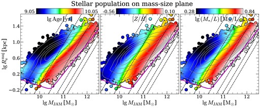
Distributions of age (left panel), metallicity (right panel), and stellar mass-to-light ratio (right panel) on the mass–size plane (|$\lg \, R_{\rm e}^{\rm maj}$| versus |$\lg \, M_{\rm JAM}$|; see Section 2.2 for definitions of the two parameters). In each panel, the black dashed lines indicate the lines of constant σe: 50, 100, 200, 300, 400, and 500 |$\mathrm{km\, s^{-1}}$|. The magenta curve is the zone of exclusion defined in Cappellari et al. (2013b). The galaxy number density is indicated by the grey contours.
In previous studies, the stellar velocity dispersion σ was found to be a better predictor of the galaxies M/L, which traces their stellar population, than stellar mass (Cappellari et al. 2006). Later, it was found to better predict galaxy colours (Franx et al. 2008) and stellar population from single fibres (Graves, Faber & Schiavon 2009). These early results were significantly strengthened by numerous studies using dynamical masses from integral field spectroscopy (IFS), all confirming that stellar population is better predicted by σ than M*. This was pointed out with ATLAS3D (McDermid et al. 2015; Cappellari 2016), SAMI (Scott et al. 2017; Barone et al. 2018, 2020), and MaNGA (Li et al. 2018), and even at significant redshift z ≈ 0.8 (Cappellari 2023).
Here we confirm again the general result, but we also find that the variation of stellar population properties is not strictly parallel with the constant-σe lines. At fixed σe, more massive galaxies appear to be slightly younger, more metal-poor, and have lower stellar mass-to-light ratio than the less massive galaxies. This is consistent with the findings of Lu et al. (2020), where the correlations between stellar population properties and other dynamical properties (i.e. the slope of galaxy velocity dispersion) at fixed σe are firmly observed. It means that mass density gradients (indicated by the velocity dispersion gradients) contain information of the stellar population which is not fully accounted for by σe. In addition, metallicity appear to have a better parallel correlation between constant-metallicity lines and constant-σe lines than age, also consistent with the smaller scatter of σe–[Z/H] relation than that of the σe–age relation in Fig. 6. It is worth pointing out, however, that the detailed location of galaxies on the mass–size diagram depends on how these quantities are measured, and one should be careful with interpreting subtle differences.
In Fig. 9, we show the distribution of stellar population properties on the |$(\epsilon ,\lambda _{R_{\rm e}})$| plane. As can be seen, slow-rotating galaxies (within the region of black lines) tend to be the oldest among all the galaxies and galaxy age show obvious decreasing trend with increasing |$\lambda _{R_{\rm e}}$| (i.e. become younger), consistent with van de Sande et al. (2018), in which the age distribution of 843 galaxies from the SAMI Galaxy Survey on the (ϵ, (V/σ)e) plane is studied.10 That is because rotation-dominated galaxies are more likely to be disc galaxies on the star-formation main sequence, as shown by Wang et al. (2020, fig. 2) for MaNGA galaxies (see also Fischer, Domínguez Sánchez & Bernardi 2019, fig. 27).

We also investigate the distributions of stellar metallicity and M*/L of galaxies on the |$(\epsilon ,\lambda _{R_{\rm e}})$| plane (the middle and right panels of Fig. 9), where we also see their systematic variations on the plane, which has never been seen before. We find that faster rotating galaxies tend to be more metal-poor and have lower M*/L. This is consistent with the trends we see on the |$(M_{\rm JAM},R_{\rm e}^{\rm maj})$| plane in Fig. 8, given that fast-rotating galaxies are those with smaller bulges and lower σe. To first order, the contours of constant ages or metallicity or M*/L follow the lines at which the galaxies of given flattening project for different inclination (the black dashed curves). This makes sense as one does not expect inclination to change the properties of the stellar population. However, the diagram also reveals some significant variations along the lines of constant intrinsic flattening. This is likely an effect due to dust and field coverage: For an edge-on view of galaxies, the observed population is dominated by the disc, which is typically more star-forming and thus is younger, more metal-poor, and has lower M*/L. The effect of inclination on the stellar population is generally ignored, because it is difficult to correct for it, but we show here how one can reveal its importance with the |$(\lambda _{R_{\rm e}},\epsilon)$| diagram.
4 POPULATION PROPERTY GRADIENTS
Apart from the scaling relation of global stellar population properties, we also study the scaling relations for stellar population gradients in this section. As mentioned in Section 2.3, the population profiles and gradients are derived from the spatially resolved stellar population maps, which are first Voronoi binned to S/N ∼ 30 before ppxf fitting. Pixels that are associated to the same Voronoi bin share the same age, metallicity, and stellar mass-to-light ratio. To calculate the stellar population profiles and gradients, we first divide the galaxies into different elliptical annuli with the radial step of each annulus being |$0.25R_{\rm e}^{\rm maj}$| along the major axis. The position angle and ellipticity of each annulus are set to be the same as the elliptical half-light isophote of the galaxy. For each annulus, we take the average luminosity-weighted stellar population properties as the value at this radius and then perform a linear fit to the radius–population relation. For age and stellar mass-to-light ratio, we take their values in logarithmic space into account (i.e. we fit the |$\lg \, \mathrm{age}-R/R_{\rm e}$| and |$\lg \, M_{\ast }/L-R/R_{\rm e}$| relations), while for metallicity, we fit the [Z/H]–R/Re correlation. We note here that due to the different observation ranges for different galaxies in MaNGA, the elliptical annuli are divided out the |$2R_{\rm e}^{\rm maj}$| along the major axis if applicable, while the stellar population gradients are only calculated within the elliptical half-light isophotes. For simplicity, we adopt the expression of ‘stellar population property at nRe’, instead of ‘stellar population within the elliptical annulus with semimajor axis being |$nR_{\rm e}^{\rm maj}$|’.
To better demonstrate this process, we present Fig. 10, where we show 12 examples of stellar population profile/gradient calculation, among which four galaxies have strong increasing age profiles within half-light isophote (i.e. significantly positive age gradient), four have nearly flat age profiles within half-light isophote (i.e. age gradient close to 0), and four have strong decreasing age profiles within half-light isophote (i.e. significantly negative age gradient). The thin grey dashed ellipses in each map are the boundaries of the radial bins and the thick black dashed ellipse is the elliptical half-light isophote, within which the stellar population gradients are calculated.
![Examples of stellar population profiles for four galaxies with significant positive age gradient (γage > 0.5, i.e. increasing age profile within half-light isophote; the left column), four with age gradient close to 0 (|γage| < 0.05, i.e. flat age profile within half-light isophote; the middle column), and four with significant negative age gradient (γage < −0.5, i.e. decreasing age profile within half-light isophote; the right column). For each galaxy, we show their age, metallicity, and stellar mass-to-light ratio maps (from left to right) in the top of each sub-figure, with thin dashed grey ellipses indicating the elliptical annuli within which the stellar population profiles are calculated, and the thick dashed black ellipse indicating the elliptical half-light isophote, within which the population gradients are calculated (see Section 4 for details). In the bottom panel of each sub-figure, the age, metallicity, and stellar mass-to-light ratio profiles are shown with blue, red, and green curves, respectively. Before plotting, the three profiles are shifted to have the same value in the innermost bin (0 < R < 0.25Re), so that the three profiles of different magnitudes can be plotted together. X in Y-axis of the panel can be $\lg \, \mathrm{age}$, [Z/H], and $\lg \, M_{\ast }/L$. The black dashed lines in the bottom panel of each sub-figure indicate the boundaries of each radial bin. The grey-shaded region indicates r < Re, within which the gradients of stellar population properties are calculated by performing a linear fitting to the profiles. Galaxy ID and the gradients of age, metallicity, and stellar mass-to-light ratio of each galaxy are shown on the top of each sub-figure.](https://oup.silverchair-cdn.com/oup/backfile/Content_public/Journal/mnras/526/1/10.1093_mnras_stad2732/1/m_stad2732fig10.jpeg?Expires=1749259914&Signature=Ard0qvcWJYxoD~zAJg3znqXwJtHkgJceDcIy~TpONJtA7e4OxYTi5jXWz17ANK~SyIrLd~wJgvKdVHbqm~l9c86bYmw0ThTNN48TwkM5-j9tVCNkOedKok4z-9LKuLsOF3faspOP6oXNHHsSOr7F8eootXxKPs4vPa65GNkDn4CNff6ATx2FpuUD6QAIYcxD8giVVJr0E-7BXqgqiQqPyPjdFlwHXbASS9CvP8p4wQEagg0MbXMLm1crNZuMpz73YlCaPl6d5GQQtJo1tC2LmB9Bvjk11Q9WsK2xYBNHxd2ZOprD0Tw~GbKox9ERWLJuXDWB4Y4E26VErplyRK25SQ__&Key-Pair-Id=APKAIE5G5CRDK6RD3PGA)
Examples of stellar population profiles for four galaxies with significant positive age gradient (γage > 0.5, i.e. increasing age profile within half-light isophote; the left column), four with age gradient close to 0 (|γage| < 0.05, i.e. flat age profile within half-light isophote; the middle column), and four with significant negative age gradient (γage < −0.5, i.e. decreasing age profile within half-light isophote; the right column). For each galaxy, we show their age, metallicity, and stellar mass-to-light ratio maps (from left to right) in the top of each sub-figure, with thin dashed grey ellipses indicating the elliptical annuli within which the stellar population profiles are calculated, and the thick dashed black ellipse indicating the elliptical half-light isophote, within which the population gradients are calculated (see Section 4 for details). In the bottom panel of each sub-figure, the age, metallicity, and stellar mass-to-light ratio profiles are shown with blue, red, and green curves, respectively. Before plotting, the three profiles are shifted to have the same value in the innermost bin (0 < R < 0.25Re), so that the three profiles of different magnitudes can be plotted together. X in Y-axis of the panel can be |$\lg \, \mathrm{age}$|, [Z/H], and |$\lg \, M_{\ast }/L$|. The black dashed lines in the bottom panel of each sub-figure indicate the boundaries of each radial bin. The grey-shaded region indicates r < Re, within which the gradients of stellar population properties are calculated by performing a linear fitting to the profiles. Galaxy ID and the gradients of age, metallicity, and stellar mass-to-light ratio of each galaxy are shown on the top of each sub-figure.
Interestingly, galaxies can have distinct profiles of different stellar population properties. For example, Galaxy 8459−1902 and Galaxy 8249−3703 (the middle two galaxies in the left column of Fig. 10) have significantly increasing age profiles from the galaxy centre towards the outskirts of the galaxies, while their metallicity profiles appear to be flat or even mildly decreasing. On the contrary, Galaxy 7443−12704 and Galaxy 7443−3701 (the first and third galaxies in the middle column of Fig. 10) have flat age profiles, but show significantly decreasing metallicity profiles from inner part to the outer part of the galaxies. In addition, the steepness of the stellar population profiles can change dramatically at different radii. For example, the luminosity-weighted age of Galaxy 7443−12703 (the first galaxy in the left column of Fig. 10) increases rapidly at small radii, but is nearly constant at R > Re. Galaxy 7443−6102 (the second galaxy in the middle column of Fig. 10) has an even more complicated age profile. This results in the fact that the stellar population gradients can be sensitive to the radial range they are estimated. Thus, the readers should be careful when comparing the results from different studies.
In Fig. 11, we present the radial profiles of age, metallicity, and stellar mass-to-light ratio for galaxies in different mass bins (|$\lg \, M_{\rm JAM}\ \lt\ 10.5$|, |$10.5\ \lt\ \lg \, M_{\rm JAM}\ \lt\ 11.5$|, and |$\lg \, M_{\rm JAM}\ \gt\ 11.5$|). As shown in the figure, galaxies with the lowest mass (|$\lg \, M_{\rm JAM}\ \lt\ 10.5$|) tend to have the youngest centre and a nearly flat age profile. It means that the galaxies with the lowest mass have active/recent star formation at all radii. The intermediate-mass galaxies (|$10.5\ \lt\ \lg \, M_{\rm JAM}\ \lt\ 11.5$|) appear to have a gradually decreasing age profile from galaxy centre to the outskirts. Interestingly, the most massive galaxies (|$\lg \, M_{\rm JAM}\ \gt\ 11.5$|) appear to have the oldest centre with the age profile being nearly flat within R ≲ Re, while show obviously decreasing age profiles towards larger radii at R ≳ Re with a large scatter. This again raises the importance of clarifying the radial range of gradient calculation. For metallicity, nearly all the galaxies in different mass bins show similar, decreasing metallicity profiles from the central region to the outer part of the galaxies, with the most massive galaxies (|$\lg \, M_{\rm JAM}\ \gt\ 11.5$|) having the highest metallicity at all radii. This is consistent with the findings of previous studies (e.g. Kuntschner et al. 2010; Goddard et al. 2017; Zheng et al. 2017; Li et al. 2018; Santucci et al. 2020), where galaxies are found more likely to have negative metallicity gradients (higher metallicity at galaxy centre). Besides, galaxies with the lowest mass have a mildly increasing M*/L profile, with the outer part of the galaxies having slightly higher M*/L. It means that on average, star formation is slightly more active at the outskirts of these galaxies. The intermediate-mass galaxies again show a gradually decreasing M*/L profile and the most massive galaxies again have gradually decreasing M*/L profile at small radii (R ≲ 1.5Re), which becomes steeper at larger radii (R ≳ 1.5Re) with large scatters. This result shows remarkable agreement with the study of Ge et al. (2021, fig. 4), where M*/L profile is also seen to be mass-dependent, and the steepness of M*/L profile varies with radius for galaxies in the most massive bin, confirming the robustness of our work.
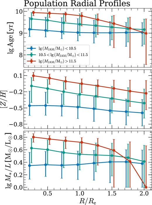
Radial profiles of age (top panel), metallicity (middle panel), and stellar mass-to-light ratio (bottom panel) of galaxies. In each panel, the median values of population radial profiles for galaxies with different masses are indicated by curves of different colours, with the error bars indicating the range from the 16th to the 84th percentiles (±1σ).
The young and low-M*/L outer region of massive galaxies and their large scatters at large radii (R ∼ 2Re) indicate that galaxies in this mass bin (i.e. |$\lg \, M_{\rm JAM}\ \gt\ 11.5$|) does not only consist of totally quenched galaxies but also contains massive disc galaxies. These disc galaxies typically have large, old, and quenched bulges at the galaxy centre, and gas-rich discs at the outskirts, which are still actively forming stars, making the outer part younger and to have lower stellar mass-to-light ratio (e.g. Lu et al. 2022a in simulations and Zhang et al. 2019 in observations).
This interpretation can be confirmed by Fig. 12, where we show the distributions of the gradients of age, metallicity, and stellar mass-to-light ratio (γage, γ[Z/H], and |$\gamma _{M_{\ast }/L}$|) on the mass–size plane. Unlike global stellar population properties (see Fig. 8), stellar population gradients show more complicated distributions on the mass–size plane. At the low-mass end (|$\lg \, M_{\rm JAM}\sim 9.6{-}9.8$|), galaxies with smaller sizes are more likely to have positive γage (younger centres and older outer parts), compared with those with the same mass but larger sizes. This is consistent with Lu et al. (2021), where part of low-mass disc galaxies have experienced more retrograde (with respect to their stellar spin) mergers and thus have counter-rotating gas discs and a high fraction of counter-rotating stars (with respect to the bulk of stellar rotation), making the galaxies to have smaller sizes and more centrally concentrated star formation, i.e. younger centre than outer part. Besides, galaxies with (|$\lg \, M_{\rm JAM}\sim 11{-}12$|) and |$\lg \, R_{\rm e}^{\rm maj}\gtrsim 1.2$| have the lowest γage (the steepest decreasing age profile from centre to the outskirts), consistent with the cartoon by Cappellari (2016, fig. 23), in which we can see that galaxies in this region are mainly massive disc galaxies with large, old, and quenched bulges at galaxy centre and star-forming discs at the outskirts of the galaxies. According to Cappellari (2016, fig. 23), massive galaxies contain both quenched elliptical galaxies, as well as the massive disc galaxies, consistent with our guess for the origin of the young outskirts and large scatters in age and stellar mass-to-light ratio of massive galaxies (|$\lg \, M_{\rm JAM}\ \gt\ 11.5$|) in Fig. 11. The gradients of metallicity and stellar mass-to-light ratio show similar distributions as the age gradient on the mass–size plane, with a subtle difference in metallicity gradient, where the galaxies with the flattest metallicity profiles locate in the region with intermediate mass and intermediate size (|$\lg \, R_{\rm e}^{\rm maj}\sim 0.6{-}1$| and |$\lg \, M_{\rm JAM}\sim 10{-}11$|). All the detailed features of the variation of galaxy gradients in this diagram agree remarkably well with the independent study by Li et al. (2018, fig.7), confirming the robustness of the trends.
![Distribution of age gradient (γage; left panel), metallicity gradient (γ[Z/H]; middle panel), and stellar mass-to-light gradient ($\gamma _{M_{\ast }/L}$; right panel) on the mass–size plane ($\lg \, R_{\rm e}^{\rm maj}$ versus $\lg \, M_{\rm JAM}$, see Section 2.2 for definitions of the two parameters). The symbols are the same as Fig. 8.](https://oup.silverchair-cdn.com/oup/backfile/Content_public/Journal/mnras/526/1/10.1093_mnras_stad2732/1/m_stad2732fig12.jpeg?Expires=1749259914&Signature=kZDfM1rzjN~EnoVhmjUavKe3J8G7mcCMR0OI8WWwnbNYphRBqQBXf6ZlwbBajTjwn0iVGHfX6PJ4kOu3kvqaT4ZEZPwp4Rp2D7n8FYL~7LZqsmzvpUopJfAPogLM72wTDMmD1Xlz~0JX2iH490YbOSRiw2O~uTAzcfF-VxNWHb4-kb5iyrwGlCFzpN~Q81L0y~dwaUDXRSr~F3JrW9bEassUBfCe1Or3a43h5ZEzNLS78xzBiLAG3iZL6U5yUgDimCK73MMmJYA0bya0b8DAiFmickHK35O9OS7Ljv8DseBsLjMqZto09p60IyKBC2RKoyzv4Lc6Qt38Xb61g5sYWQ__&Key-Pair-Id=APKAIE5G5CRDK6RD3PGA)
Distribution of age gradient (γage; left panel), metallicity gradient (γ[Z/H]; middle panel), and stellar mass-to-light gradient (|$\gamma _{M_{\ast }/L}$|; right panel) on the mass–size plane (|$\lg \, R_{\rm e}^{\rm maj}$| versus |$\lg \, M_{\rm JAM}$|, see Section 2.2 for definitions of the two parameters). The symbols are the same as Fig. 8.
The mass–size plane does not capture the main features of population gradients in galaxies. In fact, we find that there are major systematic trends in the gradients at fixed σe, namely at fixed location on the mass–size plane, as a function of galaxy age. In Fig. 13, we present the stellar population gradients on the (σe, age) plane, where |$\lg \, \mathrm{age}$| is the global luminosity-weighted age of galaxies (see Section 2.3.3 for the definition of global population properties). As can be seen, older galaxies with |$\lg \, \sigma _{\rm e}\gtrsim 2.0$| tend to have less-negative age gradients (closer to 0, indicating a flat age profile). This indicates that old galaxies are almost equally old at different radii. It may be caused by both a physical origin, where old and quenched galaxies have longer time to radially mix their stellar content, and a technical origin, where age differences are difficult to measure at the age older than |$8\, \rm Gyr$|. Interestingly, galaxies in the green valley, namely between the two peaks in the galaxy number density, appear to have the lowest γage (the most negative, indicating the steepest decreasing age profile from centre to the outer part of galaxies). This shows that that green valley galaxies are typically massive disc galaxies, which have quenched centres (bulges) and maintain star-forming discs at the outskirts. These results are consistent with Lah et al. (2023), which studied the differences of stellar population of bulges and discs in MaNGA and found that ETGs tend to have bulges and discs with similar age (i.e. flat age profiles), while LTGs have discs much younger than bulges (i.e. the steepest decreasing age profiles from galaxy centre to the outside).
![Distribution of age gradient (γage; left panel), metallicity gradient (γ[Z/H]; middle panel), and stellar mass-to-light gradient ($\gamma _{M_{\ast }/L}$; right panel) on the (σe, age) plane. The galaxy number density is indicated by the grey contours.](https://oup.silverchair-cdn.com/oup/backfile/Content_public/Journal/mnras/526/1/10.1093_mnras_stad2732/1/m_stad2732fig13.jpeg?Expires=1749259914&Signature=aCMGx-llkmN0xEoIkLhNY51~HUR-83ErN9hM~hYmQBIeGcFssEsgV5uTzKq7QgGzQ~1gztP8u2ZPTkvSFPSJgXqGJMTIVc9Dzin-PZCHTUQlAtNvw3LfzLJqWN6gAcSeZJ5rupuhcRAYHjFiskKcb692baTxJa-TFr8xH2w0oGbvj8mRFV9GfnLN6asz~Gd045oHvcxhDBF6FUHA73Us15m-GE0HKcuGcfPQV72H9l5gkwmcQF2EW~8cagaZuDphzBfGe7HLcH4YaL7TAVtvnR~HIaqznYfnhGkHO1mID1KfCxGYijjV81jhNlUbYcYScTV3k4E6jv7hcMPAtoqIPg__&Key-Pair-Id=APKAIE5G5CRDK6RD3PGA)
Distribution of age gradient (γage; left panel), metallicity gradient (γ[Z/H]; middle panel), and stellar mass-to-light gradient (|$\gamma _{M_{\ast }/L}$|; right panel) on the (σe, age) plane. The galaxy number density is indicated by the grey contours.
Metallicity gradient appears to have a stronger correlation with σe rather than with galaxy age, although strong variations exist at fixed σe and varying age. The most negative metallicity gradient is also seen for galaxies in the green valley (but have larger σe than those with the lowest age gradients), which may be because of the low-metallicity gas accretion of these galaxies diluting the metallicity. Given that the stellar mass-to-light ratio (M*/L) depends on both age and metallicity (e.g. fig. 2 of Ge et al. 2019), it makes sense that the distribution of gradient of M*/L on the (σe, age) plane is intermediate between the distributions of γage and γ[Z/H] on this plane.
In Fig. 14, we present the distributions of the three stellar population gradients on the |$(\epsilon ,\lambda _{R_{\rm e}})$| plane (see Section 2.2 for definitions of the two parameters). As can be seen, the most rotational galaxies have the lowest γage (the most negative, indicating the steepest decreasing age trend from centre to the outer part of galaxies), again consistent with the results seen from Figs 12 and 13. We note that galaxies with high |$\lambda _{R_{\rm e}}$| and large ϵ (i.e. edge-on), however, have flatter age profiles (less negative γage), compared with those with similar |$\lambda _{R_{\rm e}}$| but smaller ϵ (i.e. more face-on). That is because more disc component is observed for edge-on galaxies, making the averaged age younger at the centre (compared with the face-on view of the galaxy) and resulting in the flatter age profiles in these galaxies. In addition, the dust attenuation effect is also significantly stronger from the edge-on view of the galaxies, and its degeneracy with stellar age also potentially contributes to the flattening of stellar population gradients.
![Distribution of age gradient (γage; left panel), metallicity gradient (γ[Z/H]; middle panel), and stellar mass-to-light gradient ($\gamma _{M_{\ast }/L}$; right panel) on the $(\epsilon ,\lambda _{R_{\rm e}})$ plane (see Section 2.2 for definitions of the two parameters). The symbols are the same as Fig. 3.](https://oup.silverchair-cdn.com/oup/backfile/Content_public/Journal/mnras/526/1/10.1093_mnras_stad2732/1/m_stad2732fig14.jpeg?Expires=1749259914&Signature=LgbuezMa3OOWOmCWuPTxxXuixFlTvA4kZJktNDwOtmOTzjWMRLBxxapPkN3Ca7t4zvs3wXsaK4V1XiPUOfZDUZrSaZoYUpONrPHHDxGAxxth5TeVX65GAnlmCB3IkL4F7LmzK1xHBm~oYjM357vQebvwcx1-r~29ttjerD2irzQ84FcBD4vegs1izLImRGCV-pe7X-Zz-J23NoFHeAC6koz~-HAzebLDXakvrH0iPe-lHmbV~dM0guA1Nm4r3x7oUEQrF0G9K7PRurGBzAcoOOstS2htSOoLZJdHMKgaL5iU~rElOGOQCzFB0n94WOGCQ~zNnCsYtddL8OLPOAsSPQ__&Key-Pair-Id=APKAIE5G5CRDK6RD3PGA)
Distribution of age gradient (γage; left panel), metallicity gradient (γ[Z/H]; middle panel), and stellar mass-to-light gradient (|$\gamma _{M_{\ast }/L}$|; right panel) on the |$(\epsilon ,\lambda _{R_{\rm e}})$| plane (see Section 2.2 for definitions of the two parameters). The symbols are the same as Fig. 3.
The distribution of metallicity gradient on the |$(\epsilon ,\lambda _{R_{\rm e}})$| plane is more complicated. First, galaxies with the highest |$\lambda _{R_{\rm e}}$| (|$\lambda _{R_{\rm e}}\sim 0.8$|) and relatively low ϵ (ϵ ≲ 0.6) have the most negative γ[Z/H] (i.e. the steepest decreasing metallicity profiles from galaxy centre to the outskirts), same as the age gradient. Secondly, the most edge-on galaxies with intermediate/large |$\lambda _{R_{\rm e}}$| (|$0.3\lesssim \lambda _{R_{\rm e}}\lesssim 0.7$|) have the largest metallicity gradient (close to 0, i.e. flat metallicity profiles), different from the age gradients. Thirdly, the slow-rotating galaxies (within the region of black lines) appear to have intermediate γ[Z/H], indicating relatively obvious decreasing metallicity profiles of these galaxies. The distribution of gradient of stellar mass-to-light ratio again appears to be the combination of age gradient and metallicity gradient on the |$(\epsilon ,\lambda _{R_{\rm e}})$| plane, where galaxies with the highest |$\lambda _{R_{\rm e}}$| (|$\lambda _{R_{\rm e}}\sim 0.8$|) and relatively low ϵ (ϵ ≲ 0.6) have the steepest decreasing stellar mass-to-light ratio profiles and the most edge-on galaxies with intermediate |$\lambda _{R_{\rm e}}$| (|$0.1\lesssim \lambda _{R_{\rm e}}\lesssim 0.6$|) have the flattest stellar mass-to-light ratio profiles.
To further explore the interesting distribution of metallicity on the |$(\epsilon ,\lambda _{R_{\rm e}})$| plane, we present Fig. 15, where we show the distributions of galaxy mass and r-band luminosity (see Section 2.2 for the definitions of the two parameters) on this plane. As can be seen, galaxy mass and r-band luminosity show remarkably similar trends as metallicity gradient (see the middle panel of Fig. 14) on the |$(\epsilon ,\lambda _{R_{\rm e}})$| plane: The slow-rotating galaxies and the most rotation-supported galaxies appear to have the highest mass and luminosity (and the lowest metallicity gradients in the middle panel of Fig. 14), while the galaxies below the magenta curve (i.e. the ones being edge-on but having low |$\lambda _{R_{\rm e}}$|) appear to have the lowest mass and luminosity (and the flattest metallicity gradients in the middle panel of Fig. 14). Previously, many studies have pointed out the mass-dependence of metallicity gradient of galaxies (e.g. Carollo, Danziger & Buson 1993; Kuntschner et al. 2010; Sánchez-Blázquez et al. 2014; González Delgado et al. 2015; Ho et al. 2015; Goddard et al. 2017; Zheng et al. 2017; Santucci et al. 2020), but it is the first time to see their tight correlation on a 2D plane. We note that the mass distribution on the |$(\epsilon ,\lambda _{R_{\rm e}})$| plane is not consistent with that in Graham et al. (2018, fig. 9), especially for the most rotation-supported galaxies. The possible reason may be the different calculations of galaxy mass. The galaxy mass used in this work is totally based on dynamical modelling (see Section 2.2 and Paper I for details), while that used in Graham et al. (2018) is from the empirical correlation between dynamical mass and KS band magnitude, which is calibrated to ATLAS3D dynamical models for ETGs only (Cappellari 2013). The origin of the interesting distribution of metallicity gradient on the |$(\epsilon ,\lambda _{R_{\rm e}})$| plane and its tight correlation with galaxy mass (luminosity) may rely on the mass assembly histories of the galaxies, and is worth investigating with cosmological simulations. We plan to carry out this study in the following papers of this MaNGA DynPop series.

5 STAR-FORMATION HISTORY
SFH of galaxies is one of key things to analyse in studying the evolution of galaxies. In practice, one can obtain SFH of galaxies from their spectra using either parametric methods (by assuming the specific formula of SFH; e.g. Carnall et al. 2018; McLure et al. 2018; Zhou et al. 2020, 2021; see Carnall et al. 2019 for the comparison between different parametrizations), or non-parametric methods (by calculating the SFR from SSPs in each time bin; e.g. Cid Fernandes et al. 2005; McDermid et al. 2015; Cappellari 2017, 2023; Leja et al. 2019). In this work, we adopted the non-parametric method to study the SFH of MaNGA galaxies, using the ppxf software. ppxf combines the linear regularization method (e.g. Press et al. 2007), which enables the users to obtain a smoother SFH while keep the best-fitting spectrum nearly unchanged within the given uncertainty (see section 3.5 of Cappellari 2017 for details of regularization).
Before applying the regularization to the whole sample, we first investigate the effect of different regularization levels on the SFH with a random sub-sample of MaNGA by setting the regul keyword to be 0, 50, 100, and 300 (regul = 0 represents the non-regularized fitting which is used to derive stellar population properties and their gradients in the previous sections). In Fig. 16, we present several examples of ppxf fitting with different regul values. We note here that all the analyses of SFH in this work are based on the stacked spectrum within half-light isophotes of galaxies. As can be seen, with increasing regul value, the distribution of SSP template weight becomes more smoothed, while the fittings roughly maintain the star-formation epochs of the galaxies, although short star-forming episodes may be hidden. We confirm that fitting with different regul values provides nearly the same fitting goodness of the spectrum. In this work, we apply regul = 100 on the complete MaNGA sample to derive their SFHs and confirm that the choice of regul will not qualitatively change our results presented blow. We note here that due to the lack of near ultraviolet (NUV) and infrared (IR) spectrum in MaNGA survey, the SFH of individual galaxies may not be able to be well constrained. In particular, we are not very sensitive to small contributions of very recent star formation, which produce a blackbody peak in the UV due to the massive and hot stars and another blackbody distribution in the IR, due to the photons re-radiated by dust. However, by combining the large sample of MaNGA, we are still able to spot clues of the correlation between SFH and galaxy properties.
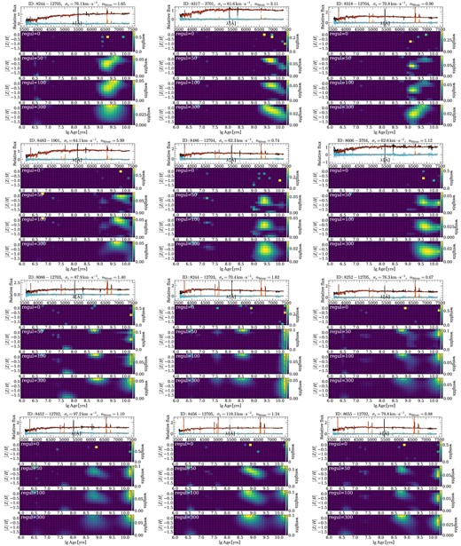
Examples of ppxf fitting results with different regul values. The top two rows are the galaxies whose SFH can be roughly approximated by a single star-formation burst. The bottom two rows show the galaxies with multiple star-formation bursts. For each galaxy, the fitted spectrum is the stacked spectrum within half-light isophote (see Section 2.3.3 for details). In each sub-figure, the observed and best-fitting spectra (without regularization, i.e. regul = 0) are shown in the top panel with black and red curves, respectively. The cyan diamonds denote the fitting residuals and the orange curve represent the gas-only best-fitting spectrum (see Section 2.3 and Fig. 2 for more details of spectrum fitting). Template weight distributions with different regul values (regul|$=0,\, 50,\, 100,\, 300$|) are shown in the panels from top to bottom. All these fittings are based on the fsps SSP model (see Section 2.3.1). Galaxy ID, velocity dispersion, and |$\rm S\acute{e}rsic$| index are shown in the top of each sub-figure. The |$\rm S\acute{e}rsic$| index used here is from the NSA catalogue (Blanton et al. 2011).
In Fig. 17, we present the correlation between SFHs and galaxy properties (see the caption of the figure). Here, we take the evolution of SFR and sSFR with cosmic time as the SFH of the galaxies. To calculate SFR at a given time, we first add up the initial stellar masses (set to be |$1\mathrm{{\rm M}_{\odot }}$| for each template) of all the templates with the same age (see Section 2.3.1 and Fig. 1 for age grids of the templates used in this work) and then re-bin the logarithmically spaced SFR on to a linear time axis (the time step is set to be 1Gyr), keeping the total newly formed stellar mass in each time step unchanged, similar to the practice of McDermid et al. (2015). sSFR is calculated as the instantaneous SFR divided by the existing stellar mass at that time. In each panel of Fig. 17, galaxies are first divided into 15 bins according to their properties (see the X-axes in Fig. 17), resulting in ∼400 galaxies in each bin. For each bin, we calculate the averaged SFR and sSFR at each time step. Below, we summarize the main conclusions shown in Fig. 17.
![SFH [represented by star-formation rate (SFR) in top panels and sSFR in bottom panels as a function of lookback time, tlb] versus galaxy properties: Velocity dispersion within Re ($\lg \, \sigma _{\rm e}$), total density slope (γtot), dark matter fraction within Re (fDM), stellar mass-to-light ratio from SPS non-regularized fitting (M*/L), and global metallicity ([Z/H]) from left to right. In each panel, galaxies are equally divided into 15 bins according to their properties (X-axis; about 400 galaxies in each bin). For galaxies in each bin, we re-bin their logarithmically spaced weights from ppxf ($\texttt {regul=100}$) onto a linear time axis with the time step being 1 Gyr. SFR and sSFR are then calculated as the averaged values of all the galaxies in each bin at each time step.](https://oup.silverchair-cdn.com/oup/backfile/Content_public/Journal/mnras/526/1/10.1093_mnras_stad2732/1/m_stad2732fig17.jpeg?Expires=1749259914&Signature=X0gm0CBAbc-5-c7IdsIFT~G-eixWQLl6UKZ2PssIz7aJze-x8S0pasV79p62bdq2x5k88cCwiSvhSz8jGg3tbpUs5LQGVXkZF2kjBPepSzHxukA7QV3VFeachquKo7ut3ygukjms~PvWfU1sh8BqNhKYEbGo4Z-vkzqTAsyWdWivhJvLQDrFUe1Lip8Bj0YPFdXQvBnh~SMEFc6a8gFMf35ILzgrv-ZWK9~kVlJihFkCLA-A4yXPHU4IjbhxnF-c5T5mrTc4DiX0sQqH9EDa8hb1N4bVtZlh77hwTEKHRzxK25vJg6Ge7Aww2NmvO6HNs~Bg0yTQAmU~BI1GTvNilg__&Key-Pair-Id=APKAIE5G5CRDK6RD3PGA)
SFH [represented by star-formation rate (SFR) in top panels and sSFR in bottom panels as a function of lookback time, tlb] versus galaxy properties: Velocity dispersion within Re (|$\lg \, \sigma _{\rm e}$|), total density slope (γtot), dark matter fraction within Re (fDM), stellar mass-to-light ratio from SPS non-regularized fitting (M*/L), and global metallicity ([Z/H]) from left to right. In each panel, galaxies are equally divided into 15 bins according to their properties (X-axis; about 400 galaxies in each bin). For galaxies in each bin, we re-bin their logarithmically spaced weights from ppxf (|$\texttt {regul=100}$|) onto a linear time axis with the time step being 1 Gyr. SFR and sSFR are then calculated as the averaged values of all the galaxies in each bin at each time step.
As show in the top panels of Fig. 17, SFR evolution tracks vary with all the five parameters. Specifically,
Galaxies with high |$\lg \, \sigma _{\rm e}$| (≳2.3) are found to have high SFR at high redshift and show obvious decreasing trend towards lower redshift. Below |$t_{\rm lb}\lesssim 2.4\, \mathrm{Gyr}$|, these galaxies become quenched and never form stars again, which presents a clear and sharp quenching boundary. The sharp boundary from star formation to quenching in this work is well consistent with the finding of Cappellari (2023), where a clear quenching boundary at |$\lg \sigma _{\rm e}\sim 2.3$| is also seen (see fig. 8 of Cappellari 2023). However, Cappellari (2023) also find a decreasing trend of the time when star formation of galaxies becomes the most active with the decreasing σe (i.e. galaxies with lower σe appear to show star-formation peak more recently), which is not seen in our results. Besides, in Cappellari (2023), galaxies with |$\lg \, \sigma _{\rm e}\gtrsim 2.3$| are found to get quenched at least 6.8 Gyr ago (the corresponding lookback time of the median redshift of LEGA-C galaxies, i.e. z ∼ 0.76), significantly earlier than |$2.4\, \mathrm{Gyr}$| in this work. To the contrary, galaxies with low |$\lg \, \sigma _{\rm e}$| (≲2.0) never have SFR as high as the galaxies with high σe, while maintain the active star formation across their whole history, consistent with Cappellari (2023). The results above are also consistent with the findings of previous studies (e.g. Heavens et al. 2004; Thomas et al. 2005; Panter et al. 2007; Guglielmo et al. 2015; McDermid et al. 2015), where massive galaxies are found to have decreasing star-formation activities with cosmic time and become quenched earlier (resulting in the earlier mass assembly), while the low-mass galaxies keep the star-forming status across the whole time range.
A similar sharp quenching boundary is also seen in the correlation between SFR evolution and the galaxy total density slope (γtot; see Section 2.2 for definition). Galaxies with the steepest total mass profile (γtot ≳ 2.1) show similar trend as the galaxies with |$\lg \, \sigma _{\rm e}\gtrsim 2.3$|, where they are also seen to have high SFR at high redshifts, while becomes quenched below |$t_{\rm lb}\lesssim 2.4\, \mathrm{Gyr}$|. Galaxies with flatter total density slope have continuous SFR until the present. These results indicate that galaxies with higher σe typically have steeper total density profiles, consistent with previous studies (e.g. Cappellari 2016, fig. 22c; Li et al. 2019, and Paper III of this series).
Galaxies with low dark matter fraction (fDM; see Section 2.2 for definition) appear to have similar SFR evolution trend as galaxies with high σe or steep total density slope (i.e. high γtot), where they have high SFR at the early universe and become quenched around 2.4 Gyr ago. However, fDM does not show clear quenching boundary as σe and γtot do, indicating that fDM is not tightly correlated with the other two parameters (i.e. σe and γtot; this will be studied in Paper III of this series).
Stellar mass-to-light ratio (M*/L) and metallicity of galaxies show similar correlation of SFR evolution history with σe, because they tightly correlate with σe (see Fig. 8; also see McDermid et al. 2015; Cappellari 2016; Scott et al. 2017; Li et al. 2018). A clear quenching boundary is seen at M*/L ≳ 5 and [Z/H] ≳ 0, respectively.
We note here that our result (i.e. SFR decreases with cosmic time) also disagrees with the findings of Madau & Dickinson (2014), where the cosmic star-formation density peaks at z ∼ 2 (see fig. 9 therein). It may be due to the lack of low-mass galaxies in our sample, which contributes to the star-formation activities at lower redshifts. Also, the lack of near-infrared (NIR)/UV constraints in our study may be another cause of the discrepancy. We will combine the NIR/UV constraints and the optical spectra to study the SFHs of MaNGA galaxies in a forthcoming paper.
The sSFR evolution tracks, however, show different correlation with galaxy properties, compared with SFR evolutions. We note here that when calculating SFR and sSFR, we assume the SFR between two neighbouring age grids (see Fig. 1 for age grid design of the fsps model) to be constant. Thus, at early times (where the time step between two neighbouring age grids is significantly larger than 1 Gyr), the ratio between the instantaneous SFR and the existing stellar mass (i.e. the instantaneous sSFR) is also a constant for all galaxies (see the bottom panels of Fig. 17). This feature is also seen in McDermid et al. (2015, fig. 16), where galaxies in different mass bins have the same sSFR at early times. Despite the calculation issue here, we are also able to see some interesting features of the correlation between galaxy sSFR evolution trend and galaxy properties. Galaxies show clear quenching boundary for all the five parameters (including fDM, which does not show clear quenching boundary in its correlation with SFR evolution tracks). However, the quenching regions are not as regular as those for SFR. Specifically,
Galaxies with |$\lg \, \sigma _{\rm e}\gtrsim 2.1$| (unlike |$\lg \, \sigma _{\rm e}\gtrsim 2.3$| for SFR) appear to be quenched at the present day, while galaxies with higher σe are found to quench their star formation slightly earlier (3.6 Gyr ago for galaxies with |$\lg \, \sigma _{\rm e}\sim 2.5$|, relative to 2.4 Gyr ago for galaxies with |$2.1\lesssim \lg \, \sigma _{\rm e}\lesssim 2.5$|). Interestingly, galaxies with low σe appear to have double peaks of sSFR, both at early times and the present.
Galaxies with γtot ≳ 2.0 and fDM ≲ 0.5 become quenched about 2.4 Gyr ago, while galaxies with flat total density slope and high dark matter fraction appear to have double-peak sSFR evolution tracks.
A clear quenching boundary is also seen at M*/L ∼ 4 and galaxies with high stellar mass-to-light ratio appear to be quenched earlier (6 Gyr ago for galaxies with M*/L ∼ 7.5, relative to 2.4 Gyr ago for those with M*/L ∼ 5). A double-peak sSFR evolution track for galaxies with low M*/L is also seen.
Unlike σe and M*/L, metallicity of galaxies has a more regular quenching region, where galaxies with [Z/H] ≳ −0.2 are quenched 2.4 Gyr ago.
With SFR evolution tracks of all the galaxies, we are also able to predict the mass assembly histories of the galaxies. In Fig. 18, we present the distribution of t50 and t90 on the mass–size plane, where t50 and t90 are the lookback times when galaxies reach 50 per cent and 90 per cent of their present-day stellar mass. As can be seen, both t50 and t90 show systematic variation on the mass–size plane, similar to global stellar population properties (see Fig. 8): Galaxies with large σe tend to have larger t50 and t90, indicating earlier mass assembly of these galaxies, consistent with previous studies (e.g. McDermid et al. 2015; Zhou et al. 2021; Lu et al. 2022b). Besides, the constant-t50 (or constant-t90) lines are also not strictly parallel with constant-σe lines, indicating that the SFH properties of galaxies are also not fully accounted for by σe, similar to global stellar population properties (see Fig. 8).
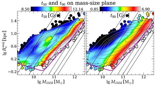
t50 and t90 on the mass–size plane (|$\lg \, R_{\rm e}^{\rm maj}$| versus |$\lg \, M_{\rm JAM}$|, see Section 2.2 for definitions of the two parameters), where t50 and t90 are the time when galaxies reach 50 per cent and 90 per cent of their present-day stellar mass, respectively. The symbols are the same as Fig. 8.
6 CONCLUSION
This work is the second paper of our MaNGA DynPop project, which aims to analyse the stellar population properties and SFH of the final MaNGA sample (SDSS data release 17; Abdurro’uf et al. 2022). In this paper, we make use of the SPS method to study the stellar population of the galaxies and use the non-parametric way to analyse their SFH. All these are done using the ppxf (Cappellari & Emsellem 2004; Cappellari 2017, 2023) software with the fsps stellar model. We summarize the main contents of this paper below:
We provide a catalogue which contains the global stellar population properties, the stellar population radial profiles, gradients, the spatially resolved stellar population maps, as well as the SFHs of |$\sim\!10\, 000$| MaNGA galaxies. The catalogue is available from the website of MaNGA DynPop (https://manga-dynpop.github.io). The explanations of the quantities of the catalogue are presented in Table B1.
With the derived global stellar population properties (i.e. age, metallicity, and stellar mass-to-light ratio), we revisit the scaling relation between stellar population properties and velocity dispersion of galaxies (Fig. 6), the distribution of total mass density slope on the (σe, age) and (σe, [Z/H]) planes (Fig. 7), and the distribution of stellar population on the mass–size plane (Fig. 8) and on the |$(\epsilon ,\lambda _{R_{\rm e}})$| plane (Fig. 9). We confirm that the positive correlation between global stellar population properties and velocity dispersion, the systematic variation of stellar population properties on the mass–size plane, as well as the variation of age on the |$(\epsilon ,\lambda _{R_{\rm e}})$| plane in previous studies (e.g. Cappellari et al. 2013b; McDermid et al. 2015; Cappellari 2016; Scott et al. 2017; Li et al. 2018; van de Sande et al. 2018) are all well recovered and also find some more interesting new results:
Variation of galaxy age and metallicity is not solely driven by velocity dispersion of galaxies, as we can see clear variation trend of age (metallicity) with metallicity (age) at fixed σe (Fig. 6). Total mass density slope show similar distributions on the (σe, age) and (σe, [Z/H]) planes as stellar population properties, indicating its tight correlation with stellar populations (Fig. 7).
Metallicity and stellar mass-to-light ratio are seen to have similar systematic variations on the |$(\epsilon ,\lambda _{R_{\rm e}})$| plane as galaxy age, which has not been reported before, with the less rotational galaxies (i.e. lower |$\lambda _{R_{\rm e}}$|) being older, more metal-rich, and having higher stellar mass-to-light ratio at fixed ϵ. The most edge-on galaxies have the youngest age, the lowest metallicity, and the lowest stellar mass-to-light ratio for the reason that more disc components (which are young, metal-poor, and have low stellar mass-to-light ratio) are observed for edge-on galaxies (Fig. 9).
We also study the stellar population profiles of galaxies with different mass. We find that the galaxies in the lowest mass bin tend to have flatter population profiles, while the ones in the highest mass bin have older centre with high M*/L and significantly young outskirts, with low M*/L (Fig. 11). This is because the highest mass bin contains not only the quenched elliptical galaxies, but also the massive disc galaxies with large quenched bulge at the centre and star-forming disc at the outer part. This is consistent with the findings in Figs 12 and 13, where the galaxies with the steepest stellar population profiles (i.e. the most negative population gradients) appear to be in the massive disc region (Fig. 12, see also fig. 23 of Cappellari 2016) or in the green valley (Fig. 13).
Systematic variations of stellar population slopes are also observed on the |$(\epsilon ,\lambda _{R_{\rm e}})$| plane. Galaxies that are rotational and have relatively low ϵ (≲ 0.6) have the lowest gradients of age and stellar mass-to-light ratio (i.e. the steepest decreasing age and stellar mass-to-light ratio profiles from centre to the outer part of galaxies). Galaxies with the flattest stellar population profiles locate in the region of largest ϵ (i.e. the most edge-on view of galaxies), because the more disc component observed from the edge-on view of galaxies contribute younger population to the galaxy centre, flattening the profiles (Fig. 14). Interestingly, metallicity gradient shows remarkably similar distribution as mass and luminosity of galaxies on the |$(\epsilon ,\lambda _{R_{\rm e}})$| plane, confirming the mass dependence of metallicity gradients (Figs 14 and 15).
Galaxies with different properties are found to have different SFHs. The galaxies with high, steep total density slope, low dark matter fraction, high stellar mass-to-light ratio, and high metallicity appear to have significantly higher SFR at early times, which decreases with cosmic time obviously, compared with other galaxies. Clear and regular quenching boundary are seen for the correlation between SFR evolution and galaxy properties (galaxies with |$\lg \, \sigma _{\rm e}\gtrsim 2.3$|, γtot ≳ 2.1, M*/L ≳ 5, or [Z/H] ≳ 0 are found to be quenched |$\sim\!2.4\rm\ Gyr$| ago). For sSFR evolution, however, the quenched regions are still seen but appear to be more complicated than that of SFR (Fig. 17). The lookback times when galaxies reach 50 per cent and 90 per cent of their present-day stellar mass (t50 and t90) are seen to have systematic variations on the mass–size plane, similar as stellar population properties (Fig. 18).
ACKNOWLEDGEMENTS
We thank the referee for the insightful comments which improved the paper. We also acknowledge Dr. Junqiang Ge, Dr. Shuang Zhou, and Dr. Niu Li for helpful discussions on the stellar population synthesis and Paul Tol for making his colour blind friendly colour schemes publicly available. This work is partly supported by the National Key Research and Development Program of China (No. 2018YFA0404501 to SM), by the National Natural Science Foundation of China (Grant No. 11821303, 11761131004, and 11761141012). This project is also partly supported by Tsinghua Initiative Scientific Research Program ID 2019Z07L02017. We also acknowledge the science research grants from the China Manned Space Project with No. CMS-CSST-2021-A11. KZ and RL acknowledge the support of National Natural Science Foundation of China (Nos. 11988101, 11773032, and 12022306), the support from the Ministry of Science and Technology of China (No. 2020SKA0110100), the science research grants from the China Manned Space Project (Nos. CMS-CSST-2021-B01 and CMS-CSST-2021-A01), CAS Project for Young Scientists in Basic Research (No. YSBR-062), and the support from K. C. Wong Education Foundation.
Funding for the Sloan Digital Sky Survey IV (SDSS-IV) has been provided by the Alfred P. Sloan Foundation, the U.S. Department of Energy Office of Science, and the Participating Institutions.
SDSS-IV acknowledges support and resources from the Center for High Performance Computing at the University of Utah. The SDSS website is www.sdss.org.
SDSS-IV is managed by the Astrophysical Research Consortium for the Participating Institutions of the SDSS Collaboration including the Brazilian Participation Group, the Carnegie Institution for Science, Carnegie Mellon University, Center for Astrophysics| Harvard & Smithsonian, the Chilean Participation Group, the French Participation Group, Instituto de Astrofísica de Canarias, The Johns Hopkins University, Kavli Institute for the Physics and Mathematics of the Universe (IPMU) University of Tokyo, the Korean Participation Group, Lawrence Berkeley National Laboratory, Leibniz Institut für Astrophysik Potsdam (AIP), Max-Planck-Institut für Astronomie (MPIA Heidelberg), Max-Planck-Institut für Astrophysik (MPA Garching), Max-Planck-Institut für Extraterrestrische Physik (MPE), National Astronomical Observatories of China, New Mexico State University, New York University, University of Notre Dame, Observatário Nacional/MCTI, The Ohio State University, Pennsylvania State University, Shanghai Astronomical Observatory, United Kingdom Participation Group, Universidad Nacional Autónoma de México, University of Arizona, University of Colorado Boulder, University of Oxford, University of Portsmouth, University of Utah, University of Virginia, University of Washington, University of Wisconsin, Vanderbilt University, and Yale University.
DATA AVAILABILITY
All the stellar population properties and star-formation history properties used in this work are publicly available on the website of MaNGA DynPop (https://manga-dynpop.github.io). The structural and dynamical properties can be obtained from Paper I, which are also publicly available from both the journal website and the website of MaNGA DynPop.
Footnotes
Version 6.3.3, available from https://pypi.org/project/jampy/.
Version 5.0.14, available from https://pypi.org/project/mgefit/.
Version 8.2.3, available from https://pypi.org/project/ppxf/. Also see Ge et al. (2018) for the comparison between the ppxf software and the starlight software (Cid Fernandes et al. 2005).
Available from https://github.com/cconroy20/fsps.
Available from http://www.bruzual.org/bc03/.
Available from http://miles.iac.es.
Version 2.1.2, available from https://pypi.org/project/loess/.
Version 3.1.5, available from https://pypi.org/project/vorbin/.
firefly also has a version based on the mastar stellar library (Yan et al. 2019).
References
APPENDIX A: COMPARISON WITH EXISTING CATALOGUES
In this section, we make comparisons with the existing stellar population catalogues of the full MaNGA sample, namely the pipe3d catalogue (Sánchez et al. 2022) and the firefly catalogue (Neumann et al. 2022). Both catalogues have provided a wealth of properties of stellar populations, emission lines, as well as the dust attenuation, which contribute to the legacy of the MaNGA project.
In Fig. A1, we present the comparisons of (global) luminosity-weighted age and metallicity, as well as their radial gradients between our work and the two catalogues. We note that both the pipe3d catalogue and the firefly catalogue provide the stellar population properties within a ring at effective radius as the global properties of the galaxies, while in our work, the average values within the elliptical half-light isophotes are used. Thus, to make a more accurate comparison, we also calculate the stellar population properties at effective radius by simply averaging the properties within the radial range of 0.75–1Re and 1–1.25Re (already provided in the catalogue of this paper under ‘Part 4: Stellar Population Radial Profiles’). When calculating the luminosity-weighted stellar populations, the pipe3d catalogue adopted the geometric means (i.e. |$\lt \lg \, x\gt $|, where x can be age and (Z/H)/(Z⊙/H⊙); same as this work), while the firefly catalogue adopted the arithmetic means (i.e. |$\lg \, \lt x\gt $|). Thus, when making comparison with the pipe3d catalogue, we keep our default setting (i.e. the geometric means) and when compared with the firefly catalogue, we re-calculate the global stellar population (at effective radius) and the corresponding stellar population gradients with the same arithmetic means as firefly for consistency. For the stellar population gradients, the two catalogues calculated them within different radial ranges (0.5–2Re for the pipe3d catalogue and 0–1.5Re for the firefly catalogue). To keep the consistency, we calculate the population gradients in the same radial ranges when comparing with the two catalogues (see Section 4 and Fig. 10 for the method of gradient calculation).
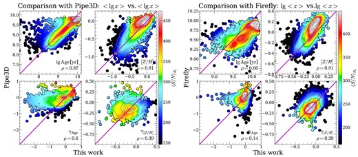
Comparisons between the stellar population properties of this work and those from the pipe3d (left sub-figure; Sánchez et al. 2022) and the firefly (right sub-figure; Neumann et al. 2022) catalogues. In both sub-figures, we present the comparisons of (i) luminosity-weighted age at effective radius (top-left panel), (ii) luminosity-weighted metallicity at effective radius (top-right panel), (iii) the slope of luminosity-weighted age profile (bottom-left panel; calculated within 0.5–2Re for pipe3d and 0–1.5Re for firefly), and (iv) the slope of luminosity-weighted metallicity profile (bottom-right panel; calculated within 0.5–2Re for pipe3d and 0–1.5Re for firefly). For the comparison with pipe3d catalogue (left sub-figure), we adopt the geometric means (i.e. |$\lt \lg \, x\gt $|, where x can be age and (Z/H)/(Z⊙/H⊙)) when calculating the luminosity-weighted values (which is also the default setting of this work), while we adopt the arithmetic means (i.e. |$\lg \, \lt x\gt $|) when comparing with the firefly catalogue (right sub-figure) for consistency. In each panel, the colours indicate the S/N of the stacked spectrum within the elliptical half-light isophotes and the magenta line indicates the y = x correlation. The Spearman rank-order correlation coefficient, ρ, is shown in the bottom right of each panel. The galaxy number density is indicated by the grey contours.
In the left sub-figure of Fig. A1, we show the comparison between our catalogue and the pipe3d catalogue. As can be seen, both global age and metallicity (measured at effective radius) in our work show good agreement with those from the pipe3d catalogue, with the Spearman rank-order correlation coefficient, ρ, being 0.87 and 0.81, respectively. Specifically, our age is slightly (|$\sim\!0.1 \rm \, dex$|) higher than pipe3d, while our metallicity is slightly lower. Our age gradient also shows consistency with the pipe3d catalogue (ρ = 0.6), while the galaxies with the most negative age gradient (the steepest decreasing age profiles from centre to the outer part of the galaxies) in our catalogue show flatter age profiles (i.e. less negative age gradient) in the pipe3d catalogue. The metallicity gradient, however, show weaker agreement between pipe3d (ρ = 0.39). Interestingly, we find that galaxies with higher S/Ns show stronger agreement between the two catalogues than those with low S/Ns.
For the comparison with the firefly catalogue, which is shown in the right sub-figure of Fig. A1, we find that the agreement of global age and metallicity (at effective radius; arithmetic means used) between the two catalogues is still seen, with the Spearman rank-order correlation coefficients being 0.66 for age and 0.81 for metallicity. Global age of firefly is systematically |$\sim\!0.3\, \rm dex$| lower than our result, while the global metallicity is systematically higher. Again, we can see that the galaxies which have the strongest disagreement between the two catalogues are typically those with low S/N. Wilkinson et al. (2017) pointed out the disagreement between the firefly software and the starlight software (Cid Fernandes et al. 2005), where the age of young galaxies in firefly is systematically older than that from starlight (see fig. 25 therein). Neumann et al. (2022) also pointed out the similar trend when comparing with the pipe3d catalogue (see fig. 13 therein). We emphasize here that these comparisons are not fair as the arithmetic means is used in firefly (i.e. |$\lg \, \lt x\gt $|), while the geometric means is used in starlight and pipe3d (i.e. |$\lt \lg \, x\gt $|). In Fig. A2, we compare our results with geometric means (i.e. |$\lt \lg \, x\gt $|) to those from firefly with arithmetic means (i.e. |$\lg \, \lt x\gt $|). We can see that we are also able to recover the similar trend as fig. 25 of Wilkinson et al. (2017) and fig. 13 of Neumann et al. (2022) with an independent software, ppxf. However, when we adopt the same arithmetic means (see the right sub-figure of Fig. A1), the firefly shows systematic lower age, rather than older age for young galaxies, as shown in Fig. A2 (also see fig. 25 of Wilkinson et al. 2017 and fig. 13 of Neumann et al. 2022).
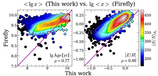
Unfair comparison of global age and metallicity (both are measured at effective radius) between our results and firefly. For our results, we adopt the geometric means (i.e. |$\lt \lg \, x\gt $|) to calculate the global stellar population properties, while firefly adopted the arithmetic means (i.e. |$\lg \, \lt x\gt $|). The symbols are the same as Fig. A1.
For the age and metallicity gradients, neither the age gradient, nor the metallicity gradient shows obvious agreement between our catalogue and the firefly catalogue. This may be due to the fact that the firefly catalogue is obtained from the ‘VOR10’ DAP output of MaNGA, which is Voronoi binned (Cappellari & Copin 2003) to S/N ∼ 10, while we bin our data to S/N ∼ 30. The low S/N may cause large noise at outer region of galaxies in estimating stellar population properties, which cannot be fixed by averaging. We also note here that the three catalogues (i.e. the pipe3d, the firefly, and the catalogue provided in this work) adopt totally different stellar libraries, which may also induce differences: The pipe3d catalogue adopted the mastar_slog library, which is based on the mastar MaNGA stellar library (Yan et al. 2019); the firefly catalogue adopted the m11-miles model templates from Maraston & Strömbäck (2011);11 and our results are based on the fsps model (see Section 2.3.1 for details). Considering the difference in the stellar libraries (and hence the boundaries of age and metallicity of the stellar templates), the fitting processes, the dust attenuation correction methods, and the definitions of effective radius, we actually do not expect all results to be consistent. We encourage the readers to make detailed comparisons when necessary.
APPENDIX B: DATA EXPLANATION
Data explanations of the stellar population analysis output (based on ppxf software with fsps stellar model; see Section 2.3 for details). The full catalogue of all the stellar population properties and SFH parameters used in this paper can be obtained from the website of MaNGA DynPop (https://manga-dynpop.github.io). The order of galaxies in this catalogue corresponds to their order in the JAM catalogue of Paper I.
| Parameters | Dimensions | Units | Descriptions |
|---|---|---|---|
| Part 1: General galaxy properties | |||
| plateIFU | (10 296,1) | The plate ID + IFU design ID (e.g. 7443–12 703; unique for each galaxy) | |
| mangaid | (10 296,1) | Unique MaNGA ID (e.g. 1–114 145) | |
| obj_ra | (10 296,1) | degree | Right ascension of the science object in J2000 |
| obj_dec | (10 296,1) | degree | Declination of the science object in J2000 |
| ebvgal | (10 296,1) | E(B − V) value from SDSS dust routine for this IFU | |
| z | (10 296,1) | Redshift of the galaxy | |
| Part 2: Global stellar population properties | |||
| SNR_Re | (10 296,1) | The S/N of the stacked spectrum within the elliptical half-light isophote, which is calculated as the ratio between the median values of flux and noise of the stacked spectra within the wavelength range from |$4730$| to |$4780\ \mathring{\rm A}$| | |
| Mstar_Re | (10 296,1) | |$\lg\ (\mathrm{{\rm M}_{\odot }})$| | Stellar mass enclosed within the elliptical half-light isophote, derived using ppxf with a Salpeter (1955) IMF |
| Lr_int_Re | (10 296,1) | |$\lg\ (\mathrm{L_{\odot }})$| | The intrinsic r-band luminosity within the elliptical half-light isophote, derived from the stacked intrinsic spectrum within the same aperture (see Section 2.3.2 for details) |
| Lr_obs_Re | (10 296,1) | |$\lg\ (\mathrm{L_{\odot }})$| | The observed r-band luminosity within the elliptical half-light isophote, derived from the stacked observed spectrum within the same aperture (see Section 2.3.2 for details) |
| LW_Age_Re | (10 296,1) | |$\lg\ (\mathrm{yr})$| | Global r-band luminosity-weighted age, calculated by performing ppxf fitting on the stacked spectrum within elliptical half-light isophote |
| LW_Metal_Re | (10 296,1) | Global r-band luminosity-weighted [Z/H] | |
| MW_Age_Re | (10 296,1) | |$\lg\ (\mathrm{yr})$| | Global mass-weighted age |
| MW_Metal_Re | (10 296,1) | Global mass-weighted [Z/H] | |
| ML_int_Re | (10 296,1) | |$\lg\ (\mathrm{{\rm M}_{\odot }/L_{\odot }})$| | Averaged intrinsic stellar mass-to-light ratio within the elliptical half-light isophote (calculated as the stellar mass enclosed within the elliptical half-light isophote and the r-band luminosity derived from the intrinsic spectrum within the same aperture; see Section 2.3.2 and Fig. 2 for definition of the intrinsic spectrum) |
| ML_obs_Re | (10 296,1) | |$\lg\ (\mathrm{{\rm M}_{\odot }/L_{\odot }})$| | Averaged observed stellar mass-to-light ratio within the elliptical half-light isophote (calculated as the stellar mass enclosed within the elliptical half-light isophote and the r-band luminosity derived from the observed spectrum within the same aperture) |
| Av_Re | (10 296,1) | Best-fitting dust attenuation at |$\lambda = 5500\ \mathring{\rm A}$| (V band; see Cappellari 2023, section 3.7 for details) | |
| delta_Re | (10 296,1) | Best-fitting UV slope of the spectrum (see Cappellari 2023, section 3.7 for details) | |
| Fred_tot_Re | (10 296,1) | r-band luminosity ratio between the observed spectrum and the intrinsic spectrum | |
| Fred_gal_Re | (10 296,1) | r-band luminosity ratio between the observed spectrum (with the MW dust attenuation corrected) and the intrinsic spectrum | |
| Part 3: Stellar population gradients | |||
| LW_Age_Slope | (10 296,1) | dex/Re | Gradient of r-band luminosity-weighted age within the elliptical half-light isophote (see Section 4 and Fig. 10 for details) |
| LW_Metal_Slope | (10 296,1) | dex/Re | Gradient of r-band luminosity-weighted [Z/H] within the elliptical half-light isophote |
| MW_Age_Slope | (10 296,1) | dex/Re | Gradient of mass-weighted age within the elliptical half-light isophote |
| MW_Metal_Slope | (10 296,1) | dex/Re | Gradient of mass-weighted [Z/H] within the elliptical half-light isophote |
| ML_int_Slope | (10 296,1) | dex/Re | Gradient of intrinsic r-band stellar mass-to-light ratio within the elliptical half-light isophote |
| ML_obs_Slope | (10 296,1) | dex/Re | Gradient of observed r-band stellar mass-to-light ratio within the elliptical half-light isophote |
| Part 4: Stellar population radial profiles | |||
| LW_Age_Profile | (10 296,8) | |$\lg\ (\mathrm{yr})$| | Radial profile of r-band luminosity-weighted age from 0 to 2Re with the radial step being 0.25Re (i.e. eight radial bins for each galaxy; see Section 4 and Fig. 10 for details) |
| LW_Metal_Profile | (10 296,8) | Radial profile of r-band luminosity-weighted [Z/H] | |
| MW_Age_Profile | (10 296,8) | |$\lg\ (\mathrm{yr})$| | Radial profile of mass-weighted age |
| MW_Metal_Profile | (10 296,8) | Radial profile of mass-weighted [Z/H] | |
| ML_int_Profile | (10 296,8) | |$\lg\ (\mathrm{{\rm M}_{\odot }/L_{\odot }})$| | Radial profile of intrinsic r-band stellar mass-to-light ratio |
| ML_obs_Profile | (10 296,8) | |$\lg\ (\mathrm{{\rm M}_{\odot }/L_{\odot }})$| | Radial profile of observed r-band stellar mass-to-light ratio |
| Part 5: Stellar population maps | |||
| BinID_Map | (10 296, Na, N) | IDs of Voronoi bins that the spaxels are associated with. Spaxels that have the same ID belong to the same Voronoi bin (set as −1 if a spaxel does not belong to any bins) and share the same stellar population properties (i.e. luminosity-/mass-weighted age and metallicity, and stellar mass-to-light ratio) | |
| inRe_Map | (10 296, N, N) | 1 for spaxels within the elliptical half-light isophote and 0 for those outside the elliptical half-light isophote | |
| Mstar_Map | (10 296, N, N) | |$\lg\ (\mathrm{{\rm M}_{\odot }})$| | Stellar mass mapsb, derived using ppxf with a Salpeter (1955) IMF |
| Lr_int_Map | (10 296, N, N) | |$\lg\ (\mathrm{L_{\odot }})$| | The intrinsic SDSS r-band luminosity mapsc |
| Lr_obs_Map | (10 296, N, N) | |$\lg\ (\mathrm{L_{\odot }})$| | The observed SDSS r-band luminosity mapsd |
| LW_Age_Map | (10 296, N, N) | |$\lg\ (\mathrm{yr})$| | Spatially resolved r-band luminosity-weighted age mapse |
| LW_Metal_Map | (10 296, N, N) | Spatially resolved r-band luminosity-weighted [Z/H] maps | |
| MW_Age_Map | (10 296, N, N) | |$\lg\ (\mathrm{yr})$| | Spatially resolved stellar mass-weighted age maps |
| MW_Metal_Map | (10 296, N, N) | Spatially resolved stellar mass-weighted [Z/H] maps | |
| ML_int_Map | (10 296, N, N) | |$\lg\ (\mathrm{{\rm M}_{\odot }/L_{\odot }})$| | Spatially resolved intrinsic r-band stellar mass-to-light ratio maps |
| ML_obs_Map | (10 296, N, N) | |$\lg\ (\mathrm{{\rm M}_{\odot }/L_{\odot }})$| | Spatially resolved observed r-band stellar mass-to-light ratio maps |
| Av_Map | (10 296, N, N) | Maps of best-fitting dust attenuation at |$\lambda = 5500\ \mathring{\rm A}$| (V band; see Cappellari 2023, section 3.7 for details) | |
| delta_Map | (10 296, N, N) | Maps of best-fitting UV slope of the spectrum (see Cappellari 2023, section 3.7 for details) | |
| Fred_tot_Map | (10 296, N, N) | Maps of r-band luminosity ratio between the observed spectrum and the intrinsic spectrum | |
| Fred_gal_Map | (10 296, N, N) | Maps of r-band luminosity ratio between the observed spectrum (with the MW dust attenuation corrected) and the intrinsic spectrum | |
| Part 6: Star-formation history | |||
| T50 | (10 296,1) | Gyr | The lookback time when galaxies reach 50 per cent of their present-day stellar mass |
| T90 | (10 296,1) | Gyr | The lookback time when galaxies reach 90 per cent of their present-day stellar mass |
| SFR_History | (10 296,15) | |$\lg\ (\mathrm{{\rm M}_{\odot }\, yr^{-1}})$| | SFR at different lookback time grids (from 0 to |$14\, \rm Gyr$|, with a linear time step being |$1\rm \, Gyr$|; see Section 5 for details) |
| sSFR_History | (10 296,15) | |$\lg\ (\mathrm{Gyr^{-1}})$| | SSFR at different lookback time grids (from 0 to |$14\, \rm Gyr$|, with a linear time step being |$1\rm \, Gyr$|; see Section 5 for details) |
| Mass_Growth_CDF | (10 296,15) | Cumulative distribution function of stellar mass growth | |
Notes.
N is the spaxel number along X- or Y-axis of this map.
For a given Voronoi bin which consists of N spaxels, the stellar mass of each spaxel is the same, given by |$M_{\ast ,\rm spx} = M_{\ast ,\rm bin}/N$|, where |$M_{\ast ,\rm bin}$| is the associated stellar mass of this Voronoi bin.
For a given Voronoi bin which consists of N spaxels, the intrinsic r-band luminosity of each spaxel is the same, given by |$L_{r,\rm spx}^{\rm int} = L_{r,\rm bin}^{\rm int}/N$|, where |$L_{r,\rm bin}^{\rm int}$| is the intrinsic r-band luminosity of this Voronoi bin, derived from the best-fitting intrinsic spectrum of this bin (see Section 2.3.2 for details).
Same as intrinsic luminosity maps, but for observed r-band luminosity.
For a given Voronoi bin, the spaxels in this bin have the same age (and also metallicity, both luminosity- or mass-weighted), fitted from the binned spectrum.
