


ABSTRACT
We separately assess elemental abundances in active galactic nuclei's (AGNs) broad and narrow emission line regions (BLR and NLR), based on a critical assessment of published results together with new photoionization models. We find (1) He/H enhancements in some AGN, exceeding what can be explained by normal chemical evolution and confirm, (2) super-solar α abundance, though to a lesser degree than previously reported. We also reaffirm, (3) an N/O ratio consistent with secondary production, (4) solar or slightly sub-solar Fe abundance, and (5) red-shift independent metallicity, in contrast with galactic chemical evolution. We interpret (6) the larger metallicity in the BLR than NRL in terms of an in situ stellar evolution and pollution in AGN discs (SEPAD) model. We attribute (a) the redshift independence to the heavy element pollutants being disposed into the disc and accreted onto the central supermassive black hole (SMBH), (b) the limited He excess to the accretion–wind metabolism of a top-heavy population of evolving massive main sequence stars, (c) the super-solar CNO enrichment to the nuclear synthesis during their post-main-sequence evolution, (d) the large N/O to the byproduct of multiple stellar generations, and (e) the Mg, Si, and Fe to the ejecta of type II supernovae in the disc. These results provide supporting evidence for (f) ongoing self-regulated star formation, (g) adequate stellar luminosity to maintain marginal gravitational stability, (h) prolific production of seeds, and (i) dense coexistence of subsequently grown residual black hole populations in AGN discs.
1 INTRODUCTION
Active Galactic Nuclei (AGNs) are the brightest persistent cosmic beacon in the Universe (Schmidt 1963; Elvis et al. 1994). They are thought to be powered by viscous dissipation in accretion discs (ADs) around super-massive black holes (SMBHs) (Lynden-Bell 1969). They are often accompanied by ‘star-burst’ phenomenon in their host galaxies (Sanders et al. 1988). Sloan Digital Sky Survey (SDSS) provides a rich data set to characterize AGNs’ luminosity function and to infer the evolution of their SMBHs’ mass distribution (M• ∼ 104–9 M⊙ and m•8 ≡ M•/108 M⊙) through the cosmic times from red-shift zγ ∼ 5 to today (Greene & Ho 2007; Shen et al. 2011). These models lead to the determination of the most-probable average energy conversion (from the rest-mass energy to radiation) efficiency factor ϵ• ∼ 0.06, the ratio of luminosity (L•) to its Eddington limit LE• (λ• ≡ L•/LE• ∼ 0.6), the duration (∼108 yr) of AGN episodes, and the SMBH’s accretion rate
where the scaling factor f• ≡ (λ•/0.6)(0.06/ϵ•) (Marconi et al. 2004; Shankar, Weinberg & Miralda-Escudé 2009).
AGNs’ spectra contain characteristic broad and narrow emission lines. It is generally assumed that the narrow-line regions (NLR) reside in their host galaxies. Based on the assumption that the lines’ width reflects the Doppler shift of gas with a random speed comparable to the local Keplerian speed |$V_{\rm k} (=\sqrt{G M_\bullet /R}$|), the broad-line regions (BLR) are inferred to be on ADs’ surface at a distance R ≳ 103R• where R• ≡ GM•/c2 is SMBH’s gravitational radius. Detailed models of the lines’ equivalent width as well as line ratios provide useful information on the incident ionization flux, BLR’s density, temperature, and chemical abundance. The reverberation mapping technique based on the long-term monitoring of AGN’s multiwavelength light curves provides a determination of discs’ surface temperature Te and aspect ratio h(≡ H/R where H is the thickness at disc radii R) distribution (Blandford & McKee 1982; Fausnaugh et al. 2016; Starkey et al. 2023).
The internal structure of the disc is opaque and poorly constrained. The main uncertainty is the magnitude of the effective viscosity ν which regulates angular-momentum-transfer and mass-diffusion rates (Lynden-Bell 1969). The widely adopted ‘α model’ is based on ad hoc prescription ν = ανH2Ω for turbulent viscosity where Ω = Vk/R and Vk are the Keplerian angular and spacial frequency, respectively, whereas αν is a dimensionless parameter of order unity (Shakura & Sunyaev 1973). In a steady state, the mass flux in disc (Goodman 2003) is given by
where Q ≡ csΩ/πGΣ is the gravitational stability parameter (Safronov 1960; Toomre 1964).
Conventional α disc models led to the realization that regions beyond a few light days (rQ in Sections 2 and A) contain sufficient mid-plane density ρc and surface density (Σ = 2ρcH) to excite instabilities with Q ≲ 1 (Paczynski 1978) and gravito turbulence with αν ∼ 1 (Lin, Pringle & Rees 1988). We can also infer from the magnitude of h(≲10−2) (Starkey et al. 2023) together with equations (1) and (2) that Q ≲ 1 unless αν ∼ 1. This physical condition may lead to persistent star formation (Collin & Zahn 1999, 2008; Goodman 2003; Thompson, Quataert & Murray 2005; Levin 2007; Nayakshin, Cuadra & Springel 2007; Lobban & King 2022; Chen et al. 2023). These discs and their central SMBHs also commonly coexist with dense nuclear clusters of stars (Kormendy & Ho 2013). During their passage through the discs, some of these stars may encounter sufficiently strong drag to sediment onto the discs (Syer, Clarke & Rees 1991; Artymowicz, Lin & Wampler 1993). The luminosity from the embedded stars provides auxiliary energy sources to supplement powers for radiation from the disc surface as well as to sustain a state of marginal gravitational stability and to self-regulate an equilibrium rate of star formation. Such a scenario has been hypothesized to account for the origin of S stars in the Galactic centre (Davies & Lin 2020). The coincidence of these stars’ age (∼6 ± 2 Myr) (Ghez et al. 2003) and the inferred epoch (a few Myr ago) for the onset of the Fermi bubble (Su, Slatyer & Finkbeiner 2010) provide a hint that these stars may have either formed or were trapped and rejuvenated in a once-active and now-depleted accretion disc around the Sgr A* SMBH (Zheng, Lin & Mao 2020, 2021).
The evolution of these stars also enriches the heavy element content in their host discs. An intriguing clue for this process is the discovery of super-solar metallicity inferred from the ratio of certain emission lines. In order to analyse the implication of these observational data, we introduce and qualitatively outline the basic concept of a Stellar Evolution and Pollution in AGN Discs (SEPAD) scenario in Section 2. The main purpose of this paper is to gather and scrutinize available observational data so they can be used to provide useful constraints on the SEPAD scenario. We re-examine AGNs’ broad line data to corroborate and constrain the extent of self-chemical enrichment in these discs. We first recapitulate, in Section 3, conventional methods used in the abundance measurement of both α and Fe-peak elements. We gather existing information on the abundance evolution in the BLR and undertake a critical revaluation of the available evidence on AGNs’ chemical abundances of individual elements as functions of AGNs’ luminosity, red-shift, and MSBHs’ mass. We interpret their implication in terms of the SEPAD scenario in Section 4. We discuss the observational clues on (a) the most likely location of metallicity production, (b) the embedded-star population in the accretion disc, and (c) the depository of relic heavy elements around AGNs. We outline some uncertainties, suggest additional investigations, and tests for the SEPAD model.
2 BASIC CONCEPT OF THE SEPAD MODEL
In this section, we briefly describe the conceptual framework and present some expressions for relevant disc properties based on the SEPAD model. In order to avoid distraction from the main theme of this paper, detailed theoretical construction and quantitative derivation of these quantities will be presented elsewhere.
Our formulation of the SEPAD model is based on the assumption that the inner disc regions close to the SMBH are regulated by MHD turbulence in accordance with the conventional α model. Marginal gravitational stability (with Q ≃ hM•/Md ∼ M•/2πρcR3 ≃ 1 where Md = πΣR2 is the characteristic mass of the disc gas) is reached at a transitional radius |$r_{\rm Q} (\sim 0.06\ \alpha _\nu ^{2/9} \kappa ^{2/3} m_8 ^{7/9}$| pc where κ is the opacity in cgs units).
In the outer disc region (at R ≳ rQ), marginal gravitational stability (Q ∼ 1) is preserved by the energy feedback from embedded stars which are either formed in situ or captured in the AGN discs. Under the assumption that angular momentum transfer in the disc at R ≳ rQ is mainly due to gravito-turbulence with αν ∼ 1 (Lin & Pringle 1987; Deng, Mayer & Latter 2020), we evaluate the radial distribution of Σ, ρc, cs, the aspect ratio h = cs/Vk, mid-plane Tc and surface temperature Te and radiative flux Q− in AGN discs.
The deduced aspect ratio h(R) and Q−(R) are consistent with those inferred from the reverberation mapping data (Starkey et al. 2023), the microlensing light curve (Cornachione et al. 2020), and the observed spectral energy distribution (SED), especially over the infrared wavelength range (Sanders et al. 1989). In discs with h ∼ 10−2 around 108 M⊙ SMBHs, Md ∼ 10−2M• ∼ 106 M⊙. However, viscous dissipation |$Q^+ _\nu$| alone is no longer adequate to balance |$Q^- (\gt \gt Q^+ _\nu)$| as is generally assumed in the standard accretion-disc theory.
The SEPAD model assumes that radiation released from the ongoing evolution of embedded stars provides an auxiliary source that is needed to maintain a thermal equilibrium (Goodman 2003; Thompson et al. 2005). The stellar energy flux |$Q^+ _\star$| is powered by (a) the fusion of hydrogen H into helium He, with a mass-energy conversion efficiency ϵH = 0.007, via p–p chain or CNO cycle in low-mass or massive main-sequence (MS) stars, (b) He into α elements, with a mass-energy conversion efficiency ϵα = 0.001, via triple-α or α-chain reaction during the post-main-sequence (PostMS) phase, (c) type SN i and SN ii supernova explosions, accompanied by Fe production, and (d) accretion onto remnant stellar-mass black holes (rBHs).
Since the luminosity L⋆ of both MS and PostMS stars are a function of their mass m⋆, the condition of thermal equilibrium |$Q^+ _\star \simeq Q^-$| determines the magnitude of the stars’ surface density s⋆ ≃ Q−/L⋆ for a given stellar mass function. In contrast to field stars in their host galaxies, stars embedded in self-gravitating AGN discs accrete gas at rates determined by ρc and cs in the SEPAD model. As m⋆ of MS stars increases, their L⋆ approaches their Eddington limit (LE⋆ = m⋆c2/τSal where τSal = 4.8 × 10⁸ yr is the Salpeter time-scale) and the radiation pressure suppresses their accretion rate. These luminous stars produce an intense wind which eventually leads to an accretion-wind equilibrium with |$m_\star \sim {\mathcal {O}} (10^{2-3} M_\odot)$|. A population of N⋆ ∼ 103 coexisting such massive stars (or a larger group of less massive stars) is needed to provide adequate |$Q^+ _\star$| for balancing Q− within R = 1 pc from a m8 = 1 SMBH. The total mass of this stellar population is a small fraction of M• and comparable with or less than Md of the disc gas. The corresponding rate of He production is |${\dot{M}}_{\rm He} \simeq N_\star m_\star / (\epsilon _{\rm H} \tau _{\rm Sal}) \sim 0.3 {M}_{\odot } {\rm yr}^{-1}$|.
There are some uncertainties in these stars’ subsequent evolution. If their wind returns their He-byproduct to the disc and they accrete fresh H replenishment to their nuclear burning zone, one generation of these massive stars may remain indefinitely on the MS and continually pollute the disc with only He byproducts (Cantiello, Jermyn & Lin 2021) with a change |$\Delta Y_{\rm d} \sim {\dot{M}}_{\rm He}/{\dot{M}}_{\rm d} \sim 0.15$| add to the primordial Y0 = 0.245 after the big bang (Peimbert, Peimbert & Luridiana 2016) and elevate the disc He fraction (by mass) to Yd = Y0 + ΔYd ∼ 0.4. These massive MS stars do not produce extra α or Fe, and they do not evolve into rBHs.
But, if the stellar wind is confined in the stars’ proximity and efficiently re-accreted, their internal He fraction and molecular weight |$\mu_{\star}$| would increase. Moreover, if the accretion and growth of embedded stars can be quenched (Dobbs-Dixon, Li & Lin 2007; Li et al. 2021) by gap formation in the disc (Lin & Papaloizou 1993) with m⋆ ≲ 480, they would have an outer radiative zone, which would provide a mixing barrier between the mass-exchange region and nuclear burning interior and cut off replenishment to the latter. The accretion-wind equilibrium is maintained with a decreasing mass until they evolve off the MS track with a mass |$m_\star \sim {\mathcal {O}} (30)$| (Ali-Deb, Cummings, and Lin, in preparation). PostMS stars convert He into α elements at a rate |${\dot{M}}_\alpha$| and emit a luminosity |$L_{\rm PostMS} \simeq \epsilon _\alpha {\dot{M}}_\alpha c^2 \sim L^\star _{\rm E}$| near their Eddington limit. Similar to the MS evolution, an accretion-wind equilibrium is maintained with a decreasing mass and a mass-loss rate |${\dot{M}}_{\rm PostMS} \sim {\dot{M}}_\alpha$| as both Zα and |$\mu_{\star}$| increase. On a time-scale |$\tau _{\rm PostMS} \simeq M_{\rm PostMS} / {\dot{M}}_{\rm PostMS} \lesssim {\mathcal {O}} (1$| Myr), wind loss from stars reduces their MPostMS to |${\mathcal {O}} (15-30) \mathrm{ M}_\odot$| just before core collapse. The total mass of α elements produced in their cores and released to the disc is |$\Delta M_\alpha \sim {\mathcal {O}} ({\rm \ a \ few} M_\odot)$| (Cantiello et al. 2021). The conversion to Fe does not significantly reduce the net ΔMα stars release before core-collapse. Type II SNe produce Fe-rich ejecta and rBHs with masses |$\Delta M_{\rm Fe} \sim m_\bullet \sim {\mathcal {O}} (0.1 M_\odot)$| (Sukhbold et al. 2016; Rodríguez et al. 2021).
Self-regulated formation of next-generation stars follows the demise of these stars over a (MS + PostMS) lifespan τ⋆ ∼ a few Myr. Over AGN’s active phase τ• ∼ 108 yr, the He, α, and Fe pollutants are carried by the gas, with some turbulent diffusion, inwardly flowing through the disc and accreted by the central SMBH. Due to the He-to-α and α-Fe conversion as well rBHs formation,
where |$\Delta Z_\alpha \simeq N_\star \Delta M_\alpha / {\dot{M}}_{\rm d} \tau _\star \sim {\mathcal {O}} ((2-3) Z_{\alpha \odot })$|, |$\Delta Z_{\rm Fe} \simeq N_\star \Delta M_{\rm Fe}/{\dot{M}}_{\rm d} \tau _\star \sim {\mathcal {O}} (\rm Z_{\rm Fe \odot })$|, the mass conversion into residual black holes per each generation of stars is |$\Delta _\bullet \simeq N_\star M_{\rm rBHs}/{\dot{M}}_{\rm d} \tau _\star$| where the initial mass of the rBHs is a fraction of the pre-collapse cores’ mass. These yields lead to Yd = Y0 + ΔYd slightly larger than the solar value, super-solar Zα ∼ ΔZα, and nearly solar ZFe ∼ ΔZFe.
The triple-α and α-chain reactions also lead sub-solar |$\rm [N/(C+O)] \lesssim -1$|. But this ratio is enhanced through the CNO burning in the next generation stars. Repeated core-collapse events lead to Δ• ∼ ΔZα per generation and steadily increase embedded-rBHs population throughout the AGN active phase. Although they do not modify the disc composition, their accretion of disc gas contributes to the auxiliary energy budget and their coalescence leads to intense bursts of gravitational waves.
A comparison between the metallicities of AGN discs extrapolated from their broad emission lines and the divergent compositional inferences based on these two stellar-evolution scenarios can potentially be used to identify the most likely SEPAD pathway. The compositional evolution, if any, can also be used to characterize the disc flow and verify the in situ contamination hypothesis. Another prediction of the SEPAD model is that the narrow-line regions NLR (in the outermost disc region or in the host galaxies) is less metal-rich than the broad-line regions BLR (which contain the embedded stars). The production, diffusion, and advection of the heavy-element pollutants reach an equilibrium as they are carried by the inflowing gas and deposited in the SMBH. The saturated metallicity along this assembly line does not accumulate and is independent of zγ.
3 ABUNDANCE DETERMINATIONS IN AGNS
3.1 Metallicity indicators for the BLR
The gas emitting the broad lines is the closest material to the central engine that shows a line spectrum subject to abundance analysis. Reverberation mapping gives a BLR radius ∼2–300 light days (Bentz et al. 2013; Cackett, Bentz & Kara 2021; Horne et al. 2021; Mandal et al. 2021), scaling as the square root of continuum luminosity. The broad lines typically have an FWHM of ∼5000 km s−1. The kinematic pattern appears to be predominantly orbital motion, combined with some outflow (Gravity Collaboration et al. 2018). The emitting gas is believed to have an electron density |$n_e \approx 10^{10}~ \rm cm^{-3}$|, inferred from photoionization analysis and from the absence of broad forbidden lines (Davidson & Netzer 1979). A consequence of this high density is that the mass in the BLR emitting gas is quite small, only a few ∼100 solar masses. This is a tiny fraction of the mass of the accretion disc or the presumed mass of galactic stars present at similar radii in the nucleus. The BLR gas is widely assumed to come from the surface of the accretion disc, either as a photoionized atmosphere or a radiation-driven wind (e.g. Czerny et al. 2019, and references therein). Therefore, chemical abundances in the BLR are the best available proxy for the composition of the disc itself.
In their original discussion of star trapping in AGN discs, Artymowicz et al. (1993) cited indications of super-solar and red-shift-independent BLR abundances as support for disc enrichment by trapped stars. However, abundances in the BLR are difficult to measure. The forbidden lines are suppressed by high density, and ultraviolet lines of elements such as C, N, O, Mg, Si, and Fe must be used. The upper levels of these lines have high excitation potentials, and their intensity relative to the recombination lines is sensitive to temperature. There are no good line ratios available to measure the electron temperature, on account of the faintness of the upper-level transitions, the large width of the lines, and the complicating effects of high density and optical depth. Chemical abundance measurements thus rely on the judicious use of suitable line ratios, together with photoionization modelling that takes account of the thermal balance and ionization structure of the emitting gas.
Early work on AGN abundances often used nitrogen as a secondary indicator of the overall metallicity in the BLR, largely relying on the N vλ1240 line. Hamann & Ferland (1993) analysed published line ratios out to red-shifts zγ ∼ 2 with the aid of galactic chemical evolution models, see also Hamann et al. (2002). They found a metallicity of Zα ∼ 1–10 Z⊙, the higher values being associated with higher redshift and luminosity. They inferred that chemical evolution in massive galactic nuclei proceeded rapidly in the early universe. Less clear was whether this enrichment came from normal stellar populations or from processes intrinsic to the AGN.
Since the work of Hamann et al. (2002), the subject of abundance in AGN has received increasing observational and theoretical attention. A key development is the use of primary indicators of the abundance of α-elements in the BLR, without relying on nitrogen as a secondary indicator. This advancement is significant because there are serious discrepancies between abundances inferred from the N v line and other indicators, as discussed below. A promising example is the intensity ratio of (Si iv + O iv])/C iv which Nagao, Marconi & Maiolino (006a) found to vary approximately as |$Z_{\alpha }^{0.4}$| on the basis of photoionization models computed with the cloudy program (Ferland et al. 2017). This ratio has been used in a number of subsequent studies and will be used here. See Appendix A for a discussion of the photoionization physics underlying this indicator.
3.2 The α-element abundance
Numerous studies have found that the α-element abundance in the BLR is high and does not evolve with cosmic time. Nagao et al. (006a) measured UV line ratios from SDSS spectra and compared with photoionization models. They found a typical metallicity of ∼5 Z⊙, with little dependence on redshift in the range zγ = 2.0–4.5, but a factor of 2 increases in metal abundance with increasing luminosity. Although Nagao et al. (006a) included line ratios involving nitrogen, these conclusions may be inferred from the (Si iv + O iv])/C iv ratio alone. Jiang et al. (2007) obtained spectra of 5 quasars at zγ = 5.8–6.3 and found similar values of (Si iv + O iv])/C iv and N v/C iv to the results of Nagao et al. (006a). Xu et al. (2018) analysed composite SDSS spectra binned by zγ, M•, and L•, using N v/C iv and (Si iv + O iv])/C iv as abundance indicators. They found super-solar metallicity, systematically increasing with M• and L• but no redshift dependence. Yang et al. (2021) and Wang et al. (2022) present spectra of overlapping samples of quasars at zγ ∼ 6, finding little evidence for redshift evolution in comparison with published work at lower redshift.
Recent studies have given attention to the profile of the C iv line as an indicator of outflows that complicate the interpretation. Temple et al. (2021) analysed the ultraviolet line ratios of a large sample of SDSS quasars at zγ = 2–3.5. They found that the blueshift of C iv reflecting the strength of the blue wing relative to the symmetrical core, increases with the Eddington factor λ• (see also Temple et al. 2023). Correlated with this trend is an increase in (Si iv + O iv])/C iv. Temple et al. (2021) suggested that the blue wing is emitted by dense gas in a wind originating close to the black hole, and that only the core of the line profile should be used for abundance analysis. Lai et al. (2022) present spectra of 25 quasars at zγ ∼ 6, also finding no redshift evolution. For those with C iv blueshift less than |$1500 \rm \, km\, s^{-1}$|, Lai et al. (2022) found a mean value (Si iv + O iv])/C iv = 0.26, corresponding to Zα ≈ 3.3 Z⊙ according to the modelling by Nagao et al. (006a). Larger values, ∼10 Z⊙, are inferred for the objects with higher C iv blueshift, if the flux in the entire line profile is used. The N v/C iv ratio implies still higher values, even for the objects with low C iv blueshift, on the assumption that nitrogen behaves as a secondary element.
The issue of the C iv profile also bears on the question of correlations between the BLR α-element abundance and M• or L• (Temple et al. 2021; Lai et al. 2022). Xu et al. (2018) reported a strong correlation of both M• and L• with the BLR metallicity inferred from (Si iv + O iv])/C iv and N v/C iv (see also Nagao et al. 006a). However, Temple et al. (2021) argue that these trends vanish in an analysis that allows for the blue wing of C iv. Fig. 3 in Temple et al. (2021) shows the line intensity ratios N v/C iv and (Si iv + O iv])/C iv in the composite spectra. For fixed C iv blueshift velocity, the line intensity ratios do not have a distinguishable correlation with M•, L•, or λ•. This conclusion is also supported by Lai et al. (2022).
Results for Zα are illustrated in Fig. 1, where several reported abundances for the α-elements are plotted as a function of redshift. The value Zα = 3.3 Z⊙ at zγ ≈ 6 represents the results of Lai et al. (2022) derived from (Si iv + O iv])/C iv for objects with a small blueshift of C iv. (Specifically, we give the average of the two values of Zα derived by Lai et al. 2022 from their composite spectra for their lowest two bins in C iv blueshift.) The point at low redshift is based on Shin et al. (2017), where we have used the model results of Nagao et al. (006a) to convert (Si iv + O iv])/C iv to Zα, object by object, for the 17 objects for which this line ratio is given by Shin et al. (2017). The plotted value is the mean of the 17 values, and the error bar is the standard error of the mean derived from the scatter among the objects. (Uncertainties in the calibration of the line ratio to abundance are not included.) None of the 17 objects has a C iv blueshift greater that |$1500 \rm \, km\, s^{-1}$|. A comparison of the low and high redshift points with small C iv blueshift indicates a limit on evolution in Zα from redshift 0.2 to redshift 6 of less than ±0.2 dex. However, there are further indications of minimal evolution with redshift. At intermediate redshift, Fig. 1 shows results for composite spectra for several redshift bins from Nagao et al. (006a). These values are all more metal-rich than the high- and low-redshift points, but the Nagao et al. (006a) results do not distinguish objects with high and low C iv blueshift. Importantly, among themselves, the Nagao et al. (006a) points show imperceptible redshift evolution. Fig. 25 of Nagao et al. (006a) indicates a spread of only about 0.05 dex in (Si iv + O iv])/C iv as a function of redshift at fixed luminosity, and even this small scatter shows no systematic trend with redshift. This suggests a limit of 0.2 dex evolution in Zα over the redshift range 2.25 < zγ < 4.25. The results of Nagao et al. (006a) show a similarly small scatter in N v/C iv among the same redshift bins, also without a systematic trend with redshift (at fixed luminosity). Although there is a troubling discrepancy between values of Zα derived from N v/C iv versus (Si iv + O iv])/C iv (see below), N v/C iv may still be useful as an indicator of the redshift evolution. The absence of any redshift trend for N v/C iv implies a limit of ∼0.1 dex on any trend of Zα over this redshift range, based on the strong dependence of N v/C iv on Zα for secondary nitrogen as assumed by Nagao et al. (006a). The results of Xu et al. (2018) further reinforce the impression of negligible evolution in Zα (less than 0.1 dex) over the redshift range 2.5 < zγ < 5.
![Inferred α-element abundance as a function of redshift, zγ. The different redshift bins are from the measurements in Shin, Nagao & Woo (2017) (low-zγ, triangles), Nagao et al. (006a) (intermediate-zγ, stars), and Lai et al. (2022) (high-zγ, circles). The filled blue and orange data points correspond to the mean value alpha abundance inferred from (Si iv + O iv])/C iv and N v/C iv (with the assumption of secondary nitrogen production), and the error bars are the standard deviation of the scatter. The open stars correspond to the objects in Nagao et al. (006a) with intermediate luminosity (−25.5 > MB ≥ −28.5). Since the line intensity ratio (Si iv + O iv])/C iv does not depend linearly on the α-element abundance, the mean of the inferred abundance for the individual object is not the same as the inferred abundance from the mean of the intensity line ratio. For a better comparison, we added inferred α-element abundance from the mean value of (Si iv + O iv])/C iv as the green triangle point.](https://oup.silverchair-cdn.com/oup/backfile/Content_public/Journal/mnras/525/4/10.1093_mnras_stad2642/1/m_stad2642fig1.jpeg?Expires=1750431624&Signature=wUgpqFREZPGx1jHKXo8V6INxQdyU~VZOUGjQBHa0k51HmC3yNmEvsuokAWBKGc894DrfETISsgevdt1kSKreFDBtgyue6Kp6ixGsq2poI3HnHw6sgPGmPK3V~CSZAfiYEdtHrijPKwbXHFrnveS-lOwhT~fsvlN81He4GfZ8gSv9WfdmEqD5HvMHTffwHcUWFRS-2v7xVGjDb2W8jT8jsrvKBKuv0TXgS10NY96OQwSNlcU73sSXN2WRv4SmG3HhGq4cfpqE2b-EbAHIy0F71zdCticLDZVdyE1Odtn~bY0MSv17jG9NoFmEn7snGF1JN5mLJ6ifTcLazPuUpjCr5Q__&Key-Pair-Id=APKAIE5G5CRDK6RD3PGA)
Inferred α-element abundance as a function of redshift, zγ. The different redshift bins are from the measurements in Shin, Nagao & Woo (2017) (low-zγ, triangles), Nagao et al. (006a) (intermediate-zγ, stars), and Lai et al. (2022) (high-zγ, circles). The filled blue and orange data points correspond to the mean value alpha abundance inferred from (Si iv + O iv])/C iv and N v/C iv (with the assumption of secondary nitrogen production), and the error bars are the standard deviation of the scatter. The open stars correspond to the objects in Nagao et al. (006a) with intermediate luminosity (−25.5 > MB ≥ −28.5). Since the line intensity ratio (Si iv + O iv])/C iv does not depend linearly on the α-element abundance, the mean of the inferred abundance for the individual object is not the same as the inferred abundance from the mean of the intensity line ratio. For a better comparison, we added inferred α-element abundance from the mean value of (Si iv + O iv])/C iv as the green triangle point.
There is found to be no correlation between the N v/C iv and (Si iv + O iv])/C iv ratios with the far-infrared (FIR) luminosity of AGN, which indicates that BLR α-element abundance does not correlate with the star forming rate in the host galaxy (Simon & Hamann 2010). This may be another indication that the α-element is produced locally from star formation near the black hole, rather than from the host galaxy.
Because of discrepancies between N v/C iv and other nitrogen line ratios (e.g. N iv]λ1486/C iv and N iii]λ1750/O iii]λ1664; Hamann et al. 2002, also discussed below in Section 3.3.2), we adopt the ratio (Si iv + O iv])/C iv as our preferred abundance indicator for the α-elements. In summary, for objects with small C iv blueshift, this gives Zα ≈ 3 Z⊙, with a variation from high to low redshift of no more than 0.2 dex.
3.3 Nitrogen abundance in the BLR
3.3.1 Photoionization model with simplified LOC model
We use the locally optimally emitting clouds (LOC) to model the BLR clouds (Baldwin et al. 1995; Korista & Goad 2004). The LOC model assumes a distribution of densities of BLR clouds, which have a range of distance from the central continuum source. With its range of density and ionizing flux, the LOC model potentially mitigates the sensitivity of the emission lines to physical conditions. We have examined the predicted intensity of the emission lines as a function of abundance in a simplified LOC model consisting of four components with nH = 1010 or |$10^{11}\rm cm^{-3}$| (for the text below, we use |$\rm cm^{-3}$| as the unit for particle densities, such as nH, ne, etc.) and incident ionizing flux ϕ = 1019 or |$10^{20} \rm photons~cm^{-2}~s^{-1}$| (for the text below, we use |$\rm photons~cm^{-2}~s^{-1}$| as the unit for ϕ). The individual models were computed with cloudy 17.03 using a slab geometry, the ‘strong bump’ continuum of Nagao et al. (006a), a turbulence of vturb = 107 cm s−1 and stopping column density of NH = 1023 cm−2 (Baldwin et al. 1995), and iteration of the diffuse radiation. The four models were weighted to give equal contributions to the H β flux in the combined LOC model.
3.3.2 Inferred nitrogen abundance
Previous work on QSO abundances has largely involved the N vλ1240 line. However, a number of workers have noted a systematic discrepancy between abundances derived from N v in comparison with other line indicators such as (Si iv + O iv])/C iv and those involving N iv] and N iii] (e.g. Hamann et al. 2002; Xu et al. 2018). In a study of NLS1 galaxies, where N v is cleanly separated from Ly α, Shemmer & Netzer (2002) found that the N/C ratio derived from N iv] was systematically lower by a factor of 3 or 4, and they suggested that N v may not be a reliable abundance indicator. We focus on the N iii] line for nitrogen abundance.
As discussed by Shields (1976) and others, ratios of the UV collisionally excited lines to each other are less sensitive to the electron temperature than are the ratios of these lines to the recombination lines of H and He. Therefore, a photoionization model with an approximately correct overall metallicity should provide an adequate estimate of the electron temperature for analysing the appropriate line ratios. At the same time, the models provide ionization fractions for the ions involved. This allows us to estimate the relative abundance of the heavy elements simply by scaling selected line ratios of the model to match those observed. The N iii]/O iii] ratio was found to be reliable by Hamann et al. (2002) on the basis of a grid of photoionization models. These lines are weak, and reliable measurements are few. Dietrich & Wilhelm-Erkens (2000) report N iii] and O iii] intensities for four QSOs at zγ ∼ 3. These have an average of N iii]/O iii] = 0.72, with a standard error of the mean of 0.10 dex. Our LOC model with 3 Z⊙ and solar N/O gives N iii]/O iii] = 0.50; and scaling from this, the implied value of [N/O] = 0.16 (or (N/O)/(N/O)⊙ = 1.44). (Scaling from our reference cloudy model gives a closely similar result.) The results of Wills et al. (1995) give a similar average value of N iii]/O iii] = 0.66. The composite NLS1 spectrum of Constantin & Shields (2003) gives N iii]/O iii] = 0.49, which implies [N/O] = −0.009. A more careful calculation by changing the nitrogen abundance for the four-component cloudy LOC model with 3 Z⊙ (see Section 3.3.1) gives [N/O] = 0.13 (or (N/O)/(N/O)⊙ = 1.35) for N iii]/O iii] = 0.72. This result does not differ much from the scaling method, because the N iii]/O iii] ratio scales, to first order, linearly as a function of [N/O], as changing the nitrogen abundance does not have a large effect on the electron temperature.
These modest values stand in contrast to the high values derived from N v intensities in many studies, and they suggest that nitrogen falls short of full secondary (quadratic) behaviour as a function of Zα. Note, however, that [N/O] = 0.16 with Z = 3 Z⊙ means [N/H] = 0.60, so that substantial enrichment in nitrogen over the solar value has occurred.
How does this result compare with the implications of the other nitrogen lines? As noted above, the N v line tends to give much larger values of N/C. In contrast, the N iv] line at λ1486 tends to give a low value of N/C. Let us consider the ratio N iv]/C iv, which involves ions occupying similar volumes in the ionization structure. Tables 3–7 of Nagao et al. (006a) and Nagao, Maiolino & Marconi (006b) give an average observed value of N iv]/C iv = 0.023, with a dispersion of a factor of 2 among the various composite spectra. The composite spectra of Boyle (1990) and Constantin & Shields (2003) give similar values. For comparison, our LOC model (3 Z⊙ with solar N/C) gives N iv]/C iv = 0.076, and the reference model gives 0.070. Using the LOC results in the scaling procedure described above, we find (N/C)/(N/C)⊙ = 0.30. A more careful calculation by changing the nitrogen abundance for the four-component LOC model with 3 Z⊙ (described above) gives [N/C] = −0.47 (or (N/C)/(N/C)⊙ = 0.34). This is smaller than the value of N/O implied by N iii]/O iii], and much smaller than N/C values typically found from the N v line. Thus, as previous studies have noted, the three nitrogen lines give very different results. However, some of this discrepancy may involve the C/O abundance ratio, which we examine below.
The number of reliable measurements of N iii] is small, and therefore we turn to the N v line to assess the evolution of nitrogen with redshift. As discussed above, there is some question about the reliability of abundances derived from N v in an absolute sense. However, it is quite possible that N v/C iv still varies roughly linearly with N/C in a relative sense. Making this assumption, we see that there is little systematic difference between the median value of N v/C iv in the low-redshift sample of Shin et al. (2017) and the high-redshift sample of Lai et al. (2022). Our restricted luminosity subset of the Nagao et al. (006a) composite spectra align well with the Shin et al. (2017) and Lai et al. (2022) samples, and show no systematic redshift trend among themselves.
3.4 Oxygen abundance in the BLR
Oxygen is represented in QSOs by two fairly weak emission multiplets, O iii]λ1663 and O iv]λ1402. The latter is typically blended with Si iv, as discussed above. In some objects, the O viλ1035 line is also observed, but this line is especially sensitive to ionization conditions in the BLR. For the four objects from Dietrich & Wilhelm-Erkens (2000) discussed above, the average value of O iii]/C iii] is 0.28. Our LOC model gives a value of 0.67, and the scaling procedure then gives (O/C)/(O/C)⊙ = 0.41. Scaling using our reference model gives a similar result. The ratio O iii]/C iv, by the same procedure, gives a closely similar result, reflecting the fact that the model value of C iii]/C iv is close to the observed value.
How reliable is the inference of sub-solar O/C? The ratio O iii]/C iii] varies considerably among individual objects. However, a number of studies give values of O iii]/C iii] or O iii]/C iv which, averaged over a set of objects, or measured from composite spectra, are similar to the value used above (Boyle 1990; Constantin & Shields 2003; Dietrich et al. 2003). Could the model overestimate the fractional ionization of |$\rm O^{+2}$| and thereby exaggerate the line intensity, so that a lower oxygen abundance seems necessary? Our reference Cloudy model, which approximates the observed C iii]/C iv ratio, gives volume-averaged ionization fractions of |$\rm \left\langle X(C^{+2}) \right\rangle /\left\langle X(He^{+}) \right\rangle = 0.81$| and |$\rm \left\langle X(O^{+2}) \right\rangle /\left\langle X(He^{+}) \right\rangle = 0.96$|. This is a large fraction of the volume of the |$\rm He^{+}$| zone where these ions normally exist, and there is not much room to increase the volume of either ion. If a large part of the |$\rm O^{+2}$| were converted to |$\rm O^{+3}$|, the resulting intensity of O iv] would greatly exceed the observed intensity of the O iv] + Si iv blend. However, as discussed in many studies (e.g. Shuder & MacAlpine 1979; Hamann et al. 2002), C iii] is sensitive to collision de-excitation at densities above 109. Our reference model has nH = 1010, giving substantial collisional de-excitation of C iii]. The critical density for the O iii] (ncr = 3.13 × 10¹⁰ at |$T_e=10^4~\rm K$|, see table 1 in Hamann et al. 2002) ion is considerably larger, and it will be less affected at the model density. If the typical density in the BLR were less than 1010, this would give a lower value of O iii]/C iii] that would seem to imply a low O/C abundance ratio. Thus, we cannot make a definitive case for O/C less than solar. However, most modern BLR models assume a density of 1010 or higher, guided in part by reverberation mapping results for the BLR radius (see discussion in Sameshima, Yoshii & Kawara 2017). Moreover, the low O/C value is indicated by our LOC model, which spans a range of densities and ionizing fluxes; and the LOC model has had success in accounting for AGN spectra (Baldwin et al. 1995; Korista & Goad 2000). The possibility of a non-solar O/C ratio therefore merits further study.
If O/C does indeed have the subsolar value estimated here, this would partly account for the lower value of N/C compared with N/O found above from N iv]/C iv and N iii]/O iii].
3.5 BLR helium abundance
Helium has a number of emission lines in the optical, infrared, and ultraviolet. These result largely from radiative recombination but can be affected by collisional excitation and radiative transfer (Osterbrock & Ferland 2006). For AGN, this necessitates comprehensive photoionization models along with constraints on ne and ϕ. For typical BLR parameters and AGN ionizing continua, the |$\rm He^{+2}$| ion is confined to an inner fraction of the volume of ionized gas, and |$\rm He^{+}$| occupies the bulk of the emitting volume. The most useful line is He i λ5876, which is fairly strong and falls in an uncrowded part of the spectrum. However, this generally requires a low redshift, giving limited opportunities to measure abundances of He and heavier elements in the same object.
For a metallicity of Zα = Z⊙ or Zα = 3 Z⊙, we ran the quartet of models with a helium abundance by number of atoms of He/H = 0.10, 0.15, 0.20, and 0.40. Table 1 gives the resulting intensity of He iλ5876 relative to H β for the combined LOC model. The He iλ5876 intensity is not hugely affected by the metallicity, and it varies fairly strongly with helium abundance (∝ (He/H)0.7). This supports the use of He iλ5876 as an abundance indicator.
Four-component LOC results (described in Section 3.3.1) of He iλ5876/H β intensity ratio with varying helium abundance, for Zα = Z⊙ and Zα = 3 Z⊙.
| Z/Z⊙ | He/H | I(He i λ5876)/I(H β) |
|---|---|---|
| 1 | 0.10 | 0.128 |
| 1 | 0.15 | 0.180 |
| 1 | 0.20 | 0.229 |
| 1 | 0.40 | 0.378 |
| 3 | 0.10 | 0.127 |
| 3 | 0.15 | 0.178 |
| 3 | 0.20 | 0.227 |
| 3 | 0.40 | 0.370 |
| Z/Z⊙ | He/H | I(He i λ5876)/I(H β) |
|---|---|---|
| 1 | 0.10 | 0.128 |
| 1 | 0.15 | 0.180 |
| 1 | 0.20 | 0.229 |
| 1 | 0.40 | 0.378 |
| 3 | 0.10 | 0.127 |
| 3 | 0.15 | 0.178 |
| 3 | 0.20 | 0.227 |
| 3 | 0.40 | 0.370 |
We investigated the helium abundance using the quasar sample from the Sloan Digital Sky Survey (SDSS; Blanton 2017) DR16 (Lyke et al. 2020). We used quasars at redshifts zγ < 0.4 to ensure coverage of both He iλ5876 and H β, with additional criteria of high median signal-to-noise ratio (S/N) across all good pixels in a spectrum (SN_MEDIAN_ALL >15) (Lyke et al. 2020), plus the line width (FWHM) of H β larger than |$500\,\rm km\,s^{-1}$|, the selected sample contains a total number of 6053 quasar spectra. Then, we used PyQSOFit (Guo, Shen & Wang 2018) to decompose the spectra into quasar and host-galaxy components, then fit the underlying continuum, He iλ5876, H β, and [O iii]λ4959, 5007 for the quasar component. Multiple Gaussian functions were used for each line. The lines are fitted with a narrow (NLR) and a broad (BLR) component for the He iλ5876 and H β. For the broad component, we used two Gaussian functions corresponding to the very broad component and the emission from the intermediate line Region (ILR) (Hu et al. 2008; Adhikari et al. 2016). For [O iii]λ4959, 5007, four Gaussian functions were used to fit the core and wing of the line profile. Due to the presence of the broad Na i λ5890, 5896 emission, He iλ5876 lines can be contaminated (Thompson 1991), so we estimate the uncertainty to be as much as 30 per cent. Our measurements of AGN from SDSS show that the observed He iλ5876/H β ratios in low-redshift AGN generally fall in the range of 0.10 to 0.20, with an average of about 0.17 and an occasional value as high as 0.30, which agree with published studies, including (Vanden Berk et al. 2001; Shang et al. 2007; Bentz et al. 2010; Kollatschny et al. 2018). Fig. 2 shows the LOC average (in orange) and the one-zone models (in blue) for the He iλ5876/H β intensity ratio for different helium abundance. The LOC results therefore suggest that He/H in typical AGN is around 0.13 but may range as high as 0.30 (see also Table 1).
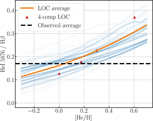
cloudy results of He iλ5876/H β for different He/H but at fixed Z = 3 Z⊙. The orange curve shows the weighted average for the line intensity ratios for individual one-zone models (in blue), ranging from 19 < log ϕ < 21 and 9 < log nH < 11, where the weight is given by a Gaussian distribution centred at log nH = 10, log ϕ = 19.5, with a standard deviation |$\sigma = 0.5~\rm dex$| in both nH and ϕ. The shade of the curves corresponds to the weight of the average. The red triangles are the result of a 4-component LOC model with Zα = 3 Z⊙, as shown in Table 1.
How reliable are these inferences? Table 2 gives the He iλ5876 intensity for the four component models of the simple LOC model. The He iλ5876/H β ratio for solar metals and He/H = 0.10 ranges from 0.102 for (log nH, log ϕ) = (10, 19) to 0.157 for (11, 20). Higher density in particular tends to give stronger He iλ5876. Could much of the BLR involve gas under conditions that enhance He iλ5876? Fig. 3 shows the He iλ5876/H β ratio for one-component cloudy models over a range of nH and ϕ, computed as described above. Here, we adopt a stopping column density of |$N_{\rm H}=10^{23}~\rm cm^{-2}$|. But for models with high ionization parameters (log U ≳ −0.5), the choice of stopping column density can affect the He iλ5876/H β ratio, due to the truncation of H + Strömgren sphere at |$N_{\rm H}=10^{23}~\rm cm^{-2}$|. For example, the model (log nH, log ϕ) = (10, 20) with solar metals and He/H = 0.10 gives He iλ5876/H β = 0.128 when |$N_{\rm H}=10^{23}~\rm cm^{-2}$|, but the same model with |$N_{\rm H}=10^{24}~\rm cm^{-2}$| gives He iλ5876/H β = 0.103. In addition, for even higher ionization parameters (log U ≳ 0), both H+ and He + Strömgren sphere are not complete at |$N_{\rm H}=10^{23}~\rm cm^{-2}$|, resulting in a low He iλ5876/H β ratio (as shown in the bottom-right corner of Fig. 3). The LOC average (see Fig. 2), on the other hand, is not hugely affected by the choice of NH, as it spans a range of ionization parameters. The contours in Fig. 3 also show that, for a helium abundance by number of He/H = 0.10, the intensity ratio ranges from 0.05 to 0.35, encompassing the full range of observed values. However, the He i emission comes from the bulk of the ionized volume. Any one-zone model for the He i emission must give realistic intensities for other lines that largely arise in the same zone, including C iii] and C iv. Fig. 4 shows log C iii]1909/C iv1549 for the same models as Fig. 3. Observed values typically fall in the range of −0.2 to −0.5. The figure shows that values in this range occur in a wedge-shaped region region, centred around log nH = 9.6 and log ϕ = 18.3, along with two narrow arms extending to high nH and ϕ. However, these upper arms are not realistic regarding other features of the BLR spectrum. In the upper left arm, C iii] is weak relative to H β due to collisional de-excitation at high density, and C iv is weak due to a low ionization parameter U. This region also overproduces low ionization lines such as Mg ii. Such considerations eliminate the parameter space giving the highest and lowest values of He iλ5876/Hβ.

cloudy model for He iλ5876/H β intensity ratio with stopping column density |$\log N_{\rm H} = 23~\rm cm^{-2}$|, Zα = 3 Z⊙, and |$\rm He/H=0.1$| by number. The ionizing flux varies from 17 < log ϕ < 21 and density varies from 9 < log nH < 12. The grey dotted lines show the ionization parameter, log U. For a given ionizing flux, the He i 5876/H β intensity ratio increases for higher density.
![Same as Fig. 3, but for log [I(C iii]λ1909)/I(C ivλ1549)]. The observed value is around −0.5 to −0.2.](https://oup.silverchair-cdn.com/oup/backfile/Content_public/Journal/mnras/525/4/10.1093_mnras_stad2642/1/m_stad2642fig4.jpeg?Expires=1750431624&Signature=4Qo9Fc0Rjvio6o3SLA6YV6HoL4lumyocN0nS9OgzGGCM9w4wfG7KKhFUO1I-lahqAXGmjFM-ckvwIL1fnvoxkfq5YMMMt0gpRXqCp7vwclQB6mlYrBMfKFKkn6ZlWszUCwR7XTJ7~oN4V73R-CLBuG8QSYS-Acxec1GRWIXic6TchE56cuTv-LCxPumhalypfqDTatcsyjo-pY-ldQmcRDj5P47XLqTqwi12vtqSt8V8yd5FCbKGI-bLYd-6gy-~PBAejNqJ9aCjL-Ojrf6qwgHs~ndXn8bta1Gk1YtY4FZstDdKGC3UIFc6yW3MPpIrsOCvclMHxvifItEkasiBAA__&Key-Pair-Id=APKAIE5G5CRDK6RD3PGA)
Same as Fig. 3, but for log [I(C iii]λ1909)/I(C ivλ1549)]. The observed value is around −0.5 to −0.2.
Four-component LOC (see 3.3.1) results for He iλ5876, H β intensities (in |$\rm erg\, cm^{-2}\, s^{-1}$|), and line intensity ratio I(He i λ5876)/I(H β) for Zα = Z⊙, |$\rm He/H=0.1$| by number.
| log nH | log ϕ | log I(He i λ5876) | log I(H β) | ratio |
|---|---|---|---|---|
| 10 | 19 | 5.984 | 6.973 | 0.102 |
| 10 | 20 | 6.982 | 7.876 | 0.128 |
| 11 | 19 | 6.184 | 7.094 | 0.123 |
| 11 | 20 | 7.205 | 8.009 | 0.157 |
| log nH | log ϕ | log I(He i λ5876) | log I(H β) | ratio |
|---|---|---|---|---|
| 10 | 19 | 5.984 | 6.973 | 0.102 |
| 10 | 20 | 6.982 | 7.876 | 0.128 |
| 11 | 19 | 6.184 | 7.094 | 0.123 |
| 11 | 20 | 7.205 | 8.009 | 0.157 |
We may also ask whether the AGN with the strongest He I lines have any indication of unusual physical conditions. Shang et al. (2007) give line intensities in the rest frame optical and ultraviolet for 22 broad line AGN. The data show no significant trend in the C iii]/C iv or the Mg ii/H β ratio as a function of He iλ5876/H β, which argues against a systematic difference in physical conditions for objects with especially strong He I emission.
The above considerations argue against high density as the cause of the occasional large He iλ5876/H β values, and we therefore entertain the possibility of a high helium abundance. The strongest observed values of He iλ5876/H β are 0.30 or slightly higher. The LOC results quoted above give He iλ5876/H β = 0.30 for He/H = 0.27. Conventional galactic chemical evolution cannot account for such a high abundance of helium. If we adopt a metallicity of 3Z⊙ (see above), then a helium abundance He/H = 0.11 would be implied by the primordial value He/H = 0.083 together with a Galactic enrichment ratio (expressed in terms of the mass fraction) of |$\rm \Delta Y/\Delta Z = 1.75$| (see equation B1). Most of the helium enhancement in the highest helium AGN must therefore come from some process that can produce a large amount of helium with a relatively small yield in heavier elements. We discuss below the prospect that SEPAD may provide such a process.
3.6 The Fe/Mg ratio
The abundance of iron in the BLR has received much attention, not least because the highest redshift quasars approach a time when Fe production by SN Ia is problematic (see Section B-A1 and A2). The Fe ii emission, especially in the optical, differs dramatically from object to object. Theoretical efforts to explain the intensity of Fe ii involve a complex model of the |$\rm Fe^{+}$| ions with many energy levels and transitions. The work of Wills, Netzer & Wills (1985) showed that fluorescence between different transitions has an important effect, along with collisional excitation and continuum fluorescence. The recent work of Sarkar et al. (2021), using the latest Fe ii atomic data sets in cloudy, largely succeeds in reproducing the optical and UV multiplet intensities observed in AGN.
Studies of the iron abundance in the BLR and its redshift dependence have largely focused on the ultraviolet Fe ii/Mg ii ratio. The Mg iiλ2800 line and the UV Fe ii bands around 2400 Å are close in wavelength and involve similar stages of ionization. These studies generally find that Fe ii/Mg ii depends little, if at all, on redshift (Maiolino et al. 2003; Verner et al. 2009; De Rosa et al. 2011; Schindler et al. 2020; Yang et al. 2021; Wang et al. 2022). However, caution is warranted for several reasons. In the recent photoionization models by Sarkar et al. (2021), as Fe/Mg varies from 0.1 to 10 times solar, the Fe ii (UV)/Mg ii ratio only increases by ∼0.4 dex, i.e.
Subtle trends in the line ratio could imply substantial trends in abundance. The emission in Fe ii(UV) comes from deeper in the photoionized clouds than does Mg ii (e.g. fig. 7 of Sameshima et al. 2017), making the ratio potentially sensitive to details of the BLR cloud structure. The Fe ii/Mg ii line ratio varies with Eddington ratio, approximately as |$\lambda _{\bullet }^{0.3}$| (Sameshima et al. 2017; Shin et al. 2021). Other parameters, such as microturbulence, also affect the Fe ii/Mg ii ratio (Sarkar et al. 2021). Furthermore, the sensitivity of the Mg ii line to Mg/H is greater than the sensitivity of Fe ii to Fe/H; in our one-slab cloudy models, Fe ii/Mg ii varies as (Fe/Mg)0.7 when only Mg/H is varied. Thus, the Fe ii/Mg ii ratio cannot be interpreted in isolation.
Another issue is the choice of template used to fit the Fe ii blends in the spectrum. The empirical template by Vestergaard & Wilkes (2001) (VW01) is set to zero under the Mg ii line, where Fe ii could not be measured. Several recent authors have used the template by Tsuzuki et al. (2006) (T06), which uses theoretical spectra to fill in the Fe ii emission under Mg ii. This reduces the Mg ii intensity and increases Fe ii/Mg ii. Schindler et al. (2020) give a detailed discussion. All of the measurements discussed here use the T06 template or make some other allowance for Fe ii emission under the Mg ii line.
In Table 3 and Fig. 5, we show averages of published measurements of Fe ii/Mg ii in several redshift bins. We have adjusted the observed values of Fe ii/Mg ii to a common fiducial Eddington ratio of log λ• = −0.55, using a slope Δlog (Fe ii/Mg ii) = 0.3 Δlog λ• from Sameshima et al. (2017). This adjustment, which was applied to individual quasars before averaging over redshift bins, is particularly important for the low redshift samples, Shin et al. (2021) give results for 29 low redshift AGN (zγ < 0.367) with archival HST spectra. Of these, the thirteen with log λ• > −1.5 have an average Fe ii/Mg ii = (2.88, 4.17), respectively (before, after) correction to the common Eddington ratio. For the brightest four objects, with log λ• > −0.5, the corresponding values are (3.80, 3.63). For a moderate redshift sample, we used the data base of spectral measurements by Shen et al. (2011) for SDSS DR7 quasars (see also Shin et al. 2021). For 69 202 quasars at 0.7 < zγ < 2.3, the mean Fe ii/Mg ii is (3.13, 3.60). At higher redshift, Dietrich et al. (2003) give an average Fe ii/Mg ii of 4.62. (We have applied the 10 per cent adjustment estimated by Dietrich et al. 2003, to allow for Fe ii emission under the Mg ii line. These values are not adjusted to our fiducial Eddington ratio because the authors do not quote values of λ•, but the correction is likely small for these bright quasars.) We have divided the measurements by De Rosa et al. (2011) into two redshift bins. The average of the three high redshift studies is Fe ii/Mg ii = 4.2, after adjustment for λ•. This agrees within ∼0.1 dex with the results at lower redshift. Given the dependence of Fe ii(UV)/Mg ii as |$(\rm Fe/Mg)^{0.2}$|, the corresponding limit on any redshift dependence of Fe/Mg is about ±0.5 dex.
![Redshift evolution of the BLR iron abundance. The open circles correspond to the inferred iron abundances [Fe/Mg] using fig. 11 in Sarkar et al. (2021). The closed circles are the inferred iron abundances using the adjusted line ratio Fe ii/Mg ii with the Eddington correction in Sameshima et al. (2017). Dietrich et al. (2003) do not have data for the Eddington ratio, so we use the uncalibrated Fe ii/Mg ii to calculate [Fe/Mg].](https://oup.silverchair-cdn.com/oup/backfile/Content_public/Journal/mnras/525/4/10.1093_mnras_stad2642/1/m_stad2642fig5.jpeg?Expires=1750431624&Signature=lvrtgx9MPCYm07gzC5fWJN6bxV8Yiu-v~AnV1hgSiOw2IKILLRddWVatqr2nO4uxvrVtt1eAmgJLjeCcuFqnIxOKOmXkehUyxAze7UqkqZjNZqDIhU-Wng9nulolho6nlKCsWC6AcV0S4Ilt93WcE9ZzDnU26bNTWPepU-zTxzdh0qxftfHqfPr7KL-AQu~OUT-6OTvTpEfSV7hjyjzk32wQ6K-OiTI3OCSbjTMhd2SAC~XnoNAN10eNa4e4kK2YZWJqoyABSDqZx6UiiSoS6YcAaVyq25CdEKclIQ4BpSC9-pD8v9hf4dxSLOqPulLJrmzuCQ2ZMiyl06JXym2QDA__&Key-Pair-Id=APKAIE5G5CRDK6RD3PGA)
Redshift evolution of the BLR iron abundance. The open circles correspond to the inferred iron abundances [Fe/Mg] using fig. 11 in Sarkar et al. (2021). The closed circles are the inferred iron abundances using the adjusted line ratio Fe ii/Mg ii with the Eddington correction in Sameshima et al. (2017). Dietrich et al. (2003) do not have data for the Eddington ratio, so we use the uncalibrated Fe ii/Mg ii to calculate [Fe/Mg].
The mean value of Fe ii/Mg ii ratio across redshift bins. The second column shows the mean observed value, and the third column shows the adjusted value by applying equation (12) in Sameshima et al. (2017) with each object’s Eddington ratio. For the low redshift objects in Shin et al. (2021), we also listed the mean Fe ii/Mg ii for four high-Eddington ratio objects (log λ• > 0.5) to make a better comparison for the high redshift objects.
| redshift | (Fe ii/Mg ii)obs | (Fe ii/Mg ii)adj | No. objects | Reference |
|---|---|---|---|---|
| zγ < 0.367 | 2.88 (3.80) | 4.17 (3.63) | 13 (4) | Shin et al. (2021) |
| 0.7 < zγ < 2.3 | 3.13 | 3.60 | 69 202 | Shen et al. (2011) |
| 4.5 < zγ < 4.7 | 4.62 | – | 5 | Dietrich et al. (2003) |
| 4.5 < zγ < 5.1 | 2.95 | 2.84 | 10 | De Rosa et al. (2011) |
| 5.7 < zγ < 6.4 | 4.56 | 4.37 | 28 | Wang et al. (2022) |
| 5.8 < zγ < 6.4 | 3.03 | 2.44 | 14 | De Rosa et al. (2011) |
| 5.9 < zγ < 6.9 | 5.47 | 5.11 | 32 | Schindler et al. (2020) |
What is the actual value of Fe/Mg that corresponds to this redshift-independent line ratio? Let us consider the highest 3 redshift bins in Table 3, with an average Fe ii/Mg ii = 4.2. For this value, fig. 11 of Sarkar et al. (2021) gives Fe/Mg of 0.27 times solar (for the De Rosa et al. 2011 integration range). That figure, however, is for solar abundance (except for iron). For our adopted alpha-element abundance of three times solar, adjustments must be made. The cloudy models underlying fig. 11 of Sarkar et al. (2021) use log ϕ = 20 and log nH = 11, giving log U = −1.5. In our cloudy models, these parameters give Mg ii/H β in agreement with typical observed values ∼1.7 (based on the composite spectrum of Vanden Berk et al. (2001) and the sample of SDSS quasars described above.) However, when all heavy elements, including iron, are increased together, Mg ii/H β increases and Fe ii/Mg ii decreases. In order to restore agreement for Mg ii/H β, the ionization parameter must be increased. In our cloudy models, a reduction in density to log nH = 10.5, giving log U = −1.0, achieves this. These parameters raise Fe ii/Mg ii by about 0.05 dex, and then equation (4) requires a reduction of Fe/Mg by 0.25 dex to restore agreement for Fe ii/Mg ii. The result of this analysis is [Fe/Mg] =−0.8 ± 0.5, using the above uncertainty range. For an alpha-element abundance of three times solar, we then have [Fe/H] =−0.3 ± 0.5. This rules out a Pop II value of Fe/H, but it is compatible with a Pop II (i.e. SN II) value of Fe/Mg.
This result, however, is based on a single photoionization model with a particular nH and ϕ. How might the result change for a mix of parameters as envisioned by the LOC model? Suppose that the mix contains some highly ionized gas that emits much of the radiation in C iv, O vi, etc. as well as much of the observed H β. Then, the bulk of the Mg ii and Fe ii must come from a component with a high value of Mg ii/H β, so that the mix gives the observed ratio. As an example, consider a low-ionization component that has log U = −1.5 as discussed above but with Zα = 3 Z⊙. For these parameters, in our cloudy models, Fe ii/Mg ii is now 0.13 dex lower (at fixed Fe/Mg) than for solar metals. By equation (4), we now must raise the above value Fe/Mg = 0.27 from fig. 11 of Sarkar et al. (2021) by 0.65 dex to fit the observed value of Fe ii/Mg ii, resulting in Fe/Mg = 1.2(Fe/Mg)⊙. Thus, simply having Mg ii and Fe ii come from a region of modestly lower ionization parameter leads to a much larger value of Fe/Mg. This suggests that the values of Fe/Mg and Fe/H derived in the preceding paragraph should be considered lower limits, and it illustrates the need for caution in deriving an iron abundance from the UV Fe ii emission.
3.7 Comparison of NLR and BLR
The region emitting the narrow emission lines of AGN (Narrow Line Region or ‘NLR’) affords an opportunity for comparison of BLR abundances with interstellar abundances in the core of the host galaxy but outside the accretion disc. The NLR has a radius of order 100 pc for moderate luminosity AGN and scales roughly as |$L_{\rm AGN}^{1/2}$| (Bennert et al. 2006). (This refers to the radius containing the bulk of the emission, not the outermost boundary.) For a density |$n_e = 10^4~\rm cm^{-3}$| (e.g. Terao et al. 2022), the mass of emitting gas is of order 104 or 105 M⊙. This is much larger than the mass of emitting gas in the BLR but less than the mass of the accretion disc or the stellar mass located at the radius of the NLR (see Section 2).
Studies of abundances in the NLR have increased in recent years, but uncertainties remain. The NLR has typical gas densities ranging from 103 to |$10^6~ \rm cm^{-3}$|. While these densities are much lower than in the BLR, they still exceed the critical densities of many of the forbidden lines observed in the optical and neighbouring wavelength bands. This makes it difficult to derive electron temperatures from the forbidden line ratios often used in nebular studies, and this in turns impedes direct determinations of abundances. Consequently, photoionization models are needed. Because the narrow lines are difficult to measure in broad line objects, especially in the ultraviolet, such studies have often targeted narrow line objects (Seyfert 2 or QSO 2). The results are assumed to apply to the NLR of broad line objects, in a statistical sense, on the basis of the unified model of AGNs.
Nagao et al. (006b) carried out a photoionization model study of narrow line AGN in the redshift range zγ = 1.2 to 3.8, using rest-frame ultraviolet lines, in particular He ii, C iii], and C iv. They found that the observations were consistent with a low density (|$10^3~\rm cm^{-3}$|) NLR with subsolar abundances (0.2–1.0 Z⊙ or a high density model with results ranging from subsolar to super-solar (0.2–5 Z⊙). In either case, there was no indication of evolution with redshift (see also Matsuoka et al. 2009). Mignoli et al. (2019) studied a large sample of Type 2 AGN at redshift 1.5 to 3.0 with the aid of photoionization models. The results, averaged over three redshift bins, show a progressive decrease with increasing redshift: 12 + log O/H = 8.55, 8.34, 8.16 at zγ = 1.7, 2.2, 2.9, respectively. In contrast, Terao et al. (2022) analyse rest-UV spectra of 15 narrow line radio galaxies at redshift 3, including a number of fainter emission lines that help to constrain photoionization models. They find NLR abundances in the range Zα = 0.6 to 2.1 Z⊙, with an average of 1.2 Z⊙. Dors et al. (2020) report solar or modestly subsolar oxygen abundance for low redshift SDSS narrow line AGN, derived from a variety of semi-empirical calibrations of the strong lines ([N ii] and [O iii]). Aside from individual outliers, these studies do not find NLR alpha abundances similar to the high values found for the BLR. In addition, Du et al. (2014) report a positive correlation between N v/C iv in the BLR and [N ii]/H α in the NLR, implying a strong correlation between NLR and BLR metallicities. This correlation can be explained by the metal-rich gas in the BLR being transported to the NLR due to outflow Du et al. (2014).
The abundance of iron in the NLR can be derived from the intensity of the emission-line ratio of [Fe vii] λ6087 to [Ne v] λ3425 (Nussbaumer & Osterbrock 1970). This line ratio was measured by Shields, Ludwig & Salviander (2010) in composite spectra of low-redshift SDSS quasars (zγ ≈ 0.3) grouped into 5 bins by increasing strength of the broad Fe ii emission. Their results give an average value of [Fe vii]/[Ne v] = 0.34, with a scatter of only 10 per cent among the bins and no discernible trend with broad Fe ii strength. We ran plane-parallel cloudy models for the NLR with solar abundances, log nH = 3 or 5 (Nagao et al. 006b), log U = −0.98 or −1.98, and a stopping electron temperature of 3000 K. In terms of the choice of the ionization parameters, the observational results for 15 objects in (Terao et al. 2022) give −2.0 ≲ log U ≲ −1.0. Pérez-Montero et al. (2019) gives −2.42 ≲ log U ≲ −1.27 for the NLR. In addition, reverberation mapping result (Peterson et al. 2013) shows that the majority of the emission from NLR comes from its inner region (|$R_{\rm NLR}\sim 1-3 \rm pc$|). This first and hitherto only measurement provides the estimated NLR size, independent of those inferred from spatially resolved imaging and spectroscopy (Cackett et al. 2021). This indicates that, within the same AGN, the ionizing flux NLR sees is ∼106 times smaller than in the BLR. Combining with log nH = 5, we get log U ∼ −1.98. The four models gave iron abundance ranging from (Fe/Ne) = 0.85 to 1.55 (Fe/Ne)⊙. We conclude that the Fe-to-α ratio in the NLR of typical low-redshift quasars is close to the solar value. This result and the average line ratio used here are consistent with Nagao et al. (2003). From their photoionization modelling, we estimate an uncertainty of ±0.2 dex in the derived Fe/Ne ratio. Our value of Fe/Ne is consistent with our derived value of Fe/Mg in the BLR, within the large error bar of the latter.
An interesting case is that of the ‘nitrogen loud’ AGNs, which have exceptionally strong lines of N v, N iv], and N iii] from the BLR, suggestive of very high metallicity and secondary nitrogen production. These objects are only a small fraction of the AGN population (e.g. Batra & Baldwin 2014; Maiolino et al. 2023). Matsuoka et al. (2017) use the equivalent width of [O iii] to argue that N-loud AGN have approximately solar metallicity in their NLR (see also Araki et al. 2012).
In summary, results for the NLR indicate subsolar or around solar abundances, with a possible decrease toward higher redshift. There is little indication in the NLR of abundances resembling the high (≥4 Z⊙) values found for the BLR. Furthermore, the extreme nitrogen abundances shown by the broad lines of some objects appear not to be reflected in their NLR, at least regarding the alpha-elements. These results support the idea that the extreme metal enrichment of the BLR has its origin in the immediate vicinity of the accretion disc.
4 SUMMARY AND DISCUSSIONS
In comparison with the Galactic chemical evolution model (Appendix B), we interpret their implication of the AGNs’ abundance in terms of the SEPAD model (Sections 2, 4.2, Appendix B).
4.1 A brief observational synopsis
The chemical evolution of the Galactic disc and halo is constructed based on the spectroscopy of populations I and II stars. The |$[\alpha /\rm H]$| and [Fe/H] in these stars correspond to their values in the ISM at their formation epochs, which extend over several Gyr (Section B). Similarly, the abundance of the α and Fe-peak elements in AGNs with overlapping range of ages (zγ = 0 − 7), is measured from their BLRs which are analogous to the ISM in the Galactic context (Section 2).
A) α-element abundance.
A1. The most important and robust observational constraint is the lack of evolution in BLRs’ super-solar [α/H] (≃ 0.5 or Zα|BLR ≃ 0.06), i.e. its constancy through the cosmic epochs zγ(∼ 0–7) (Section 3.2).
A2. The N/(O + C) ratio is elevated from the solar value. N-loud AGNs may represent a small fraction of exceptions (Section 3.3).
A3. Although some ratios of BLR α lines appear to vary with M• and λ• = L•/LE• (Xu et al. 2018), these dependencies can be attributed to emission-line physics rather than actual BLR [α/H] variations (Temple et al. 2021).
A4. As a population, [α/H] for the NLR also appears to be zγ independent and smaller by ≲0.5 (i.e. [α/H] ≃ 0 or Zα|NLR ∼ 0.02) than that for the BLR (Section 3.7). BLRs’ [α/H] is also uncorrelated with signatures of star formation in the host galaxies (Simon & Hamann 2010).
B) Helium abundance. The galactic chemical evolution leads to minor increases in the Helium mass abundance from the big bang Y0 ≃ 0.245 with Zα, 0 = 0 and X0 ≃ 0.755 (Carigi & Peimbert 2008; Peimbert et al. 2016; Valerdi, Peimbert & Peimbert 2021) to today YG ≃ 0.28 (Arnett 1996) with ΔYG = YG − Y0 ≃ 0.04 and ΔZα, G = Zα, G ≃ 0.02 so that ΔYG ∼ 1.8ΔZα, G (equation B1).
B1. By number, AGNs’ average [He/H] ∼0.114 and in exceptional objects may reach 0.4 for their BLRs (Section 3.5, Fig. 6). The corresponding Y = 0.32, ΔY = Y − Y0 ∼ 0.08 which is slightly smaller than that 1.8Zα|BLR ∼ 0.09 or ΔYG + 1.8ΔZα ∼ 0.1 extrapolated from the BLR’s Zα|BLR, NLR’s Zα|NLR, and their difference ΔZα(≃ Zα|BLR − Zα|NLR ≃ 0.035) with the standard stellar and Galactic chemical evolution models (equation B1). The corresponding [ΔY] = log(ΔY/ΔYG) ≃ 0.36.
B2. Within the measurement uncertainties, [He/H] ∼0.08 ± 0.04 by number and [ΔY] ∼ 0.25 ± 0.1 by mass for the NLR (Dors et al. 2022).
![Summary of abundance by elements in the BLR (in blue) and NLR (in red). ΔY is the enrichment in the AGN helium abundance relative to the primordial helium abundance, normalized by the enrichment in the solar helium abundance, ΔYG. The open blue circles represent the inferred helium abundance in the objects with extreme He iλ5876/H β values (e.g. 3C120), and the error bars for the extreme Helium abundance corresponds to the modelling error, so the actual error is larger than the error indicated in the plot. The value of [(C+N + O)/H] in the BLR is inferred from the average line intensity of (Si iv + O iv])/C iv in Lai et al. (2022) with C iv blueshift less than $1500 \rm \, km\, s^{-1}$. For the NLR, [(C+N + O)/H] is the average value of the α-element abundance in Terao et al. (2022). The value of [N/H] in the BLR is inferred from the line intensity ratio of N iii]/O iii]. For the NLR, [N/H] is inferred from [N ii]/[O iii] ratio (Dors O. L. et al. 2017).](https://oup.silverchair-cdn.com/oup/backfile/Content_public/Journal/mnras/525/4/10.1093_mnras_stad2642/1/m_stad2642fig6.jpeg?Expires=1750431625&Signature=GzDYn51xGBjV8EUyPKk7kszKJHLkW4lXo8XVYhHwlTKWiBS66V2i8PWJhoADxRHrkLw42TCpA4n987OP-LizCZASzJMvyV5-38VaFO-33Su6dLT6yVRfPbYQBpsPz69nRTbLjCu4FmQvANcyRU25snX5qZilUluZwdfueIvoQQsAzIa8uttt7OFNVaxYqzOMztCMF1KNXdqpBAIeRmLGUme-yQjnSuHSWFgLfas6vIoN6laYhkcZKlAtcFwjN7Cbc6bwnKefcpB2mksmZ98AmmomUnGwDodYzdrkEDi-pFjuGmafTXgX5ImibWa0HhM88SznuDWp99RCHz2to8-Jqg__&Key-Pair-Id=APKAIE5G5CRDK6RD3PGA)
Summary of abundance by elements in the BLR (in blue) and NLR (in red). ΔY is the enrichment in the AGN helium abundance relative to the primordial helium abundance, normalized by the enrichment in the solar helium abundance, ΔYG. The open blue circles represent the inferred helium abundance in the objects with extreme He iλ5876/H β values (e.g. 3C120), and the error bars for the extreme Helium abundance corresponds to the modelling error, so the actual error is larger than the error indicated in the plot. The value of [(C+N + O)/H] in the BLR is inferred from the average line intensity of (Si iv + O iv])/C iv in Lai et al. (2022) with C iv blueshift less than |$1500 \rm \, km\, s^{-1}$|. For the NLR, [(C+N + O)/H] is the average value of the α-element abundance in Terao et al. (2022). The value of [N/H] in the BLR is inferred from the line intensity ratio of N iii]/O iii]. For the NLR, [N/H] is inferred from [N ii]/[O iii] ratio (Dors O. L. et al. 2017).
(C) Fe-peak abundance. In the Galaxy, old stars with ([α/H] ≲ −2) have sub-solar [Fe/Mg] (∼−0.3 − 0) and population I stars (with [α/H] ∼0) have solar or super-solar [Fe/Mg] (∼0 − 0.2). Since Mg is an α element, this correlation also extends to [Fe/α] and it has been interpreted to indicate that the Fe production was mostly due to SN ii when the Galaxy was young and pristine, whereas the present-day Fe content is mainly released from SN ia, which took time to evolve (Section B).
C1. AGNs’ slightly sub-solar [Fe/Mg] (∼−0.8–0.1) is inferred from the broad Fe ii/Mg ii lines (Section 3.6).
C2. BLRs’ nearly solar [Fe/H] (with a mass fraction ZFe ∼ 10−3) is inferred from their [Fe/Mg], calibration of solar α-element-abundance distribution (see above), and super-solar [α/H] (Section 3.2).
C3. The combination of sub-solar [Fe/Mg] (C1) with super-solar [α/H] (A1) for the BLRs does not match that for the Galactic stars (Section B).
C4. The inferred [Fe/H] for BLR is independent of zγ.
(D) Observational uncertainties.
There are some less well-established pieces of evidence on:
weak, if any, dependence of α element abundance on the SMBHs’ mass and AGNs’ Eddington ratio (A3) and
minor evolution in [Fe/Mg] or [Fe/α] element (Fe/Mg) ratio in BLR of low-red shift AGNs.
There is little or no data on:
[He/H] over a wide range of zγ and
[Fe/H] for NLR.
Large observational uncertainties are associated with:
insensitive dependence of Fe ii/Mg ii on [Fe/α] and
discrepancies of N/O versus N/C in different lines.
4.2 Some implications on SEPAD
The two salient features of this SEPAD scenario (Section 2) are (1) the prolific production of super-solar α-element and solar Fe abundances at high-zγ and (2) the constancy of these abundances since zγ ∼ 7 (i.e. more than 12 Gyr ago). With the observed data (Section 4.1), we gather supporting evidence and place some constraints on the SEPAD model.
A. Adequate auxiliary power for outer regions of AGN discs. The SEPAD model is motivated by the possible auxiliary power, due to thermonuclear burning inside the embedded stars, to exceed the energy dissipation rate of the accretion flow. For a M• = 108 M⊙ SMBH, this transition occurs at a radius (∼3 light days) ≲ that inferred for the BLR (Horne et al. 2021; Lobban & King 2022). Since the polluted BLR is downstream in the accretion-disc flow (i.e. closer to the SMBH) from the sites where He, α, and Fe elements are being injected into the disc, their stellar sources’ |$Q^+ _\star$| dominates their local |$Q^+ _\nu$|. In a thermal equilibrium, the supplemental |$Q^+ _\star$| leads to extra infrared excess which is commonly observed in AGNs’ SED (Sanders et al. 1989). This inference is supported by the half-light radius of AGN discs extrapolated from microlensing observations (Pooley et al. 2007; Morgan et al. 2018; Cornachione et al. 2020), which appears to be larger than that derived based on the standard steady-state viscous accretion disc model.
B. A population of massive MS stars in AGN discs. SEPAD models predict a population of MS stars with masses (m⋆ ∼ 102–3 M⊙) to maintain an accretion-wind equilibrium. Their nearly Eddington-limited luminosity is powered by the conversion of H into He at a rate |${\dot{M}}_{\rm He}$| (Section 2). The observed super-solar [ΔY] > 0 in high-zγ (∼5–7) AGNs (Section 4.1-B1) supports the expectation of rapid (in ≲1 Gyr) He enrichment beyond that of normal galactic chemical evolution. The mean value of ΔY ≲ 0.08 for most AGNs is less than the H-to-He conversion rate (|${\dot{M}}_{\rm He}/{\dot{M}}_{\rm d} \sim 0.15$|) required to account for the auxiliary power such that some of the He-byproducts during the embedded stars’ MS evolution may have been converted into α or Fe elements (Section 4.2-C) or be deposited into rBHs (Section 4.2-F).
C. Embedded stars’ transition from MS to PostMS evolution. An outstanding issue is whether H fuel in massive stars is continually replenished by a fresh supply of disc gas so that they remain on the MS indefinitely or it is exhausted in the CNO burning zone, which would lead to transition to PostMS evolution (Section 2). Since He is converted into α elements during the PostMS evolution, the detection of strong signatures of super-solar Zα (Section 4.1-A1) with weak or no dependence on λ• and M• (Section 3.2, 4.1-A3) clearly indicates that this transition has taken place during the active AGNs’ active phase in contrast to the scenario that massive stars evolve off the MS after the disc depletion (Cantiello et al. 2021). Moreover, the modestly positive observed value of [Y] (Section 4.1-B2) also implies that these stars are embedded in He-enriched (but not He-predominant) disc gas such that their MS-to-PostMS transition cannot be due to the severe He pollution over wide regions of AGN discs as suggested by Jermyn et al. (2022). The quenching of H replenishment requires either an efficient confinement and retention of the stellar wind with He-byproducts or the prevention of compositional mixing by a radiative zone between the recycled gas and the nuclear-burning core (Ali-Deb, Cummings, and Lin in preparation). The modest |$\Delta Y_{\rm d} (\sim 0.08 \lt {\dot{M}}_{\rm He}/{\dot{M}}_{\rm d}\sim 0.15$| (Section 4.1-B1) is consistent with the SEPAD model with evolving (with lifespan τ⋆ ∼ 4–5 Myr rather than ‘immortal’) stars provided a major fraction of the He-byproduct during massive stars’ MS evolution is retained and recycled (analogous to a close-box model), converted into α, Fe and released to the disc during their PostMS evolution and subsequent SN explosions.
D. Mass-loss during embedded stars’ PostMS evolution. The observed [α/H] (Section 4.1-A1) is comparable to the value of Zα inferred, based on the SEPAD scenario, for the α-element production during the PostMS evolution of N⋆ ≳ 103 − 4 coexisting embedded stars within a few pc. This agreement also implies that most of the α-byproducts are released to the disc along with the He-byproducts such that the embedded stars had substantial mass-loss along their evolution track and their pre-collapse cores have downsized to range ≲15 M⊙ before their SN ii explosion (Sukhbold et al. 2016).
E. Fe production from core-collapse SN ii in AGN discs. The observed [Fe/H] ∼0 (Section 4.1-C2) corresponds to ZFe ∼ 10−3 and a rate of Fe release into the disc at a rate |${\dot{M}}_{\rm Fe} \sim Z_{\rm Fe} {\dot{M}}_{\rm d} \sim 10^{-3} m_8 f_\bullet M_\odot \ {\rm yr}^{-1}$| (equations 1 and 2). The Fe is mostly released from SN ii with a fractional addition from the Fe production through the α-chain reaction during the PostMS evolution. The sub-solar [Fe/α] (Section 4.1-C1) is a signature of SN ii ejecta. Scaling with an yield of ΔMFe ∼ 0.1 M⊙ (Sukhbold et al. 2016; Rodríguez et al. 2021), we infer a typical rate of SN ii to be |${\dot{N}}_{\rm SNII} \sim 10^{-2} m_8 f_\bullet \ {\rm yr}^{-1}$| which is comparable to the rate N⋆/τ⋆ of massive star formation inferred based on the SEPAD scenario.
F. Birth of residual black holes rBHs in AGN discs. The collapse of stellar cores at the end of the PostMS evolution, leads to the formation of seed rBHs with a few M⊙. Their consumption of some residual He, α, and Fe in the collapsing cores can be used to account for the discrepancy between the expected conversion fraction in |$Y (\simeq {\dot{M}}_{\rm He}/ {\dot{M}}_{\rm d} \sim 0.15)$| produced by the auxiliary stellar power sources and that observed from the sum of ΔY ∼ 0.08 and ΔZα ∼ 0.035 (Section 4.1-B1, equation 3). Since self-regulated star formation and evolution lead to a stellar population with a top-heavy equilibrium mass function, the production rate of seed rBH is |$\sim {\dot{N}}_{\rm SNII}$|. Moreover, low-mass black holes accumulate and diffuse rather than migrate or flow with gas in the disc. These seed rBHs subsequently gain several-fold in mass through accretion and/or coalescence. These processes do not lead to further chemical evolution due to heavy-element production, albeit energy dissipation during accretion onto rBHs contributes to the auxiliary power. SEPAD scenario assumes that the rBHs become the seeds of merging black holes, which contribute to the sources for intense excitation of gravitational waves.
G. Multiple generations of embedded stars. Multiple generations of PostMS stars are needed to produce the observed high [α/H] (Section 4.1-A1). Moreover, the synthesis of α elements through the triple-α and α-chain reaction during the PostMS stage produces low [N/(C + O)] ratio (Section 4.1-A2). Its redistribution to the observed values of [N/(C + O)] requires elemental redistribution within the CNO cycle on the MS track of next-generation stars. This inference has implications on the AGN persistent time-scale (≳ τ⋆ a few Myr, Section 4.2-K) and the number of rBHs born in AGN discs (|$\sim N_{\rm rBH} \gtrsim {\dot{N}}_{\rm SNII} \tau _\star \sim 10^4 m_8 f_\bullet$|, Section 4.2-E & F).
H. In situ pollution in AGN discs. The SEPAD scenario implies the metallicity in the disc is higher than that being supplied to the disc. Under the assumption that the NLR is located either beyond the outskirt of the AGN disc or in the host galaxies, the observed higher values of BLR’s Yd and [α/H] than those of the NLR (Section 4.1-B2 and A4) provide a circumstantial evidence for SEPAD regardless of whether gas in the NRL is the diluted outflow from or fresh supply to that in the BRL. The absence of zγ-dependence in [α/H] and [Fe/H] (Section 4.1-A1 and C4) and super-solar [α/H] with sub-solar [Fe/α] (Section 4.1-C3) in AGNs’ BLRs (in contrast to the observed [α/H]–zγ and [Fe/α]–[α/H] correlations for the galactic chemical evolution Section B) also implies that they are not significantly affected by the enrichment or star-formation activities (Section 4.1-A4) of their host galaxies’ ISM.
I. Clearing of pollutants by accretion onto SMBHs. The observed zγ-independence of [α/H] and [Fe/H] (Section 4.1-A1 and C4) is in strong contrast to galactic chemical evolution Section B. But it is consistent with SEPAD’s inference that the pollutants released by the stars are mixed with the disc gas, advected inward, and continuously cleared into the central SMBHs.
J. Self-regulated star formation rate. The lack of (or weak if any) M• or λ•-dependence in the observed [α/H] (Section 4.1-A3) is in line with SEPAD’s inference based on the assumption of self regulate star formation rate (∼N⋆/τ⋆) and capture rate (Artymowicz et al. 1993; Goodman 2003; Thompson et al. 2005) in AGN discs. At any given radius, both the critical gas Σ and stellar surface density s⋆ required auxiliary power |$Q^+ _\star$| needed to maintain Q = 1 for marginal stability increases with M•. In high-Σ discs (with relatively high |${\dot{M}}_{\rm d}$|), more stars form, so the heavy element contamination is diluted. Thus, the [α/H] and [Fe/H] dependence on M• and |${\dot{M}}_{\rm d}$| essentially cancel with each other. Moreover, their dependence on the Eddington factor |$\lambda _\bullet (\propto {\dot{M}}_{\rm d} /M_\bullet)$| is correspondingly weak.
K. AGN persistent time-scale. The inference of multiple generations of embedded stars (Section 4.2-G) implies that the AGN disc must have persisted for at least τ⋆ (a few Myr). The observed sub-solar [Fe/α] also indicates that SN ia is not the predominant channel for Fe enrichment despite the super solar [α/H] (Section 4.2-E). This inference implies a limit on the embedded white dwarf population. Since their MS progenitors have M⋆ ≲ 8 M⊙ with a lifespan ≳5 × 10⁷ yr and additional time is needed for the white dwarf remnants to acquire sufficient (Chandrasekhar) mass to undergo collapse along with SN ia, the sub-solar [Fe/Mg] can be used to infer an upper limit on the typical AGN duration (≲a few 108 yr) and their discs do not extend significantly beyond a few pc (i.e. the typical distance of the ‘dusty torus’) from the SMBHs.
4.3 Some outstanding issues.
There are several uncertainties associated with the simplest version of the SEPAD model we have adopted in this paper.
A. Stellar mass spectrum and population. In the construction of the simplest SEPAD models, we assume the dominant power sources to be those MS stars with an equilibrium m⋆ and [He/H] of the disc gas. We need to take into account modification due to the L⋆–m⋆ for the MS stars with an evolving internal [He/H] and coexisting PostMS stars. Supernovae and accretion onto a growing population of rBHs also contribute to |$Q^+ _\star$| and therefore the star formation rate, although they do not directly affect the chemical evolution of the disc.
B. Main-sequence turn off. It is not clear whether an accretion-wind equilibrium can be stably maintained with a high retention and recycling efficiency. The possibility of non-spherical flow and interchange between inflow and outflow need further theoretical analysis.
C. Release of He, α, and Fe byproducts to the disc during PostMS evolution. Wind prescriptions affect PostMS-evolution models for embedded stars’ interior, He α conversion rate, α and Fe yield. They also lead to different values for pre-collapse core mass, neutron stars versus rBH remnants. The efficiency of the PostMS mass-loss needs further studies.
D. Stellar mergers. The coexistence of a large population (with N⋆ ≳ 103) of embedded stars raise the possibility of their collisions and coalescence. While the merger events would be followed by rapid downsizing and the return to the equilibrium mass, we need to check whether PostMS-star mergers may enhance the production and release rates of α and Fe byproducts.
E. Migration and relaxation of embedded stars. Although isolated embedded stars may migrate extensively over AGN discs, tidal interference by nearby cohorts may suppress this effect. Nevertheless, we need to examine whether modifications in the |$Q^+ _\star$| distribution may be offset by the local |$Q^+ _\star \simeq Q^-$| thermal equilibrium in self-regulating the star formation rate.
F. Radial extent of AGN discs. The disc’s mid-plane density, temperature, and embedded stars’ accretion rate decreases with their radius. Beyond a few pc, the equilibrium stellar mass also decreases below those of neutron-star or white-dwarf progenitors, although N⋆ also increases with R. Some constraints, based on the observed [Fe/α] ratio, may be inferred for the physical extent of the star-forming region in AGN discs.
Despite these uncertainties, this paper highlights the relevance and importance of AGNs abundance inference from their spectroscopic signatures in deciphering structure and evolution of their discs. The SEPAD scenario also predicts the occurrence of SN ii and production of rBH in AGN disc. Their potential observational signatures will be explored and discussed elsewhere.
ACKNOWLEDGEMENTS
We thank Gary Ferland, Andy Fabian, Stan Woosley, Yixian Chen, Mohamad Ali-Deb, Andrew Cumming, Jamie Law-Smith, Matteo Cantiello, and an anonymous referee for useful communications.
Funding for the Sloan Digital Sky Survey V has been provided by the Alfred P. Sloan Foundation, the Heising–Simons Foundation, the National Science Foundation, and the Participating Institutions. SDSS acknowledges support and resources from the Center for High-Performance Computing at the University of Utah. The SDSS web site is www.sdss.org.
SDSS is managed by the Astrophysical Research Consortium for the Participating Institutions of the SDSS Collaboration, including the Carnegie Institution for Science, Chilean National Time Allocation Committee (CNTAC) ratified researchers, the Gotham Participation Group, Harvard University, Heidelberg University, The Johns Hopkins University, L’Ecole polytechnique fédérale de Lausanne (EPFL), Leibniz-Institut für Astrophysik Potsdam (AIP), Max-Planck-Institut für Astronomie (MPIA Heidelberg), Max-Planck-Institut für Extraterrestrische Physik (MPE), Nanjing University, National Astronomical Observatories of China (NAOC), New Mexico State University, The Ohio State University, Pennsylvania State University, Smithsonian Astrophysical Observatory, Space Telescope Science Institute (STScI), the Stellar Astrophysics Participation Group, Universidad Nacional Autónoma de México, University of Arizona, University of Colorado Boulder, University of Illinois at Urbana-Champaign, University of Toronto, University of Utah, University of Virginia, and Yale University.
DATA AVAILABILITY
The data analysed in this paper can be found on the Sloan Digital Sky Survey (www.sdss.org).
References
APPENDIX A: Line intensity
The above discussion has made use of the (Si iv + O iv])/C iv emission-line ratio as an abundance indicator. In order to assess the robustness of this indicator, we have examined the photoionization physics responsible for the behaviour of these lines.
Nagao et al. (006b) popularized this indicator using photoionization model predictions based on the ‘LOC model’ for the BLR (see above). However, for an examination of the physics behind the behaviour of C iv and other lines, it is more practical to study the ionization structure of individual clouds. Therefore, we investigated a set of cloudy 17.01 models for single clouds with a slab geometry and the ‘Strong Bump’ ionizing continuum employed by Nagao et al. (006a). Our reference model had a hydrogen density nH = 1010, an incident ionizing photon flux ϕ = 1019, a stopping column density of 1023, and solar abundances. The ionization parameter of this model is U = 10−0.98.
In the models presented here, we assume that the ionizing UV photons are emitted from the innermost regions of the disc near the SMBHs. Since these regions are stable against gravitational instability, the energy sources of the ionizing photon are presumably associated with accretion onto the SMBHs or the disc corona. The SEPAD model suggests star formation occurs in gravitationally unstable outer regions of the disc (Paczynski 1978; Goodman 2003) beyond a few light days (|$\gt r_{\rm Q} \sim 0.06\ \alpha _\nu ^{2/9} m_8 ^{7/9}$| pc for typical AGNs) and the embedded stars sediment near the mid-plane (Artymowicz et al. 1993) where the gas density (|$\rho _{\rm c} \simeq 8 \times 10^{-16} m_8 r_{\rm pc}^{-3} {\rm ~g \ cm^{-3}}$| where rpc = R/pc) is much larger than that of the interstellar medium including giant molecular clouds and the mid-plane temperature |$T_{\rm c} \sim 800 {m_8^{5/12} \alpha _\nu ^{-1/6} r_{\rm pc}^{-3/4}} {\rm K}$| (see Section 2 for concept and derivation will be presented elsewhere). With nearly Eddington-limited luminosity, individual massive stars produce H ii regions whose Strömgren radii (|$R_{\rm s} \simeq 2 \times 10^{15} {r_{\rm pc}^{29/16} m_8^{-9/16}} {\rm cm}$|) are less than a few per cent of their Roche radii (M⋆/3M•)1/3R and the disc thickness H = hR where |$h\sim 0.02 r_{\rm pc}^{1/2} \alpha _\nu ^{-1/3} m_8 ^{-1/6}$|). Although they provide auxiliary power to maintain hydrostatic equilibrium in the direction perpendicular to the disc plane, their UV photons are absorbed well below the BLR, presumed to be at or just above the disc surface. The reprocessed radiation diffusing through the optically thick disc mainly serves to enhance the composite spectral energy distribution (SED) in the visual and IR continuum without significant modifications in the flux of ionizing photons. The X-ray and UV to optical and IR luminosity ratio is a function of the SMBH’s mass, the discs’ inner and outer radii, the Eddington ratio and it can be, in principle, fitted to match the observed SED (Sirko & Goodman 2003). This dependence introduces uncertainties in deriving the metallicity and Helium abundance directly from the equivalent width of the emission lines. However, abundance determination based on line ratios is less sensitive to the slope of the SED than the lines’ equivalent width. In order to facilitate comparison with previous studies, we adopt Nagao et al. (006a)’s approximate SED in the line-ratio analysis presented here (Section 3).
We ran a series of models with the above parameters and a metallicity of (0.5, 1.0, 2.0, 4.0, and 8.0) Z⊙. All heavy elements were varied in proportion (including nitrogen), with helium held constant at 10 per cent of hydrogen by number of atoms. The resulting line intensities are given in Table A1. As C/H increases a factor of 16, the C iv emission line, relative to H β, monotonically decreases by a factor 2 (see fig. 15 of Ferland et al. 1996). In contrast, O iv] remains roughly constant, and Si iv increases. As a result, (Si iv + O iv])/C iv increases a factor of ∼3. This resembles the trend shown in fig. 29 of Nagao et al. (006b). Between 0.5 and 8 Z⊙, our results give a dependence (Si iv + O iv])/C iv|$\propto Z_{\alpha }^{0.46}$|, whereas table 10 in Nagao et al. (006a) gives |$Z_{\alpha }^{0.44}$|. Also, at solar abundance, the ratio is 0.149 in Nagao et al. (006a)’s model, smaller than our result by 0.03 dex. This close agreement may be fortuitous, but it suggests that this indicator is not extremely sensitive to the BLR geometry, at least in the general range of traditional BLR parameters.
cloudy 17 results for (Si iv + O iv])/C iv.
| Zα/Z⊙ | C iv/H β | O iv]/H β | Si iv/H β | ratio |
|---|---|---|---|---|
| 0.5 | 14.39 | 0.698 | 0.91 | 0.112 |
| 1 | 12.72 | 0.599 | 1.35 | 0.153 |
| 2 | 10.05 | 0.535 | 1.77 | 0.229 |
| 4 | 7.86 | 0.548 | 2.02 | 0.327 |
| 8 | 6.73 | 0.625 | 2.11 | 0.406 |
| Zα/Z⊙ | C iv/H β | O iv]/H β | Si iv/H β | ratio |
|---|---|---|---|---|
| 0.5 | 14.39 | 0.698 | 0.91 | 0.112 |
| 1 | 12.72 | 0.599 | 1.35 | 0.153 |
| 2 | 10.05 | 0.535 | 1.77 | 0.229 |
| 4 | 7.86 | 0.548 | 2.02 | 0.327 |
| 8 | 6.73 | 0.625 | 2.11 | 0.406 |
The behaviour of (Si iv + O iv])/C iv can be understood in a straightforward manner. The intensity of an emission line is governed by the electron temperature, the abundance of the element, and the fractional abundance of the ion in question (Osterbrock & Ferland 2006). (However, see Temple et al. 2021 for a discussion of line saturation at high density and optical depth.) The collisional excitation rate is sensitive to electron temperature; but for the relative intensity of lines with similar ionization potentials, as here, the impact is modest. The key factor is the fractional abundance of the ion, suitably averaged over the emitting volume. For the same set of five cloudy models, the fractional abundance of |$\rm C^{+3}$| is |$\log X(\rm C^{+3})$| = (−0.51, −0.72, −1.00, −1.28, −1.51). (These are the volume-averaged values weighted by electron density.) As metallicity increases, the fraction of |$\rm C^{+3}$| in the cloud decreases almost in inverse proportion to the heavy element abundance. This reflects the fact that the zone in which |$\rm C^{+3}$| predominates gets smaller as the carbon abundance increases.
Fig. A1 shows the fractional abundance of several ions as a function of depth in the slab in the model with solar abundances. The black curve is the |$\rm H^{+}$| ion, red is |$\rm He^{+}$|, and green is |$\rm C^{+3}$|. For the top panel, the |$\rm H^{+}$| Strömgren sphere occurs at a depth of 3 × 1012 cm, where the helium also goes neutral. The |$\rm He^{+2}$| Strömgren length occurs at 2 × 1011 cm, where the |$\rm He^{+}$| abundance rises abruptly, as does |$\rm C^{+3}$|. However, the |$\rm C^{+3}$| ion gives way to |$\rm C^{+2}$| at a depth of 1.5 × 1012 cm, only half the depth of the hydrogen Strömgren sphere. This results from exhaustion of the available photons with energy above 3.52 Rydbergs that are capable of ionizing |$\rm C^{+2}$|. The bottom panel shows the ionization fractions versus depth for a metal abundance 8 times solar (other parameters unchanged). Now, the |$\rm C^{+3}$| zone is a tiny fraction of the volume of the |$\rm He^{+}$| zone, having an effective width of only about 2 × 1011 cm. Fig. A2 shows the ionizing continuum νFν as a function of frequency in Rydbergs. The black curve is the incident continuum, and the red curve is the transmitted continuum at the outer edge of the |$\rm C^{+3}$| zone (a depth of |$1.8\times 10^{12} \rm \, cm$|). Here, the continuum is completely extinguished above 4.0 Ryd, and nearly extinguished between 3.5 and 4 Ryd. This is the reason that the |$\rm C^{+3}$| abundance drops as this depth is approached.
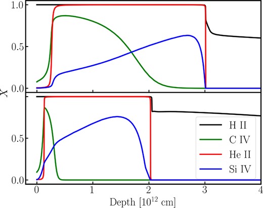
cloudy results of ionization fraction, X, for |$\rm H^{+}$| (black), |$\rm He^{+}$| (red), |$\rm C^{+3}$| (green), and |$\rm Si^{+3}$| (blue), as a function of depth. We use log nH = 10, log ϕ = 19.5, stopping column density |$\log N_{\rm H}=23~\rm cm^{-2}$|, and vturb = 0. For the top panel, Zα = Z⊙, for the bottom panel, Zα = 8Z⊙. As metallicity increases, the volume of the |$\rm C^{+3}$| zone decreases.
Incident and transmitted continuum with the same input parameter as Fig. A1, with Zα = Z⊙. The transmitted continuum is computed using the slab with a cutoff at |$\log d=12.26 \, \rm cm$|.
Essentially, the |$\rm C^{+3}$| ion forms its own Strömgren sphere well inside the outer boundary of the |$\rm He^{+}$| zone. The volume of the |$\rm C^{+3}$| zone is, to a first approximation, determined by the familiar ‘photon counting argument’ (Osterbrock & Ferland 2006). As the metal abundance goes up, the recombination rate per unit volume for |$\rm C^{+3}$| goes up proportionally; and every recombination is balanced by a photoionization that consumes a photon between 3.52 and 4.0 Ryd. Thus, the number of |$\rm C^{+3}$| ions in the slab remains roughy constant. Given that the electron temperature decreases with increasing metallicity, the intensity of the C iv emission line actually decreases as the metal abundance increases. In contrast, the ionization fraction of |$\rm Si^{+3}$| remains nearly constant at log X = −0.75 as metallicity increases. The ionization potential of |$\rm Si^{+2}$| is 2.46 Ryd, so the relatively unabsorbed continuum between 2.5 and 3.5 Ryd is available to maintain the abundance of |$\rm Si^{+3}$|. Therefore, the increasing elemental abundance of silicon gives an increasing intensity of the Si iv emission line.
The straightforward physics behind (Si iv + O iv])/C iv gives confidence in this indicator of metallicity, at least in a qualitative sense. But what factors may affect the calibration of the line ratio in terms of absolute abundances? One issue is the ‘turbulence’ within the BLR. We have mentioned above the importance of this parameter for the Fe ii intensity and other predictions of cloudy models (Sarkar et al. 2021; Temple et al. 2021). The turbulence parameter vturb has some effect on the (Si iv + O iv])/C iv ratio. For our log nH = 10, log ϕ = 19.5 model with solar abundances, this ratio drops from 0.15 for zero turbulence to 0.11 for vturb = 107 cm s−1, then rises slightly to 0.12 for 5 × 107 cm s−1. The effect of this is to increase the metallicity required to reproduce a particular value of (Si iv + O iv])/C iv when vturb ≈ 107 cm s−1, compared to vturb = 0.
The nitrogen abundance has some impact on (Si iv + O iv])/C iv. The ionization potential of |$\rm N^{+2}$| is 3.49 Ryd, nearly the same as for |$\rm N^{+2}$|. Therefore, photoionization of |$\rm N^{+2}$| competes for the same scarce photons between 3.5 and 4.0 Ryd that ionize |$\rm C^{+2}$|. A high abundance of nitrogen will therefore reduce the volume in which |$\rm C^{+3}$| is abundant. To explore this effect, we reran the above model with Z = 4 Z⊙ but with N/O = 4(N/O)⊙ (i.e. ‘secondary’ nitrogen). The increase in nitrogen reduces the intensity of C iv from 7.9 to 5.5, reflecting a decrease of 0.22 dex in the fractional abundance of |$\rm C^{+3}$|. The (Si iv + O iv])/C iv ratio increases from 0.33 to 0.39. This mimics the effect of raising the metallicity from Zα = 4 and 8 Z⊙ for solar N/O. Therefore, a simultaneous determination of the nitrogen abundance will benefit the accuracy of the metallicity derived from the (Si iv + O iv])/C iv ratio. The effect of helium abundance on (Si iv + O iv])/C iv is less significant. In the preceding model, with N/O = 4(N/O)⊙ but with He/H increased to 0.175 rather than 0.10, the (Si iv + O iv])/C iv ratio drops only from 0.39 to 0.36.
In this paper, we have focused on the (Si iv + O iv])/C iv indicator for the abundance of the alpha-elements. Other indicators can give substantially different results for the BLR metallicity. For example, comparison of figs 22 and 29 of Nagao et al. (006b), for the more luminous quasars, gives roughly solar metallicity from C iii]/C iv but nearly 10 Z⊙ from Al iii/C iv and even higher for the N v indicators. However, as noted by Lai et al. (2022), Al iii and N v are more difficult to measure, and C iii] is sensitive to the ionization parameter and to collisional de-excitation. Moreover, many of the line ratios discussed by Nagao et al. (006a) and others use C iv as the denominator. We have argued here that the ionization structure of C iv largely drives the metallicity dependence of these ratios, and therefore they cannot be considered independent.
APPENDIX B: GALACTIC CHEMICAL EVOLUTION VERSUS SEPAD
For the purpose of constraining the SEPAD scenario (Sections 2 and 4.2) with the abundance properties inferred from observations (Section 4.1), we highlight how different physical processes lead to diverse paths of chemical evolution in the AGN environment versus that in the Galaxy.
A. Galactic stars’ (including the Sun) elemental distribution is the byproduct of their chemical evolution with a conventional initial mass function (IMF) and their mass-dependent evolutionary tracks in the Milky Way disc, halo(Venn et al. 2004), and satellite dwarf spheroidal galaxies (Shetrone, Bolte & Stetson 1998; Hill et al. 2019) in the Galatcic halo.
A1. Enrichment of He, α, and Fe abundances. Hydrogen (H) is converted into helium (He) through the p–p chain or the CNO cycle on the main sequence (MS) while α (including C, O, Si, Mg) and some Fe elements are produced through the triple-α and α-chain process during the post main sequence (PostMS) evolution. Nitrogen (N) is a secondary element enhanced through the CNO cycle on the MS without changes in the total C + N + O abundance. High and intermediate-mass stars (≳8 M⊙), detached from their natal molecular clouds, rapidly evolve off (in ≲108 yr) their MS track, release He and CNO-enriched winds during the Wolf–Rayet and PostMS red giant phases, respectively.
A2. The [α/Fe]ratio. Although Mg is produced in these stars’ deep interior during their hydrostatic phase (Weaver, Zimmerman & Woosley 1978; Nomoto & Hashimoto 1988), its ejection is delayed (Choi et al. 2016) until the advanced PostMS or type II supernova (SN ii) phase, accompanied by comparable amounts of Fe and Si and larger masses of C and O (Thielemann, Nomoto & Hashimoto 1996). Since both Zα and ZFe of the ejecta are several times larger than those inferred for zero-age-main-sequence (ZAM) Sun, this feedback process increases these abundances towards the solar values in the initially pristine ISM. Nevertheless, the abundance ratio of ZFe/Zα is below its solar value due to the slightly less efficient production of Fe than α elements in massive stars (Woosley, Heger & Weaver 2002). Less massive (≤8 M⊙) stars take longer (≳108 yr) time to evolve through the MS phase, becoming red giants with N-enriched winds and ultimately white dwarfs. Those compact remnants located in suitable binary systems eventually undergo type Ia supernova (SN ia) explosions, with the ejection of comparable masses of CNO (∼0.2 M⊙) and Si but larger amounts of Fe (∼0.6 M⊙) (Nomoto, Thielemann & Yokoi 1984; Iwamoto et al. 1999).
These diverse yields from SN ia and SN ii are reflected in the differences in [α/Fe] for stars formed in different epochs. Among the Galactic halo population II and disc stars as well as stars in the Local Group dwarf spheroidal galaxies, the observed values of [α/Fe], including [Mg/Fe], are elevated by ∼0.3–0.5 dex (within ∼2σ standard deviation), while both [α/H] and [Fe/H] are down by 2 to 3 dex (Tolstoy, Hill & Tosi 2009) over an age span of several Gyr. This pattern implies that the α elements contained in these stars, in particular, O, are primarily produced by an early generation of massive stars, whereas the Fe-peak elements in later-generation Pop I stars are mostly generated by SN ia from modest-mass (≲8 M⊙) stars that take longer to evolve (Matteucci 2003). Nevertheless, both the observed Pop II abundances and the theoretical yields imply that a value of [Fe/Mg]II (= [Fe/α]II ∼ −0.3), not vastly lower than the solar value can be generated by SN ii alone (Heger & Woosley 2002). In the ramp-up to the solar value of [Fe/H] and [Fe/Mg] (= [Fe/α]) over several Gyr (at cosmic red-shift zγ ≃ 2–3), SN Ia contribute more Fe than do type II supernovae for a population of stars.
- A3. He enrichment. The MS stars convert H into He and some of which is returned to the ISM through WR and PostMS winds as well as SNs, along with the α and Fe byproducts. Galactic chemical evolution models, studies of H ii regions in the Milky Way, and measurements for individual stars in the solar neighbourhood (Carigi & Peimbert 2008; Peimbert et al. 2016; Valerdi et al. 2021) indicate changes in the Galactic He mass-fraction abundance from its values Y0 (∼ 0.245) to its present-day value (Y⊙ ≃ 0.28)where ΔZO, G and ΔZα, G are the average changes in the mass fraction of oxygen and α elements in the Galaxy (≃ ZO, G and ≃ Zα, G their present-day values).(B1)$$\begin{eqnarray} \Delta Y_{\rm G} \simeq 3.3 \Delta Z_{\rm O, G} \simeq 1.8 \Delta Z_{\rm \alpha , G} \end{eqnarray}$$
- A4. Secondary production of N. Primary-generation stars with Zα, G ≲ Z⊙/5 in the Galactic halo and nearby dwarf galaxies have nearly constant ZN, p/ZO, p(∼10−1.6) whereas this ratio steeply increases with Zα, G among the more metal-rich younger stars(Edmunds & Pagel 1978; Henry, Edmunds & Köppen 2000). This difference has been attributed to a transition between the primary/secondary N production in whichfor [α/H]G≶ − 0.7 respectively during the earliest/later phases of Galactic chemical evolution (Arnett 1996; Meynet & Maeder 2002).(B2)$$\begin{eqnarray} [{\rm N/H}]_{\rm p} \simeq [{\rm \alpha /H}]_{\rm p}, \ \ \ [{\rm N/H}]_{\rm s} \simeq 2 [{\rm \alpha /H}]_{\rm s}, \ \ \ \end{eqnarray}$$
B. SEPAD’s stellar populations. They form in or captured by marginally stable AGN discs (Section 2). They continue to grow until they attain an accretion-wind equilibrium with a radial-dependent skewed top-heavy IMF.
B1. Hypothetical long-lasting massive MS stars accrete disc gas, convert H into He through CNO cycle, release He-enriched byproducts, and substantially increases Yd and N/(C + O) without changing Zα and ZFe (Cantiello et al. 2021).
B2. Transition to PostMS evolution require high-degree of He-byproduct recycling (Ali-Deb et al., in preparation). He retention also increases |$\mu_{\star}$| and reduces equilibrium mass by releasing He-byproducts to the disc.
B3. On the PostMS track, He is converted into α elements through triple-α and α-chain reactions and release intense wind with α-enriched byproducts.
B4. Insufficient PostMS pre-collapse mass-loss would lead to the direct collapse and the formation of relatively massive (∼102 M⊙) residual black holes without SN ii. The α and Fe injection into the disc would be largely suppressed. But, if their pre-collapse mass is able to reduce to ∼8–15 M⊙ by strong PostMS winds, these stars would undergo SN ii and release α and Fe-peak ejecta with a sub-solar [Fe/α], and leave behind remnant black holes (with a few M⊙) and neutron stars.
B5. Embedded residual black holes continue to gain mass without heavy-element pollution through gas accretion and merger events which also lead to LIGO/Virgo gravitational wave events.
B6. Neutron stars and white dwarfs may form in the outer region of persistent (≳108 yr) low-luminosity AGN discs around modest SMBH. Merging neutron stars lead to gravitational wave events with copious r-processes byproducts (such as GW170817) and accretion of disc gas onto white dwarfs lead to their collapse with SN ia and super-solar [Fe/α] ejecta.
B7. AGN discs are supplied at their outer radii by metal-deficient gas (with [α/H] and [Fe/H] ≲ 0) from their host galaxies. The injected He, α, and Fe byproducts (at large to small disc radii) are mixed with the turbulent disc gas as it flows inwards (due to viscous stress) towards the SMBH. An asymptotic equilibrium between injection, diffusive mixing, and advection is established with a radial distribution of these elements (Zhou et al., in preparation).
