


ABSTRACT
Gas in the central regions of cool-core clusters and other massive haloes has a short cooling time (≲1 Gyr). Theoretical models predict that this gas is susceptible to multiphase condensation, in which cold gas is expected to condense out of the hot phase if the ratio of the thermal instability growth time-scale (tti) to the free-fall time (tff) is tti/tff ≲ 10. The turbulent mixing time tmix is another important time-scale: if tmix is short enough, the fluctuations are mixed before they can cool. In this study, we perform high-resolution (5122 × 768–10242 × 1536 resolution elements) hydrodynamic simulations of turbulence in a stratified medium, including radiative cooling of the gas. We explore the parameter space of tti/tff and tti/tmix relevant to galaxy and cluster haloes. We also study the effect of the steepness of the entropy profile, the strength of turbulent forcing and the nature of turbulent forcing (natural mixture versus compressive modes) on multiphase gas condensation. We find that larger values of tti/tff or tti/tmix generally imply stability against multiphase gas condensation, whereas larger density fluctuations (e.g. due to compressible turbulence) promote multiphase gas condensation. We propose a new criterion min (tti/min (tmix, tff)) ≲ c2 × exp (c1σs) for when the halo becomes multiphase, where σs denotes the amplitude of logarithmic density fluctuations and c1 ≃ 6, c2 ≃ 1.8 from an empirical fit to our results.
1 INTRODUCTION
Galaxy clusters are the largest gravitationally relaxed objects in the universe. Based on the central temperature/entropy of the gas in their central regions, clusters are broadly divided into two types–cool cores (CC) and non-cool cores (NCC). CC clusters cool radiatively and in the absence of any external heating, they can generate massive cooling flows (100–|$1000~\mathrm{M}_\odot \, \mathrm{yr}^{-1}$|) (Fabian 1994). Such massive cooling flows are not observed in most clusters and the brightest cluster galaxies (BCGs) are rarely star forming. Heating by energy injected from the active galactic nucleus (AGN) is expected to offset the cooling in galaxy clusters – the net mechanical energy input from the AGN, estimated from X-ray cavities roughly balances out the cooling (Fabian 2012; McNamara & Nulsen 2012; Olivares et al. 2022).
While the ICM is expected to be in global thermal balance, localized density perturbations can lead to condensation of cold gas from the hot medium. Filaments of atomic gas (at ∼104 K) and molecular gas (at ∼10 K) are seen ubiquitously, often co-spatial with dense regions in the hotter (107–108 K) X-ray emitting phase (Werner et al. 2013; Anderson & Sunyaev 2018; Olivares et al. 2019). Theoretical studies such as McCourt et al. (2012), Sharma et al. (2012), and Voit et al. (2017) point towards the existence of a critical value of the ratio between the hot gas cooling time (tcool) and the free-fall time (tff), i.e. tcool/tff. If tcool/tff ≲ 10, then seed perturbations in the thermally unstable hot gas lead to the condensation of cold gas. Multiwavelength observations of clusters also show the existence of cold gas in cluster cores around regions where tcool/tff ≲ 10–20 (Voit & Donahue 2015; Lakhchaura et al. 2018; Olivares et al. 2019; O’Sullivan et al. 2021).
Numerical simulations offer us some further insights. Cluster-scale simulations including AGN feedback loop such as Prasad, Sharma & Babul (2015); Beckmann et al. (2019) show that galaxy clusters go through cycles of gas condensation (when |$t_{\mathrm{cool}/t_{\mathrm{ff}}}\lesssim 10$|). Mass accretion on to the central supermassive black hole (SMBH), which releases jets that heat the ICM, raises the value of tcool/tff to prevent further condensation. Once the heating stops due to a lack of mass accretion, cooling takes over and this cycle repeats.
However, there are some challenges to these models. Choudhury, Sharma & Quataert (2019) show that the threshold for cluster atmospheres to be thermally stable increases with increasing amplitude of seed density fluctuations. Nelson et al. (2020) study the formation of small-scale cold gas in the circumgalactic medium (CGM) of galaxies in the TNG50 simulations. They find that cold clouds form due to large (order unity) perturbations in the gas density, which can trigger multiphase condensation in haloes with tcool/tff > 10. Choudhury et al. (2019) show that the threshold condition for multiphase condensation applies to the local value of tcool/tff, rather than its globally averaged value. On a similar note, Voit (2021) proposes that locally tcool/tff ≲ 1 leads to condensation but on a global scale the threshold condition depends on the amplitude of entropy fluctuations.
Turbulence plays a critical role in the evolution of the ICM. It is driven on large scales (∼100–500 kpc) by galaxy motions during mergers and on smaller scales by AGN (∼10–100 kpc). It can transfer the heat from the gas heated by AGN jets to the ambient ICM through turbulent mixing (Banerjee & Sharma 2014) and viscous dissipation. Further, Voit (2018) shows that turbulence can drive buoyancy oscillations that lead to condensation when 10 ≲ tcool/tff ≲ 20. Gaspari et al. (2018) argue that the turbulent mixing time tmix is a more important time-scale than tff, and the regions with cold gas are traced better by tcool/tmix ≲ 1. Mohapatra & Sharma (2019) show that the onset of multiphase condensation is delayed when one drives turbulence on smaller scales, since tmix is shorter for small-scale driving.
Olivares et al. (2019) and O’Sullivan et al. (2021) find that tcool/tmix ≈ 1 in regions of clusters, where the cold-phase gas is observed. However, it is difficult to disentangle the importance of the two ratios (tcool/tff) and tcool/tmix) from observations, since (1) tcool varies more strongly with radius compared to tff and tmix in cluster centres, and (2) we do not have many direct observations of turbulent velocities of the hot phase, except by Hitomi for the Perseus cluster (Hitomi Collaboration 2016). Hence, we rely on indirect methods of constraining turbulence and tmix (see Simionescu et al. 2019 for a review).
Turbulence plays a dual role in multiphase condensation. On one hand, turbulence drives large density fluctuations on the driving scale in the ICM, leading to multiphase gas condensation. On the other hand, turbulent mixing suppresses the density contrast and multiphase condensation. Baek et al. (2022) find molecular gas co-spatial with sloshing features seen in the X-ray emission, implying that the velocity field affects condensation locally. Using idealized simulations, Mohapatra, Federrath & Sharma (2020, 2021, 2022b) have shown that the amplitude of turbulence-driven (other sources, e.g. cooling, buoyancy, jet/outflows can also drive density fluctuations) density fluctuations depends on the degree of stratification of the ICM, the turbulent Mach number and the nature of driving (solenoidal versus compressive modes). However, many previous theoretical and numerical studies of the ICM initialize seed density fluctuations by hand, independent of the gas turbulence.
In order to better constrain the conditions required for the onset of multiphase condensation and to separate the two proposed threshold ratios of the time-scales, we conduct high-resolution hydrodynamic simulations of turbulence in a stratified medium, including radiative cooling of the gas. In our study, density fluctuations develop naturally due to the large-scale turbulence driving. We vary four main parameters relevant to cluster haloes – (1) the strength of stratification, which controls tff, (2) the strength and (3) the nature of turbulence forcing, which controls tmix and the amplitude of density fluctuations, and (4) the initial gas density, which controls tcool.
This paper is organized as follows. We introduce our model, numerical set-up and tools in Section 2. Then we present our results and discuss them in the context of galaxy cluster haloes in Section 3. We summarize our key findings regarding the two time-scale ratios in Section 4. In Section 5, we discuss some of the shortcomings of our model and set-up, missing physics and how they might affect our results as well as the future prospects of this work. Finally, we present our concluding remarks in Section 6.
2 METHODS
2.1 Model equations
We use Euler equations to model the ICM, with acceleration due to gravity (|$\boldsymbol {g}$|) and turbulence (|$\boldsymbol {a}$|), radiative cooling with a rate density |$\mathcal {L}$|, and thermal heating with a rate density Q as additional source terms. We assume an ideal gas equation of state with an adiabatic index γ = 5/3. We evolve the following equations:
where ρ is the gas mass density, |$\boldsymbol {v}$| is the velocity, P = ρkBT/(μmp) is the thermal pressure, μ is the mean particle weight, mp is the proton mass, kB is the Boltzmann constant, and T is the temperature. In the energy equation (equation 1c), the total energy density is given by E and the cooling rate density |$\mathcal {L}$| is given by
where ne and ni are the electron and ion number densities, respectively. We use the temperature-dependent cooling function Λ(T).
2.2 Important time-scales
The time-scales of interest in this study are – the gas cooling time tcool, the isobaric thermal instability growth time tti, the sound crossing time tcs, the gas free-fall time tff and the turbulent mixing time on the driving scale tmix. They are defined as follows:
where α characterizes the density dependence of the heating rate density Q, with Q ∝ ρα. The sound speed cs is given by |$\sqrt{\gamma P/\rho }$|. For a derivation of equation (3b) using linear stability analysis, see section 4.1 in McCourt et al. (2012). The two scales L and ℓdriv denote the size of the system and the driving scale of turbulence, respectively. In our simulations, ℓdriv = L/2 and |$v_{\ell _{\mathrm{driv}}}\approx v$|, so tmix ≃ L/(2v).
2.3 Numerical methods
We use a modified version of the flash code (Fryxell et al. 2000; Dubey et al. 2008), version 4, to solve equation (1a) to equation (1d) in our simulations. For time integration, we use the MUSCL-Hancock scheme (Van Leer 1984; Waagan 2009) with the HLL5R approximate Riemann scheme (Waagan, Federrath & Klingenberg 2011). We use a second-order reconstruction method that uses primitive variables and ensures that density and internal energy are positive. Our simulation domain size is the same as in Mohapatra et al. (2020) – we use a cuboidal box with Lx = Ly = L = 40 kpc and Lz = 1.5L = 60 kpc. The box is centred at the origin (0,0,0). We implement periodic boundary conditions along the x- and y-direction for all variables. In the z-direction, we implement diode boundary conditions for the velocity. For density and pressure, we fix the values in the guard cells to their initial values throughout the duration of the simulation. In addition to using a larger box along the z direction to minimize the effect of the boundaries, we further smoothly decay the source terms – turbulent acceleration |$\boldsymbol {a}$|, gas cooling rate density |$\mathcal {L}$|, and gas heating rate Q for |z| > L/2, where the weighting function w(z) is given by
We analyse the outputs from our simulations only in the central cubical region with |x|, |y|, |z| < L/2.
2.4 Problem set-up
2.4.1 Initial density and pressure profiles
We set-up a gravitationally stratified atmosphere with a constant |$\boldsymbol {g}$| oriented along the |$-\hat{\boldsymbol {z}}$| direction. Pressure and density follow exponential profiles along the z direction at time t = 0 and the gas is at hydrostatic equilibrium, given by
H is the scale height of pressure/density and P0, ρ0 (=P0/gH) are the initial values of pressure and density at z = 0, respectively. The pseudo-entropy S = P/ργ has a scale height HS(≡ 1/[dln S/dz]) = H/(γ − 1). Since γ = 5/3, HS > 0, and the equilibrium is convectively stable. The degree of stratification is denoted by the Froude number Fr on the integral scale ℓint and is given by
and |$N=\sqrt{g/(\gamma H_S)}$| is the Brunt–Väisälä oscillation frequency, and v is the rms velocity. The quantity E(k) denotes the velocity power spectrum.
2.4.2 Turbulent forcing
To force turbulence, we use a spectral forcing method using the stochastic Ornstein–Uhlenbeck (OU) process to model |$\boldsymbol {a}$| (Eswaran & Pope 1988; Schmidt, Hillebrandt & Niemeyer 2006; Federrath et al. 2010).1 The autocorrelation time of the driving is set to roughly match an eddy turnover time on the driving scale. We drive turbulence only on large scales, corresponding to 1 ≤ k|L/2π ≤ 3, where k is the magnitude of the wave vector |$\boldsymbol {k}$|. The power is a parabolic function of k, peaking at 4π/L, which corresponds to ℓdriv = L/2. We consider two types of forcing in this study: (1) natural mixture and (2) compressive modes only. For a more detailed description of the turbulence driving, we refer the reader to section 2.2.1 of Mohapatra, Federrath & Sharma (2022b).
2.4.3 Cooling function
We use the temperature-dependent cooling function from Sutherland & Dopita (1993) corresponding to Z⊙/3 (a third solar) metallicity. To control the code evolution time-step set by tcool, we introduce cut-offs on the cooling rate based on the gas pressure (Pcut-off) and temperature (TCut-off). We switch off the gas cooling when the gas pressure or temperature drop below these cut-off values. We also set a ceiling on the gas density (ρceiling) above which we switch off the cooling. The complete cooling function is given by
where |$\mathcal {H}$| is the Heaviside function. We have set Tcut-off = 104 K, which is also the lower limit of the cooling function in Sutherland & Dopita (1993). We fix Pcut-off = P0/1000 and the ρceiling = 500 × ρ0. For faster time-steps, we modify the criterion for setting the global time-step of the code dtcode, such that dtcode = min(0.5 × subfactor × tcool, min, dtCFL), where tcool, min is the minimum cooling time over the domain, dtCFL is the code time-step set by the Courant–Friedrichs–Lewy criterion and subfactor is the subcycling factor which we set to 25. We refer the reader to appendix C of Mohapatra et al. (2022b) for a discussion of this implementation. Note that we resolve cooling at most times when we update the internal energy using subcycling.
2.4.4 Thermal heating rate and shell-by-shell energy balance
To prevent a runaway cooling flow in the simulation, we implement a shell-by shell balance (in constant z shells) between the net energy lost due to cooling and the net energy added by turbulence and thermal energy input. We inject thermal energy into each shell at a rate Q(z) proportional to the local gas density in each shell (Q ∝ ρ in equation 1c and α = 1 in equation 3b). However, if the turbulent energy input exceeds the total energy lost in a shell due to cooling, we set Q(z) = 0 and do not apply any additional cooling. We implement this energy balance at each time-step. Mathematically, the heating rate is given by
We define the turbulent heating fraction fturb as
where we carry out the volume integration over the region defined by |x|, |y|, |z| < L/2.
2.5 Initial conditions
We set our initial conditions to model the dense central regions of CC clusters. We initialize the gas with a constant initial temperature throughout the domain, set to T0 = 1.07 × 10⁷ K, such that the initial sound speed |$c_{s0}=500~\mathrm{km\, s^{-1}}$|. We set the gas number density |$n_0=0.1\, \mathrm{cm}^{-3}$|, so ρ(t = 0) = n0μmp exp (− z/H) (except for four low-density simulations, where n0 is 2 times smaller). We drive turbulence on 20 kpc scales, which roughly mimics the size of X-ray cavities seen in the ICM (see e.g. Hlavacek-Larrondo et al. 2012, for cavity sizes in the MACS clusters sample). Once turbulence reaches a steady state, the rms velocity of the gas is approximately |$250~\mathrm{km\, s^{-1}}$| for our fiducial runs, consistent with the observations by Hitomi in the core regions of the Perseus cluster (Hitomi Collaboration 2016).
The cooling function Λ(T) ∝ T1/2 for free–free cooling at T ∼ 107K. Since Q ∝ ρ, this gives |$t_{\mathrm{ti}}\approx (10/3)t_{\mathrm{\mathrm{cool}}}$|, using γ = 5/3 in equation (3b).
2.6 List of simulations
We have conducted a total of 16 simulations in this study, which are listed in Table 1. By default, our simulations have 5122 × 768 resolution elements, with 768 cells along the z-axis. Since Lz = 1.5L, the individual resolution elements (or cells) are all cubical, organized in a uniformly spaced Cartesian grid. Since we only use the central cubical region with |x|, |y|, |z| < L/2 for the post-processing of our results, the effective resolution is 5123.
Simulation parameters and volume-averaged quantities for different runs.
| Label | Driving | Fr | tmp (Gyr) | |$\mathcal {M}$| | |$\mathcal {M}_{\mathrm{comp}}$| | |$v\ (\mathrm{km\, s^{-1}})$| | tti/tff | tti/tmix | |$\sigma _{s,\mathrm{hot}}^2$| |
|---|---|---|---|---|---|---|---|---|---|
| (1) | (2) | (3) | (4) | (5) | (6) | (7) | (8) | (9) | (10) |
| H1.0 | Natural | 2.2 ± 0.2 | 1.22 | 0.64 ± 0.01 | 0.13 ± 0.03 | 255 ± 4 | 3.87 ± 0.05 | 5.92 ± 0.08 | 0.029 ± 0.002 |
| H4.0 | Natural | 5.0 ± 0.5 | NA | 0.64 ± 0.01 | 0.12 ± 0.04 | 259 ± 4 | 2.19 ± 0.02 | 6.92 ± 0.04 | 0.023 ± 0.002 |
| ζ0.0H1.0 | Compressive | 0.6 ± 0.1 | 0.24 | 0.40 ± 0.01 | 0.27 ± 0.09 | 172 ± 7 | 6.5 ± 0.2 | 6.2 ± 0.5 | 0.155 ± 0.001 |
| ζ0.0H4.0 | Compressive | 1.6 ± 0.1 | 0.28 | 0.40 ± 0.01 | 0.3 ± 0.1 | 167 ± 6 | 2.9 ± 0.1 | 5.4 ± 0.4 | 0.136 ± 0.005 |
| H1.0wdriv | Natural | 0.20 ± 0.01 | NA | 0.076 ± 0.001 | 0.015 ± 0.004 | 39 ± 1 | 6.2 ± 0.1 | 1.43 ± 0.05 | 0.006 ± 0.001 |
| H4.0wdriv | Natural | 0.31 ± 0.02 | 1.32 | 0.047 ± 0.004 | 0.005 ± 0.001 | 24 ± 3 | 2.77 ± 0.06 | 0.8 ± 0.1 | 0.012 ± 0.005 |
| H1.0sdriv | Natural | 2.1 ± 0.2 | 0.19 | 0.94 ± 0.02 | 0.24 ± 0.05 | 385 ± 1 | 4.0 ± 0.1 | 9.3 ± 0.2 | 0.10 ± 0.02 |
| H4.0sdriv | Natural | 11.0 ± 1.0 | NA | 0.59 ± 0.03 | 0.11 ± 0.04 | 410 ± 20 | 7.1 ± 0.1 | 35.0 ± 2.0 | 0.017 ± 0.001 |
| H1.0ldens | Natural | 2.5 ± 0.1 | NA | 0.72 ± 0.04 | 0.14 ± 0.03 | 270 ± 10 | 6.6 ± 0.2 | 10.4 ± 0.1 | 0.038 ± 0.004 |
| H4.0ldens | Natural | 5.5 ± 0.9 | NA | 0.65 ± 0.02 | 0.12 ± 0.03 | 266 ± 8 | 4.52 ± 0.06 | 14.6 ± 0.2 | 0.022 ± 0.002 |
| ζ0.0H1.0ldens | Compressive | 1.2 ± 0.09 | 0.47 | 0.49 ± 0.05 | 0.29 ± 0.08 | 210 ± 20 | 13.5 ± 0.6 | 16 ± 3 | 0.18 ± 0.06 |
| ζ0.0H4.0ldens | Compressive | 3.0 ± 0.4 | 0.47 | 0.49 ± 0.03 | 0.29 ± 0.08 | 210 ± 20 | 6.4 ± 0.3 | 16 ± 2 | 0.17 ± 0.04 |
| H1.0NoTurb | NA | 0.33 ± 0.03 | NA | 0.10 ± 0.01 | 0.019 ± 0.004 | 52 ± 1 | 6.63 ± 0.03 | 2.07 ± 0.06 | 0.007 ± 0.001 |
| H4.0NoTurb | NA | 0.36 ± 0.05 | 0.52 | 0.05 ± 0.01 | 0.013 ± 0.009 | 23 ± 4 | 2.80 ± 0.04 | 0.8 ± 0.2 | 0.013 ± 0.003 |
| H1.0HR | Natural | 2.2 ± 0.1 | 1.45 | 0.70 ± 0.02 | 0.15 ± 0.05 | 266 ± 6 | 3.6 ± 0.1 | 5.9 ± 0.1 | 0.043 ± 0.003 |
| H4.0HR | Natural | 4.8 ± 0.1 | NA | 0.66 ± 0.02 | 0.12 ± 0.03 | 261 ± 7 | 2.19 ± 0.03 | 7.03 ± 0.08 | 0.025 ± 0.003 |
Note. Column 1 shows the simulation label. The number following H denotes the scale height of the initial pressure/density profile in code-units. We show the type of turbulence driving in column 2. In column 3, we show the average Froude number Fr of the simulations. The fourth column shows the time at which multiphase gas condenses out of the hot phase through thermal instability for a simulation. We denote it as ‘NA’ if there is no multiphase gas condensation in the particular simulation. In columns 5 and 6, we show the volume-weighted rms Mach number and its compressive component |$\mathcal {M}_\mathrm{comp}$|, respectively. In column 7, we show the volume-weighted standard deviations of velocity v. We show the average value of the ratio between the thermal instability time-scale tti and important dynamical time-scales – the free-fall time-scale tff and the turbulent mixing time-scale tmix in columns 8 and 9, respectively. Finally, in column 10, we show |$\sigma ^2_{s,\mathrm{hot}}$|, the square of the standard deviations of the logarithms of density of the hot phase. All time-averaged statistics in columns 3, 5, 6, 7, 8, 9, and 10 are averaged for t ≤ tmp for runs in which multiphase gas forms. Movies of simulations are available at this playlist.
By default, we drive the natural mixture of turbulent modes (i.e. we do not remove either solenoidal or compressive components of |$\boldsymbol {a}$|; see Federrath et al. 2010). Our fiducial set consists of two simulations with different strengths of gravity/stratification (and different tff) labelled H1.0 and H4.0 (so the value of g is in the ratio 4:1). The number following H in the label denotes the scale height of pressure/density in the simulation in code units (i.e. with respect to L). We repeat this fiducial set as we vary other simulation parameters in our set. To check the effect of the nature of turbulence forcing, we keep all other parameters fixed but set |${\boldsymbol \nabla \times } {\boldsymbol {a}}=\boldsymbol {0}$| (compressive forcing; see Federrath et al. 2010). These two runs are indicated by ζ0.0 in the label, where ζ denotes the fraction of solenoidal modes. In order to vary tmix while keeping tti and tff constant, we have two sets of simulations with weak driving and strong driving, denoted as ‘wdriv’ and ‘sdriv’ in the labels, respectively. Similarly, to check the effect of a longer tti, we repeat the fiducial set and compressive forcing set of simulations with half the initial density (n0 = 0.05 cm−3) and pressure, so that the initial temperature still stays the same. This doubles the initial tti and tcool. These four runs are marked by ‘ldens’ (low density) in the label. To compare our results directly with previous studies without constant turbulent forcing, we switch off the turbulent forcing and repeat the fiducial set with seed density perturbations at t = 0. These are marked by ‘NoTurb’ in the run label. Finally, to check the convergence of our results, we have two higher resolution versions of our fiducial simulations with 10242 × 1536 resolution elements. These simulations are denoted by ‘HR’ in the label.
3 RESULTS AND DISCUSSION
In this section, we present and discuss the results of our simulations. We have run all our simulations till tend = 2.344 Gyr. Thermal instability leads to cold gas condensing out of the hot phase in 8 out of our 14 simulations. For runs that form multiphase gas, we define the time at which cold (T ≲ 2 × 10⁴ K) gas first forms (when the cold gas mass fraction |$m_{\mathrm{cold}}/m_{\mathrm{tot}}\gt 0.01~{{\ \rm per\ cent}}$|) as tmp and list it in column 4 of Table 1. We have also listed some time and volume-averaged statistics in Table 1, such as Fr, the rms Mach number |$\mathcal {M}$|, the rms velocity v, the average value of the ratio between important time-scales tti/tff and tti/tmix, and the square of logarithmic-density (s) fluctuations |$\sigma _{s,\mathrm{hot}}^2$| in columns 3, 5, 6, 7, 8, and 9, respectively. For runs that do not form multiphase gas, these quantities are averaged over the last 120 Myr of the simulation. For runs that form multiphase gas, these averages are calculated in the 120 Myr just before tmp, but after the first 100 Myr, so that there is some time for turbulence to grow.2
We begin this section by briefly discussing some key statistical properties of the gas in the fiducial set and the compressive forcing set of runs. These are crucial to understanding the second part of our study, where we vary the simulation parameters such as the strength of the turbulence forcing and the cooling rate. In the later subsections, we move our focus to the non-linear evolution of thermal instability in the system and how it is affected by the different parameter choices.
3.1 Fiducial and compressive forcing runs
3.1.1 Projection maps perpendicular to the stratification
Three of these runs form cold gas through thermal instability, but the H4.0 run does not. In Fig. 1, we show the projections of gas density (volume-weighted, first column), temperature (mass-weighted, second column), and column density fluctuations (after dividing out the xy-averaged density profile) in the hot phase (T ≥ 106 K, third column). These snapshots are plotted when the runs have the maximum mass fraction of cold gas (mcold/mtot) and at t = tend for the H4.0 run. The insets in column 1 show the projections of gas density at t = 0. Clearly, the runs with H = 1.0 have stronger gradients in the initial density than the runs with H = 4.0.
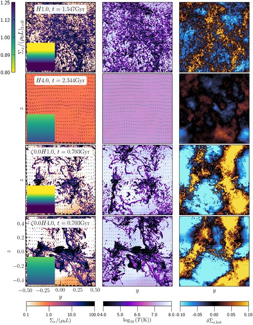
Density (volume-weighted), temperature (mass-weighted), and normalized column density fluctuations in the hot phase (T > 106 K), integrated along the x-axis for our fiducial and compressive driving sets of runs. The insets in column 1 show the column density of the gas at t = 0. Cold gas forms through condensation from the hot phase for all runs except the H4.0 run. This produces large variations in the gas density and temperature. The compressive forcing runs produce large-scale cold filamentary clouds.
Thermal instability produces large variations in density, with much stronger variations compared to the initial density gradient. In all runs that form multiphase gas, the dense regions correspond to cooler gas and the rarer regions correspond to hotter gas, as expected. For the H1.0 run, the cold clouds are misty, i.e. they are small in size and occur throughout the simulation domain. In comparison, the compressive driving runs show many large clouds, with size ∼ℓdriv = 20 kpc. These results are similar to what we observed for different forcing runs in simulations without gravity in Mohapatra et al. (2022b).
For the H4.0 run, the net variations in density and temperature are much smaller compared to the other runs. Column density fluctuations in the hot phase are also much weaker for this run. For the other runs, we find that the regions with cold gas (in column 2) are associated with strong, positive fluctuations in the column density in the hot phase (in column 3). Such features are also observed in multiwavelength observations of the ICM (see e.g. Werner et al. 2013; Anderson & Sunyaev 2018; Baek et al. 2022). In our simulations, the spatial overlap between the different phases could be either due to turbulent mixing with the cooler gas making the hot phase denser or the cold gas could have directly formed from these dense regions of the hot gas, which have shorter cooling time (since tcool ∝ ρ−1).
3.1.2 Time-evolution of volume-averaged quantities
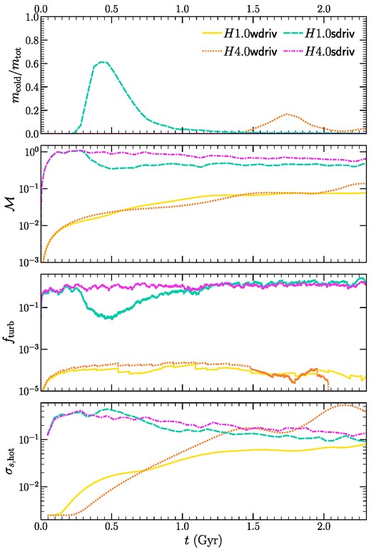
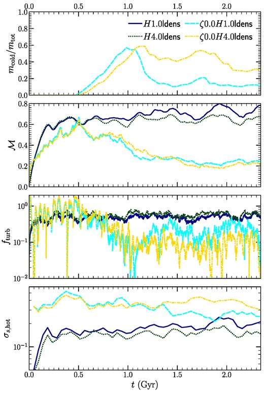
In Fig. 2, we show the time evolution of the mass fraction of cold gas (T ≲ 2 × 10⁴ K) in the first row, the volume-averaged |$\mathcal {M}$| in the second row, fturb (defined in equation 6c) in the third row and the standard deviation of logarithmic density of the hot-phase σs, hot in the fourth row.
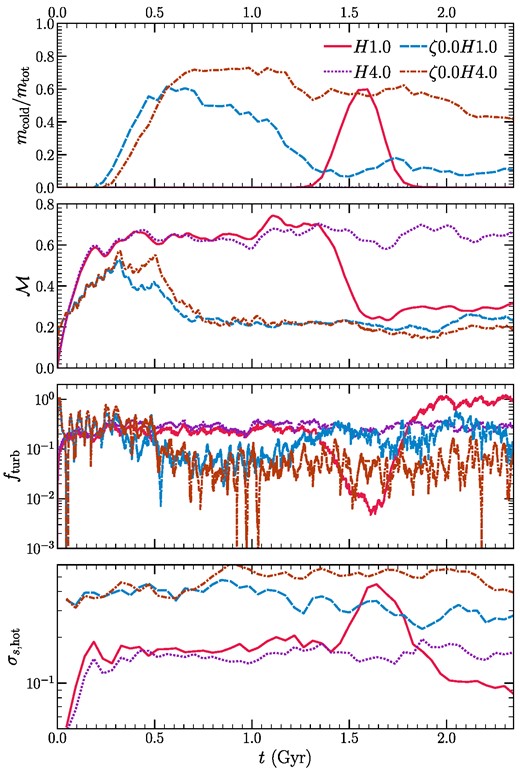
Time evolution of the cold-gas mass fraction (first row), volume-weighted rms Mach number (second row), turbulent heating fraction fturb (third row), and amplitude of logarithmic density fluctuations in the hot phase (T > 106 K, fourth row), for our fiducial and compressive driving sets of runs.
Cold gas forms at different times (tmp) for the three different runs. The time tmp is clearly affected by the driving, multiphase gas condensation occurs much earlier for the compressive forcing runs. This is due to the stronger seed density fluctuations generated by the compressive forcing, as seen in the fourth row of Fig. 2. The ratio mcold/mtot initially increases, reaches a maximum value, and then decreases with time. The rate of decrease in mcold/mtot is much faster for the runs with stronger gravity (i.e. H = 1.0), since the cold clumps being heavier than the ambient hot gas, fall faster to the negative z boundary.
At initial times, |$\mathcal {M}$| for all runs reaches values of 0.5–0.7. The turbulent heating fraction fturb is approximately a few |$\times \,\,10~{{\ \rm per\ cent}}$|. However, for the runs forming multiphase gas, we find that both |$\mathcal {M}$| and fturb decrease at t = tmp. By design, the turbulent forcing amplitude remains the same throughout the duration of the simulation. Cold-gas condensation is associated with the production of fast-cooling dense gas at intermediate temperatures (2 × 10⁴ K ≲ T ≲ 106 K), which increases the cooling rate. This is compensated by an increase in the heating rate since we impose energy balance in z-shells. The rarer hot-phase gas is heated more (because |$\mathcal {L}\propto \rho ^2$|, Q ∝ ρ), which increases cs and decreases |$\mathcal {M}$|.
At late times, the simulation reaches a steady state at a lower |$\mathcal {M}$| but higher fturb. The atmosphere is hotter and has a smaller net cooling rate, such that fturb increases. For the H1.0 run, after the removal of extra mass, the turbulent heating alone is sufficient to balance the reduced steady-state cooling rate (fturb = 1).
Among the two fiducial runs (H1.0 and H4.0), the hot-gas density fluctuations are slightly larger for the H1.0 run for t < tmp. This happens because the H1.0 run is more strongly stratified (Fr listed in column 3 of Table 1) compared to the H4.0 run. Mohapatra et al. (2020, 2021) showed that for weak and moderate levels of stratification (Fr ≳ 1) the density fluctuations increase with increasing stratification (decreasing Fr) for fixed |$\mathcal {M}$| and driving. These larger seeds lead to multiphase condensation developing in the H1.0 run (and a slightly shorter cooling time, whose effect we discuss later), whereas they do not develop in the H4.0 run.
The hot-gas density fluctuations show a sharp increase at t ≳ tmp for the H1.0 run – bringing its value closer to the amplitudes for the compressive forcing runs. Clearly, the density fluctuations due to multiphase condensation are much larger than those due to stratified turbulence at t < tmp. Using unstratified multiphase turbulence simulations in Mohapatra et al. (2022b, fig. 6 and section 3.5), we showed that these larger fluctuations are due to the strong compressive velocities during cold-gas condensation and the baroclinicity of a multiphase turbulent system.
3.1.3 Mach number, temperature, and density distributions
In Fig. 3, we show the mass-weighted probability distribution functions (PDFs) of the Mach number (first column), temperature (second column), and gas density (third column) for our fiducial and compressive driving sets of runs. The PDFs for the three multiphase runs are averaged from 1.4 to 1.64 Gyr and for the single-phase H4.0 run, they are averaged from 1.4 Gyr till tend. We show the 1 − σ spread in PDF values as shaded regions. The runs forming multiphase gas show two strong peaks in all three PDFs, whereas the H4.0 run shows a single peak. The two peaks correspond to the hot and cold phases.
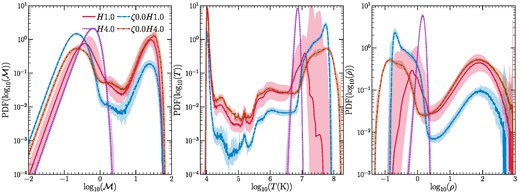
The mass-weighted PDFs of Mach number (left), temperature (middle), and density (right), for our fiducial and compressive driving sets of runs. The H4.0 run does not form cold gas and shows a single peak in all distributions, while the other three runs that form cold gas show two strong peaks, corresponding to the hot and cold phases. The hot-phase gas is hotter (by about an order of magnitude) for the two compressive forcing runs.
The hot phase is subsonic (|$\mathcal {M}_{\mathrm{hot}}\lt 1$|) for all four runs, as is expected from ICM observations (Hitomi Collaboration 2016, see Simionescu et al. 2019 for a review). The high |$\mathcal {M}$| peak corresponds to the supersonic cold-phase gas, which has much smaller sound speed. Since we use the same forcing scheme to drive turbulence in all four runs, the shapes of the distributions of |$\mathcal {M}$| are quite similar for |$\mathcal {M}\lesssim 1$|. The small offsets can be explained by differences in the temperature/sound speed among the different runs.
In the temperature PDFs, we observe a strong cold-phase peak at Tcut-off = 104 K and the hot-phase peak at T ∼ 107–108 K. The features in the PDF between these two peaks correspond to the shape of the cooling curve that we use. The temperature of the hot-phase peak is higher for the compressive forcing runs.
In the density PDFs, the low-density peak corresponds to the hot phase and the high-density peak to the cold phase. The hot-phase gas has much lower density for the compressive forcing runs, while the density of the cold-phase peak is similar. Thus, the ratio between the densities of the phases χ = ρcold/ρhot is much larger for compressive forcing. This is caused by strong converging and diverging motions on the driving scale (Schmidt et al. 2009; Federrath et al. 2010; Seta & Federrath 2022). For the H4.0 run, the density PDF is lognormal with a power-law tail at low densities. The low-density tail is a known feature of the PDFs when the adiabatic index γ > 1, also reported in Passot & Vázquez-Semadeni (1998), Federrath & Banerjee (2015), and Mohapatra et al. (2020).
3.1.4 Density–temperature phase diagram
In Fig. 4, we show the joint mass-weighted PDFs of the logarithms of temperature and density, temporally averaged over the same duration as the 1D PDFs in Fig. 3. The different lines show the nature of fluctuations: adiabatic (δT/T0 ∝ (γ − 1)δρ/ρ0), isothermal (δT = 0) at 105.5 K and Tcut-off = 104 K, isobaric (δT/T0 = −δρ/ρ0), and isochoric (δρ/ρ0). From a theoretical viewpoint, understanding the nature of fluctuations is important to calculate the growth rate of thermal instability through the different fluctuation modes (Das, Choudhury & Sharma 2021). They are also useful to compare with observations. For instance, Zhuravleva et al. (2018) inferred the mode of perturbations from X-ray observations of the ICM.
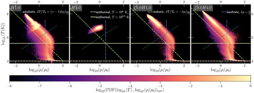
The mass-weighted 2D PDFs of T versus ρ for our fiducial and compressive driving sets of runs. The single-phase H4.0 run shows a mixture of isobaric and adiabatic modes. The three multiphase runs show an isobaric hot phase (T > 106 K), an isochoric intermediate phase (2 × 10⁴ K < T < 106 K), and an isothermal cold phase (T ≲ 2 × 10⁴ K).
In our single-phase H4.0 run, the fluctuations are composed of isobaric and adiabatic components. This is in agreement with the stratified turbulence simulations (without radiative cooling) of Mohapatra et al. (2020), where we showed that unstratified turbulence produces adiabatic fluctuations, and the fraction of isobaric fluctuations increases with increasing strength of the stratification.
For the multiphase runs, we observe some clear trends in the PDFs – the hot phase (106–108 K) is isobaric, the intermediate temperatures are isochoric, with a drop in temperature around 105.5–106 K and the cold phase is approximately isothermal at Tcut-off. We reported the same features in the temperature–density joint PDFs in Mohapatra et al. (2022b, fig. 5), so they are not strongly affected by the stratification.
The isochoric drop at T ∼ 105.5–106 K is associated with the peak of Λ(T), where tcool < tcs. The cooling time for the gas at intermediate temperatures is quite short and such gas may not be able to attain pressure equilibrium. However, some of this pressure drop could be due to our lack of resolution of the cooling length (ℓcool = min (cstcool)). Recent high-resolution simulations of multiphase systems such as Fielding et al. (2020); Abruzzo, Fielding & Bryan (2022) argue that this could be due to lower spatial resolution in large-scale boxes, which do not resolve ℓcool. While resolving ℓcool is important to model the properties of the cold phase after it forms, it is not necessary to determine when or where it forms. In this study, we mainly focus on the latter part, so we do not expect our results to strongly depend on resolution. We have checked our results for convergence in the Appendix. The TNG50 simulations (Nelson et al. 2020; Ramesh, Nelson & Pillepich 2023), which track the cold gas better than our fixed-grid simulations, do not show this isochoric drop. However, this could be partly due to the orders of magnitude variation in halo pressure in TNG50 haloes (therefore the sharp isochoric temperature drop is not as clear), whereas the vertical extent of our simulation box is much smaller to have a large pressure variation.
3.1.5 Evolution of the z-profile of entropy
Theoretical studies such as Voit et al. (2017) report that the large-scale entropy gradient is important to thermal instability. They propose that haloes in thermal balance (applicable to our set-up) with a shallower entropy gradient are more susceptible to condensation. In Fig. 5, we show the z-shell averaged entropy profiles ([S/S0](z), where |$S_0=P_0/\rho _0^\gamma$|) of the hot gas (T ≳ 106 K) for our fiducial and compressive forcing sets of runs at t = 0 and t = tend. For the three runs that form multiphase gas, we also plot the entropy profile at the onset of multiphase condensation (tmp, denoted in the titles of the respective columns).
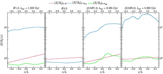
The vertical profiles of entropy of the hot phase (T ≳ 106 K, averaged along the x–y plane) at t = 0 (red dotted line) and t = tend (blue dash–dotted line) for our fiducial and compressive driving sets of runs. We also show the entropy profile at t = tmp (green dashed line, when cold gas has just started forming) for runs that form multiphase gas.
For the H1.0 run, the entropy gradient is steep at t = 0, but it flattens out around the onset of multiphase condensation (t = tmp). This is due to turbulent mixing, which mixes the low- and high-entropy regions together and makes the entropy gradient disappear. After cold gas condenses and moves out of the box through the bottom z boundary, at t = tend the entropy increases by almost an order of magnitude. We find that the gas has redeveloped a weak entropy gradient at this time.
The single-phase H4.0 run starts out with a much weaker entropy gradient compared to the H1.0 run. Despite starting out with a flatter entropy gradient, this run never forms multiphase gas. By t = tend, its entropy gradient also disappears and its entropy value is slightly larger than that for the H1.0 run just before condensation.
The two compressive forcing runs form multiphase gas fairly quickly. Our snapshots just before thermal condensation show that the initial entropy profiles have large-scale variations even within the first ∼300 Myr of the simulations. By this time, the turbulence is still developing, such that a large-scale entropy gradient has not been lost to the mixing. By t = tend, the average entropy for both runs increases by an order of magnitude. Unlike the H1.0 run, we still observe a strong entropy gradient for the ζ0.0H1.0 run. The large-scale entropy profile shows a very disturbed state for the ζ0.0H4.0 run due to strong large-scale perturbations induced by the compressive forcing, which are not moved out of the box by the weaker gravity.
In summary, we find that a smaller initial entropy gradient (larger H) does not necessarily imply better thermal stability of the halo. The entropy profile can be strongly modified by large-scale turbulence, which can remove the initial gradients, given enough time (H1.0 and H4.0 runs). Further, the different amplitudes of density fluctuations also play a key role – larger fluctuations can seed multiphase condensation even when the entropy gradient is steep.
3.1.6 Evolution of z-profiles of important time-scales
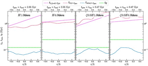
Following the discussion on the role played by the entropy profile, we now move our attention to the z shell-averaged values of the three important time-scales of the system tti, tmix, and tff (defined in Section 2.2). The ratio between these time-scales is expected to play a key role in the thermal stability of the system and has been studied in theoretical (e.g. McCourt et al. 2012; Sharma et al. 2012; Gaspari et al. 2018), numerical (e.g. Prasad et al. 2015; Beckmann et al. 2019; Butsky et al. 2020), and observational (e.g. Voit & Donahue 2015; Olivares et al. 2019) studies. In Fig. 6, we show these quantities for the hot phase (T ≥ 106 K) at t = 0 and at the onset of multiphase condensation (tplot = tmp). For the runs that do not form multiphase gas, we set tplot = tend = 2.344 Gyr.
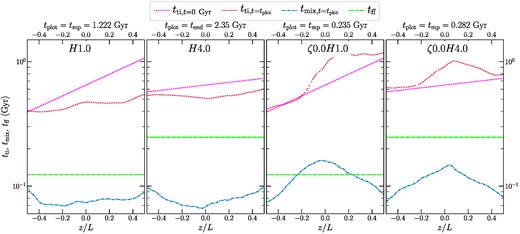
The variation of important time-scales for the hot-phase gas (T ≳ 106 K)–tti, tff and tmix averaged in shells parallel to the z-axis for our fiducial and compressive driving sets of runs at t = 0. For runs in which multiphase gas forms through thermal instability, we also show tti and tmix at the onset of multiphase condensation (at tplot = tmp, denoted in the column titles). For the single phase runs, we show these time-scale profiles at tplot = tend.
We start with an isothermal profile, so at t = 0, tti ∝ ρ−1 (see equation 3a). It varies exponentially with z, with a scale height H. The free-fall time tff is a constant throughout space and time, since we fix |$\boldsymbol {g}$| to a constant value.
For the H1.0 run, the z-gradient of tti flattens and its value decreases slightly, following the same trend as the evolution of the entropy profile shown in Fig. 5. Around the time when cold gas starts condensing out of the medium (t = tmp), tti/tff = 3.87 ± 0.05 and tti/tmix = 5.92 ± 0.08. This medium satisfies the instability criterion (tti/tff ≲ 10) proposed by Sharma et al. (2012) and produces multiphase gas. However, Gaspari et al. (2018) argue that when tti/tmix > 1, turbulent mixing should be able to stop multiphase gas from developing. However, this criterion does not correctly predict the outcome of the H1.0 simulation. By t = tend, cold gas condenses out and falls through the bottom z-boundary. In the new steady state, the hotter and rarer atmosphere has tti ∼ 10 Gyr, tti/tff ≈ 80 (see movie of time-scale profiles evolution in supplementary material or at this link) and is stable against undergoing further thermal condensation.
For the single-phase H4.0 run, the evolution of tti is similar to that of the H1.0 run, but its average value is slightly larger. The ratio tti/tff = 2.19 ± 0.02 and tti/tmix = 6.92 ± 0.04. For this run, the criterion by Gaspari et al. (2018) correctly predicts that multiphase condensation does not occur in this system, while the Sharma et al. (2012) prediction does not hold true.
The amplitude of seed density fluctuations plays a key role in determining whether the systems undergo condensation. The H4.0 run has weaker seed density perturbations compared to the H1.0 run (see row 4 in Fig. 2) and a slightly larger tti/tmix. The relatively faster mixing of the weaker seeds successfully prevents cold gas from condensing out. The two compressive forcing runs have much larger seed density perturbations. Despite having tti/tmix = 6.2 ± 0.5 and 5.4 ± 0.4 at t = tmp for the ζ0.0H1.0 and ζ0.0H4.0 runs, respectively, they both form multiphase gas. At t = tend, the ζ0.0H1.0 run has a similar value of tti as the H1.0 run, albeit with larger variations due to the compressive forcing. In comparison, the ζ0.0H4.0 run reaches a larger tti in steady state, but a similar tti/tff ≈ 100.
3.2 Effect of weaker/stronger forcing
Considering the importance of the turbulence driving for the formation of multiphase gas seen in the previous subsections, here we analyse four more runs, where we vary the strength of the turbulence forcing. In steady state, v ∼ 20–|$40~\mathrm{km\, s^{-1}}$| for the two ‘wdriv’ runs and |$\sim 400~\mathrm{km\, s^{-1}}$| for the two ‘sdriv’ runs. Similar to Fig. 2, in Fig. 7, we show the time evolution of the mcold/mtot, |$\mathcal {M}$|, fturb and σs,hot. We present the z shell-averaged profiles of important time-scales (for the hot phase) in Fig. 8.
Similar to Fig. 2, but for our weak- and strong-driving set of runs. We observe contrasting trends in the development of multiphase condensation with increasing stratification for the weak and strong driving sets of runs.
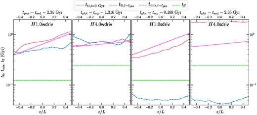
Similar to Fig. 6, but for our for our weak (wdriv) and strong (sdriv) driving sets of runs. For weak driving, the weaker stratification run forms multiphase gas, while for strong driving, the stronger stratification run shows multiphase gas.
Out of the four runs, H4.0wdriv and H1.0sdriv form multiphase gas, whereas H1.0wdriv and H4.0sdriv do not. First, we focus our discussion here on the ‘wdriv’ set of runs. Due to the weak forcing, these two runs are the most comparable to thermal instability studies that do not explicitly drive turbulence (such as Sharma et al. 2012; Choudhury et al. 2019).3
The turbulent eddy turnover time for these two runs is around 0.5–0.7 Gyr. Due to the weaker forcing, turbulence is strongly stratified, with Fr ≪ 1. In this regime, Mohapatra, Federrath & Sharma (2021, fig. 5) showed that density fluctuations decrease with increasing stratification, due to strong buoyancy forces limiting motions in the z-direction.
This is clearly observed in our simulations (fourth row of Fig. 7) as the density fluctuations are smaller for the H1.0wdriv run compared to those for the H4.0wdriv run (for t ≳ 0.8 Gyr). The weaker seed fluctuations are thus unable to induce multiphase condensation in the H1.0wdriv run, even though tti/tff = 6.2 ± 0.1. In Fig. 8, we find that the weak forcing is unable to significantly modify the initial profile of tti by t = tend, unlike the fiducial set, which flattened the z-profiles of tti (and entropy).
For the H4.0wdriv run, tmix ∼ tti around 1.316 Gyr, when the driven turbulence is expected to reach a steady state. Due to the weak turbulent mixing between the z-shells, most of the cold gas condensation occurs from the lower half of the box, which has a smaller initial tti (see movies of simulation in supplementary material or at this playlist link). Compared to the ζ0.0H4.0 run, tti ∼ 2–5 Gyr at t = tend, which is an order of magnitude smaller. Thus, for weaker driving, the system does not lose as much mass to condensation during the simulation period of 2.344 Gyr.
The trend in the two ‘sdriv’ runs are similar to what we observe for the fiducial set – out of the two, the more strongly stratified H1.0sdriv run forms multiphase gas, while the weakly stratified H4.0sdriv run does not. There are a few differences – the initial density fluctuations are larger for the H1.0sdriv run, so the multiphase gas forms much earlier compared to the H1.0 run from the fiducial set even before the z-profile of tti is flattened by turbulent mixing.
Before the onset of multiphase condensation, the amplitude of fluctuations in the H1.0sdriv and H4.0sdriv runs around t = 0.2 Gyr are similar (in agreement with expectations from Mohapatra et al. 2021, for |$\mathcal {M}\sim 1$|). The key difference between the two is the shorter average tti in H1.0sdriv. Although tti/tmix = 9.3 ± 0.2, it is still unable to stop multiphase gas from developing. In the H4.0sdriv run, the turbulent heating due to the strong driving (|$v=410\pm 20~\mathrm{km\, s^{-1}}$|) is more than sufficient to offset the cooling (fturb ≳ 1). The gas heats up with time, showing a gradual decrease in |$\mathcal {M}$| and a larger value of tti at t = tend.
3.3 Effect of weaker cooling
For the runs described in this subsection, we lower ρ0 and P0 by half compared to the fiducial set (so initial T is fixed). This doubles tti, while tff and tmix are unaffected. We show the time evolution of relevant quantities in Fig. 9 and the z shell-averaged time-scale profiles in Fig. 10. These are low-density (or longer tti) counterparts to Figs 2 and 6 for the fiducial set.
Similar to Fig. 2, but for our lower initial density (weaker cooling) set of runs. Only the compressive forcing runs form multiphase gas, albeit at a much later time compared to their fiducial set counterparts.
Similar to Fig. 6, but for our ‘lowdens’ set of runs. The initial density is half compared to the fiducial set, which doubles tti. Only the compressive forcing runs form multiphase gas.
We find that only the two compressive forcing runs form multiphase gas, while the natural forcing runs do not. Since tcool and tti are doubled, tmp ∼ 500 Myr is also doubled for these runs compared to ∼250–300 Myr for the fiducial compressive set with the same parameters. These two runs show a clear decrease in |$\mathcal {M}$| around tmp associated with the hot phase becoming hotter. Since the cooling is weaker, fturb is larger, roughly by a factor of 2 for all the low-density runs compared to their fiducial counterparts. The fraction |$f_\mathrm{turb}\approx 30~{{\ \rm per\ cent}}$| for the natural forcing runs and 50–100 per cent for the compressive forcing runs for t < tmp. For t > tmp, fturb decreases, similar to what we observe for the fiducial set.
In Fig. 10, we find that turbulent mixing flattens the z profiles of tti for both the natural driving runs. The average tti/tff = 6.6 ± 0.2, tti/tmix = 10.4 ± 0.1 for H1.0ldens and tti/tff = 4.52 ± 0.06, tti/tmix = 14.6 ± 0.2 for H4.0ldens run. The larger value of these ratios compared to the fiducial set, ensures that multiphase condensation does not occur in either of these runs.
For the compressive forcing runs, the average values of tti/tff = 13.5 ± 0.6, tti/tmix = 16 ± 3 for ζ0.0H1.0ldens and tti/tff = 6.4 ± 0.3, tti/tmix = 16 ± 2 for ζ0.0H4.0ldens. Both of these ratios are much larger than 1. Both Sharma et al. (2012) and Gaspari et al. (2018) models would predict the ζ0.0H1.0ldens run to not produce multiphase gas, contrary to what we find.4 However, the large density fluctuations due to the compressive forcing grow before either mixing or buoyancy can prevent them from becoming multiphase. By t = tend, tti ∼ 10–30 Gyr similar to that of their fiducial counterparts, despite their longer initial tti. Thus, σs, tti/tff and tti/tmix determine the final value of tti rather than the initial value of tti.
4 SUMMARY OF THE TIME-SCALE RATIOS AND THEIR IMPLICATIONS
Here, we summarize our results from all our simulations and discuss them in the broader context of the conditions that lead to multiphase condensation in the halo gas. In Fig. 11, we show the time taken to form multiphase gas normalized by the thermal instability time-scale (tmp/tti) (first row), minimum values of the ratios tti/tff (second row), tti/tmix (third row), and tti/min (tff, tmix) (fourth row)5 as a function of the standard deviation of logarithmic density (normalized) for all of our 16 simulations. For runs that form multiphase gas, we show these values just before tmp and plot them as filled data points. For the runs that do not form multiphase gas, we plot the ratios at t = tend using unfilled data points. The coloured dashed lines show the time evolution of these quantities as a function of σs prior to multiphase condensation (or the end of the simulation).

First row: Scatter plot of the time taken to form multiphase gas normalized by the z shell-averaged thermal instability time-scale (tmp/tti) versus the standard deviation in the logarithm of gas density (σs) for all our runs. The filled points show runs that form multiphase gas, while the unfilled points show runs that remain single phase till t = tend. For the latter set of runs, we show the lower limits to the ratio, denoted by the upward facing arrows in the symbols. Second row: The minimum value of the ratio of tti to the z shell-averaged free-fall time-scale (tff) tti/tff with the same x-axis. Third row: Similar to the upper panel, but we show min (tti/tmix), the minimum value of the ratio between the z shell-averaged tti and the turbulent mixing time-scale (tmix) instead along the y-axis. Fourth row: Here, we show min (tti/min (tmix, tff)), using the minimum of tff and tmix in the denominator instead. The black line corresponds to the condensation curve described in equation (7a). For the third and fourth rows, the black dashed line is given by equation (7b). It clearly separates between the single phase and multiphase runs in the fourth row. The coloured dashed lines show the time evolution of these ratios as a function of σs till t = min (tmp, tend).
4.1 Time taken to form multiphase gas
Out of our 16 simulations, 9 form multiphase gas. For the seven simulations that remain single phase till t = tend, we plot tend/avg(tti) as a lower limit to tmp/avg(tti), in the first row of Fig. 11. The single-phase simulations are generally concentrated to the upper left part of the figure, whereas the multiphase simulations are to the bottom right. This denotes that larger density fluctuations aid the formation of multiphase gas. Among the runs that form multiphase gas, we find that we can further divide them into three subgroups. The forcing in the four compressive driving runs and the strong driving H1.0sdriv generates large density fluctuations (σs ≳ 0.3) and the gas forms localised high-density pockets with a short cooling time. The multiphase gas forms in tmp ≲ 0.5tti for these simulations. The remaining four multiphase runs form cold gas at tmp ≃ tti. We note that the runs with stronger turbulence (H1.0 and H1.0HR) have stronger density fluctuations but form multiphase gas later compared to the runs with weak or no turbulent forcing (H4.0wdriv and H4.0NoTurb). This highlights that turbulence driving generates stronger density fluctuations but turbulence mixing slows the onset of multiphase condensation. On the other hand, in the absence of mixing the amplitude of density fluctuations keeps growing with time for the H4.0wdriv and H4.0NoTurb runs till t = tmp (see the fourth panel of fig. 7).
4.2 A condensation curve for the formation of multiphase gas
In this subsection, we first discuss how the predictions of thermal instability criteria proposed by Sharma et al. (2012) and Gaspari et al. (2018) hold for our set of simulations. We also attempt to construct a modified condensation curve based on these two criteria for our simulations, taking into account the local variation in tti due to density fluctuations, as well as the lognormal shape of the density distribution (and consequently tcool, since tcool ∝ ρ−1) before multiphase condensation occurs (e.g. see the density PDF for the H4.0 run in fig. 3). Since condensation is a local phenomenon, i.e. dense pockets of gas with a short ratio of the time-scales can condense out even when the atmosphere is globally stable (also seen in Choudhury et al. 2019), we consider the minimum value of these time-scales in our criterion. The densest regions would have gas density ρmax ∼ 〈ρ〉exp (c1σs), where c1 is a positive constant. As tcool ∝ ρ−1, min (tcool) ∼ 〈tcool〉 × exp (− c1σs). Similar to Voit (2021), we use an exponential condensation curve that depends on σs, and which takes into account these local variations in tti (or tcool) due to density fluctuations.
4.2.1 The importance of tti/tff
Sharma et al. (2012) propose the criterion tti/tff ≲ 10 for the onset of multiphase condensation. This is satisfied in all our simulations, barring the ζ0.0H1.0ldens run. Yet 8 out of the 15 simulations do not form multiphase gas, indicating that turbulent mixing has a significant effect on the conditions required for multiphase condensation (also discussed in Banerjee & Sharma 2014; Voit 2018). We find that the simulations that form multiphase gas are concentrated to the bottom right part of the figure, where either σs is large or tti/tff is short. This is in agreement with the findings of Choudhury et al. (2019), who showed that the min (tti/tff) required for cold gas to condense out depends on the amplitude of density fluctuations. They also showed that the min (tti/tff) for which the gas becomes multiphase for a given σs (or amplitude of density fluctuations) rises steeply once σs ≳ 0.5. This effect is seen for our compressive driving run ζ0.0H1.0ldens which has tti/tff > 10 but still undergoes multiphase condensation.
We attempt to construct a condensation curve like in Voit (2021, see their section 4) with the functional form
to separate between the single phase and multiphase runs. We choose c1 = 6 from an empirical fit to our data. However, we have two outlier runs, H1.0 and its high-resolution counterpart H1.0HR that have tti/tff ∼ 2 but still do not form multiphase gas. Since this curve ignores the importance of turbulent mixing of fluctuations, it is unable to predict the occurrence of multiphase condensation correctly for runs with strong turbulent mixing.
4.2.2 The importance of tti/tmix
Now, we discuss the effects of the ratio tti/tmix on the multiphase condensation. As discussed earlier, Gaspari et al. (2018) propose that gaseous haloes become multiphase if tti/tmix ≲ 1 and remain stable otherwise. This criterion does not correctly predict the outcomes of our simulations, since 7 out of the 15 haloes with tti/tmix > 1 form multiphase gas. We think this discrepancy may partly arise because Gaspari et al. (2018) use |$\delta \rho /\rho \propto \mathcal {M}$| (or |$\sigma _s\propto \mathcal {M}$|) to derive the amplitude of density fluctuations in their study (based on the results from cluster-scale simulations in Gaspari & Churazov 2013), which would make the density fluctuations directly related to tmix. This is not in agreement with our results. Recent studies have shown that σs depends on |$\mathcal {M}$|, the degree of stratification (denoted by Fr or HS) (Mohapatra et al. 2020, 2021) and the Mach number of the compressive component of the velocities (Konstandin et al. 2012; Mohapatra et al. 2022b), which correctly predict the amplitude of σs in our simulations. Thus, understanding density fluctuations in cluster environments is key to predicting the thermal stability of the halo gas.
Similar to Section 4.2.1, we attempt to construct a condensation curve of the form min (tti/tmix) = c2exp (c1σs). We set c1 = 6 and c2 = 1.8 empirically. This curve correctly predicts the outcome of simulations with σs ≳ 0.1. However, this criterion ignores the importance of tff. Thus, it fails to predict the outcome of the two runs with weak/no driving and strong gravity (H1.0wdriv and H1.0NoTurb), where min (tti/tmix) ≃ 1 but min (tti/tff) is much larger.
4.2.3 A new condensation curve
Instead of using the two ratios tti/tff and tti/tmix separately, we construct a new ratio tti/min (tmix, tff) by taking the minimum of the two time-scales in the denominator. Our new condensation curve is given by
where c1 = 6 and c2 = 1.8 are empirically determined from fitting our data. As discussed in earlier works and in previous sections of this study, multiphase condensation is inhibited when either of these time-scales are short enough. We plot the minimum value of this new ratio against σs in the third row of Fig. 11. This new condensation curve clearly separates all the simulations into subsets of single phase (unshaded region) and multiphase (grey-shaded region). In the limit of weakly forced turbulence with a long tmix, multiphase condensation is predicted well by the tti/tff ratio. Similarly in the limit of weak stratification, the ratio tti/tmix predicts whether multiphase condensation occurs. Our new combined criterion covers both of these cases.
Although the behaviour of the condensation curve in our study is similar to that of Choudhury et al. (2019) (tmix ≫ tff in their study), we find that our curve flattens to a smaller threshold min (tti/tff) in the limit σs → 0. We think this difference arises because they plot min (tti/tff) and density fluctuations δρ at t = 0 in their condensation curve, whereas we show these values just before multiphase condensation occurs. We expect δρ to grow (for e.g. see H1.0wdriv run in the fourth panel of fig. 7) and min (tti/tff) to decrease by t = tmp, which would make the results consistent with each other.
Predictability of the outcome of a simulation: Here, we discuss whether one can predict the occurrence of multiphase condensation for a given set of simulation parameters – namely Fr, |$\mathcal {M}$|, |$\mathcal {M}_\mathrm{comp}$|, and the ratio of pressure and entropy scale heights RPS. The dashed lines in the second, third, and fourth rows of Fig. 11 show the co-evolution of the corresponding ratios and σs. Except for the H4.0sdriv run, these ratios do not show significant variation with time (after turbulence reaches a roughly steady state). Hence, if one can determine the value of σs using the simulation parameters, then one can predict whether multiphase condensation occurs. We find two expressions for |$\sigma _s^2$| in the literature relevant to the turbulence parameters in our simulations:
from Mohapatra et al. (2021) for subsonic stratified turbulence (where RPS = HP/HS = 0.67 for our simulations) and
from Konstandin et al. (2012) for compressively forced subsonic turbulence. As we show in Fig. 12, equation (7c) agrees well with the the measured value of σs in our natural driving simulations (left column), except the ‘wdriv’ runs. Similarly, equation (7d) accurately predicts the scaling with |$\mathcal {M}_\mathrm{comp}$| for our compressively driven turbulence simulations. The ‘wdriv’ (where turbulence may not have saturated yet) and ‘NoTurb’ runs (where we seed initial density fluctuations by hand) do not show good agreement with either scaling relation.
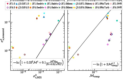
Left column: Scatter plot of the measured logarithmic density fluctuations squared |$\sigma _{s,\mathrm{measured}}^2$| in our simulations versus their predicted value based on the scaling relation in equation (7c). Right column: Scatter plot of |$\sigma _{s,\mathrm{measured}}^2$| vs the compressive component of the rms Mach number |$\mathcal {M}_\mathrm{comp}$|. The dashed line shows the scaling relation in equation (7d). The measured σs shows a remarkable agreement with equation (7c) predicted values for the natural driving runs, except weak turbulent forcing (‘wdriv’ runs, which may not have reached a turbulent steady state yet). On the other hand, the compressive forcing (ζ0.0) runs agree well with the equation (7d). The runs without driven turbulence (‘NoTurb’ runs) do not agree well with either of the scaling relations.
Importance of fturb: Among the simulations that do not form multiphase gas, most reach a steady state where the thermal energy lost due to radiative cooling is replenished by turbulence dissipation and thermal heating. The steady-state value of σs varies only by a few per cent. However, as seen in the third row of Fig. 7, fturb > 1 for the H4.0sdriv run. Thus, the heating rate due to turbulence exceeds the net cooling rate (thermal heating is switched off to prevent further overheating). Initially, the strong turbulence drives large density fluctuations and the pink dashed line initially crosses over to the multiphase side of the condensation curve (in the fourth row of Fig. 11). However, within a few tmix, the gas is overheated, which increases the temperature, decreases |$\mathcal {M}$| and σs, and raises the value of min tti. When fturb > 1, even when the gas properties instantaneously satisfy the condensation criterion, the gas can be heated up on time-scales t < tti, and multiphase condensation is prevented.
5 CAVEATS AND FUTURE WORK
Here, we discuss some of the shortcomings of our study and possible ways to address them. We also outline some future prospects of this work.
5.1 Resolution requirements
In this set of simulations, all our standard set of runs use 5123 × 768 resolution elements to resolve the domain of size 402 × 60 kpc3. So the minimum length that we can resolve is ∼80 pc. In order to capture the turbulent mixing layers between the hot- and cold-phase gas, as well as to reproduce the pressure–temperature phase diagrams, one needs to resolve the cooling length ℓcool, which is orders of magnitude below our resolution limit. In particular, the clear evidence for isochoric cooling in Fig. 4 is an indication that cold gas has collapsed to the grid scale. At that point, the gas cannot be compressed anymore because of insufficient resolution, pressure equilibrium cannot be maintained, and the gas cools isochorically.
Further, the small-scale turbulence is also not well-resolved in this study. Hence, we have not analysed the scale-by-scale kinematics of the hot and cold phases here and leave it to a follow-up study.
We conduct two high-resolution simulations – H1.0HR and H4.0HR with 10242 × 1536 resolution elements. We present these in the Appendix. The results of the higher resolution simulations are similar to those presented in the main text. However, our resolution is still far from what is required to resolve the cooling length ℓcool, so although the convergence in the Appendix is encouraging it is far from a guarantee that the results would be the same if our resolution were sufficient to resolve all the key length scales in the problem.
5.2 Turbulence driving and heating model
Throughout the duration of the simulation, we constantly force turbulence on large scales. Further, to prevent the model from undergoing a global runaway cooling flow, we have applied a shell-by-shell energy balance at all times. Instead of such a fine-tuned balance at all times, clusters are rather expected to undergo cycles of heating and cooling, where a cooling episode triggers strong feedback, heats the gas, and prevents it from further cooling (as seen in simulations, such as Prasad et al. 2015; Beckmann et al. 2019). In a future study, we plan to explore the effect of episodic turbulence driving and decay, to mimic AGN on-off scenarios.
5.3 Missing physics
The density-dependent heating model that we use in our simulations (defined in Section 2.4.4) is quite idealized. We have ignored other possible heating sources such as cosmic rays (Butsky et al. 2020; Kempski & Quataert 2020; Su et al. 2020), thermal conduction (Brüggen & Scannapieco 2016; Jennings et al. 2023), mixing of hot bubbles with the surrounding ICM (Banerjee & Sharma 2014; Hillel & Soker 2017), etc. We have also ignored the effect of magnetic fields in this study. Ji, Oh & McCourt (2018) have shown that magnetic fields, independent of orientation can destabilize buoyant oscillations and modify both the amplitude and morphology of density fluctuations, which are critical to understanding the onset of multiphase condensation. Wang et al. (2021) and Mohapatra et al. (2022a) show that magnetic fields can modify the kinematics of both the hot and cold phases. We plan to conduct follow-up studies exploring the effects of some of these physical elements.
5.4 Geometry
We have modelled the ICM as a plane–parallel atmosphere with constant acceleration due to gravity. However, cluster atmospheres are expected to be spherical/elliptical. Choudhury & Sharma (2016) showed that the amount of cold gas condensing depends on the variation of |$\boldsymbol {g}$| (or tcool/tff) along the radial separation from the cluster centre. The energy and mass budgets are also expected to be different in a spherical atmosphere, since the denser central gas has a smaller mass fraction. The hot gas would be able to expand and cool more easily compared to the plane–parallel atmosphere. We plan to look into the effects of the cluster geometry in a future study.
6 CONCLUDING REMARKS
In this work, we have explored the conditions that lead to cold gas condensation from the thermally unstable hot phase in the intracluster medium. We have conducted 16 idealized simulations of a local box of size (402 × 60) kpc3 including radiative cooling, density-dependent thermal heating and turbulent driving (in 14 out of 16 simulations). The important time-scales that govern multiphase condensation in such a system are (1) thermal instability time tti(∝ tcool, the cooling time); (2) gravitational free-fall time (tff); and (3) turbulent mixing time (tmix). A short tti makes condensation more likely, whereas shorter tff and tmix are expected to prevent condensation. Since tcool ∝ ρ−1 (gas density), the amplitude of logarithmic density fluctuations σs is also an important parameter to determine local variations in tti. The ratios between the aforementioned time-scales of the system – tti/tff and tti/tmix are important to predict the occurrence of multi-phase condensation. Here, we summarize the main takeaway points of this work, focusing on the importance of these ratios:
In the limit of weak stratification, the ratio tti/tmix predicts the occurrence of multiphase condensation. We find that turbulent mixing suppresses multiphase gas condensation even for runs with min (tti/tff) ≃ 2 (see H4.0 run in Figs 2 and 6). This result is further corroborated by our findings in our strong turbulent driving set of runs (labelled ‘sdriv’, see Figs 7 and 8).
In our weak turbulence driving simulations (labelled ‘wdriv’) and simulations without constantly driven turbulence (labelled ‘NoTurb’), we find the occurrence of multiphase condensation is predicted well by the tti/tff ratio (see Figs 7 and 8). Strong stratification suppresses multiphase condensation even when min (tti/tmix) ≃ 1 in our H1.0wdriv and H1.0NoTurb runs.
Large density fluctuations always increase the likelihood of multiphase condensation. Cold gas forms in our simulations with min (tti/tmix) ≳ 1 and min (tti/tff) ≳ 10, if the turbulence driving promotes strong density fluctuations, such as for compressive driving (see ζ0.0 runs in Figs 2, 6, 9, and 10). This happens due to the formation of dense pockets of cold gas with short tti. The dependence of multiphase condensation on σs is clearly seen in Fig. 11.
Thus the two ratios min (tti/tff) and min (tti/tmix) collectively predict whether multiphase condensation occurs. In the limit that one of these ratios is much larger than the other, the larger of the two determines whether multiphase gas forms. Taking into account our findings above, we propose a new condensation criterion that considers the importance of both tff and tmix as well as the variability in tti due to large density fluctuations, which we parameterize using σs. Our new multiphase condensation criterion is given by min (tti/min (tmix, tff)) = c2 × exp (c1σs) with c1 = 6 and c2 = 1.8, empirically determined and shown in the bottom panel of Fig. 11. When the minimum value of the ratio tti/min (tmix, tff) falls below this threshold, multiphase condensation occurs in our simulations.
Unlike previous studies, we find that the entropy scale height does not always play a significant role in determining whether or not a system forms multiphase gas. Turbulent mixing flattens the entropy gradient on scales smaller than the driving scale in a few mixing time-scales. However, in the limit of weak or no turbulence, simulations with a steeper entropy gradient are more stable against thermal condensation.
Our simulations that form multiphase gas reach a second steady state after most of the condensed cold gas rains down through the bottom z-boundary. In this state, we find the value of min (tti/min (tmix, tff)) to be independent of the initial value of min (tti/(tmix, tff)) (before the condensation begins). Instead, its steady-state value increases with the amplitude of turbulent density fluctuations.
ADDITIONAL LINKS
Movies of projected density and temperature as well as time-evolution of z-averaged time-scale profiles of different simulations are available as online supplementary material, as well as at the following links:
Playlist of fiducial runs and compressive driving (ζ0.0) sets of runs;
Playlist of weak (‘wdriv’) and strong (‘sdriv’) driving sets of runs;
Playlist of low-density (‘ldens’) sets of runs;
Playlist of high-resolution (‘HR’) runs.
Playlist of runs without external driving ‘NoTurb’.
ACKNOWLEDGEMENTS
PS acknowledges a Swarnajayanti Fellowship (DST/SJF/PSA-03/2016-17) and a National Supercomputing Mission (NSM) grant from the Department of Science and Technology, India. CF acknowledges funding provided by the Australian Research Council (Future Fellowship FT180100495 and Discovery Projects DP230102280), and the Australia-Germany Joint Research Cooperation Scheme (UA-DAAD). This work was supported in part by a Simons Investigator award from the Simons Foundation (EQ) and by NSF grant AST-2107872. We further acknowledge high-performance computing resources provided by the Leibniz Rechenzentrum and the Gauss Centre for Supercomputing (grants pr32lo, pr48pi, and GCS Large-scale project 10391), the Australian National Computational Infrastructure (grant ek9), and the Pawsey Supercomputing Centre (project pawsey0810) in the framework of the National Computational Merit Allocation Scheme and the ANU Merit Allocation Scheme. The analysis presented in this article was performed in part on computational resources managed and supported by Princeton Research Computing, a consortium of groups including the Princeton Institute for Computational Science and Engineering (PICSciE) and the Office of Information Technology’s High Performance Computing Center and Visualization Laboratory at Princeton University. The simulation software, flash, was in part developed by the Flash Centre for Computational Science at the Department of Physics and Astronomy of the University of Rochester.
This work used the following software/packages: flash (Fryxell et al. 2000; Dubey et al. 2008), matplotlib (Hunter 2007), cmasher (van der Velden 2020), scipy (Virtanen et al. 2020), numpy (Harris et al. 2020), h5py (Collette 2013), and astropy (Astropy Collaboration 2018).
DATA AVAILABILITY
All relevant data associated with this article is available upon reasonable request to the corresponding author.
Footnotes
The turbulence driving module is publicly available on GitHub (Federrath et al. 2022).
Note that we expect turbulence to grow and reach a steady state in roughly 2–3 eddy turnover time-scales (Federrath et al. 2010), which corresponds to 150–250 Myr for our fiducial set of runs. For some of our runs, this time-scale is longer than tmp. For such runs, we calculate the time and volume-averaged quantities in the last 25 Myr just before tmp, to reduce the effect of unsaturated turbulence-evolution on the time-averaging.
For a direct comparison with Sharma et al. (2012) and Choudhury et al. (2019), we have also conducted two simulations ‘H1.0NoTurb’ and ‘H4.0NoTurb’ where we only introduce seed density fluctuations and do not drive turbulence explicitly. The results from these simulations are consistent with the corresponding ‘wdriv’ set of runs and are also in agreement with the aforementioned studies of thermal instability.
Although the z shell-averaged values of tti/tff and tti/tmix are large, these ratios can become much smaller in dense, locally compressed regions produced by the compressive forcing.
Note that we calculate the minimum value of these ratios using the z-shell averaged values of tti and tmix instead of calculating their minimum values over the entire domain. This makes our results directly comparable to the radial profiles of the time-scales obtained from observations. The local variations in tti are mostly due to density fluctuations, which are captured well by σs.
References
APPENDIX A: CONVERGENCE TEST WITH RESOLUTION
Here, we check the convergence of the results of our fiducial set of runs by doubling the resolution of our simulations. Similar to our fiducial set, the H1.0HR run becomes multiphase whereas the H4.0HR run remains single phase till t = tend.
We show the time-evolution of the different volume averaged quantities in Fig. A1. For the single phase H4.0 and H4.0HR runs, the evolution of these quantities are quite similar and almost overlapping throughout the duration of the simulation. The H1.0HR run forms cold gas slightly later compared to the H1.0 run. However, the steady state values of all quantities before and after the formation of cold-phase gas are similar, so the results are largely in agreement.
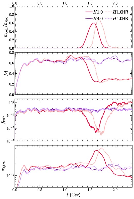
Similar to Fig. 2, but for our fiducial set and a higher resolution (HR) set of runs. These volume-averaged quantities are largely convergent with resolution.
In Fig. A2, we show the high-resolution counterpart of Fig. 1. Clearly, the cold gas collapses to smaller scales upon increasing resolution. We have already discussed regarding this effect in Sections 3.1.4 and 5. When the cooling length of the gas is not resolved, it collapses to the grid scale and cannot be compressed anymore.
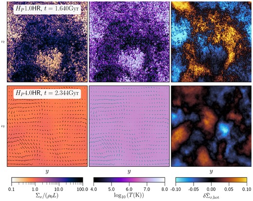
Similar to Fig. 1, but for our high-resolution set of runs. For the multiphase H1.0HR run, the cold gas collapses to smaller scales compared to its fiducial counterpart H1.0.
