


ABSTRACT
The solar inner corona is a region that plays a critical role in energizing the solar wind and propelling it to supersonic and supra-Alfvénic velocities. Despite its importance, this region remains poorly understood because of being least explored due to observational limitations. The coronal radio-sounding technique in this context becomes useful as it helps in providing information in parts of this least explored region. To shed light on the dynamics of the solar wind in the inner corona, we conducted a study using data obtained from coronal radio-sounding experiments carried out by the Akatsuki spacecraft during the 2021 Venus-solar conjunction event. By analysing X-band radio signals recorded at two ground stations (Indian Deep Space Network in Bangalore and Usuda Deep Space Center in Japan), we investigated plasma turbulence characteristics and estimated flow speed measurements based on isotropic quasi-static turbulence models. Our analysis revealed that the speed of the solar wind in the inner corona (at heliocentric distances from 5 to 13 solar radii), ranging from 220 to 550 km s−1, was higher than the expected average flow speeds in this region. By integrating our radio-sounding results with extreme ultraviolet (EUV) images of the solar disc, we gained a unique perspective on the properties and energization of high-velocity plasma streams originating from coronal holes. We tracked the evolution of fast solar wind streams emanating from an extended coronal hole as they propagated to increasing heliocentric distances. Our study provides unique insights into the least-explored inner coronal region by corroborating radio-sounding results with EUV observations of the corona.
1 INTRODUCTION
The unusually high temperature of the solar corona does not let it end at a sharp boundary; instead, it continues outward to the interplanetary medium. This thermally driven flow of ionized particles is termed the solar wind (Parker 1958). Observations made from space confirmed that this ubiquitous flow of charged particles in the form of solar wind pervades the entire interplanetary medium at all the helio-latitudes and helio-longitudes (McComas et al. 2000). These observations also revealed the fact that the specific regions in corona give rise to various kinds of solar wind streams. Solar wind observations near 1 au have identified three main types of solar wind based on differences in their speeds and densities: the fast solar wind, with speeds > 400–700 km s−1, the slow solar wind, with speeds around 400 km s−1, and transient wind that occurs during coronal mass ejections (Marsch 1999). These different types of wind are thought to originate from different regions of the corona. For example, fast solar wind typically originates in coronal holes, which are darker regions [as viewed in the extreme ultraviolet (EUV) and soft X-ray coronal images] of the Sun at higher helio-latitudes with open magnetic field lines (Zirker 1977). Slow solar wind, on the other hand, originates above the active regions in the streamer belts, which are mostly found near the low-equatorial helio-latitudes (Geiss, Gloeckler & von Steiger 1995). The characteristics and extent of these coronal features are determined by the convective activity of magnetized plasma that surfaces from the photosphere beneath the corona. The relative motion and abundance of these features depend on various factors, including the phase of the solar activity cycle, the number of sunspots, and the frequency of magnetic reconnection processes occurring on the solar surface (McComas et al. 2003; Antiochos et al. 2011).
It is also observed that solar wind plasma velocities beyond 20–30 R⊙ (1 R⊙ = 1 solar radii = 696 700 km) and near-Earth regions are mostly supersonic and super-Alfvénic, with average magnitudes of between 400 and 700 km s−1, corresponding to slow and fast wind, respectively. The solar wind in the inner corona, on the other hand, is subsonic (Woo 1995; Sheeley et al. 1997). The acceleration of solar wind particles from subsonic to supersonic and super-Alfvén velocities occur in the transition region (McIntosh et al. 2011; Kasper et al. 2021). Thus, mapping solar wind speeds near the Sun becomes crucial to understanding its origin and expansion.
According to Parker’s hydrodynamic corona theory, the high temperature of the corona is the main factor responsible for accelerating the solar wind by creating a pressure gradient that propels ionized charged particles outward from the corona and toward the interplanetary medium (Parker 1958). However, the physics behind coronal heating mechanisms, solar wind acceleration processes, and phenomena occurring at the transition of the solar wind at the critical Alfvénic surface (Adhikari, Zank & Zhao 2019) still require deeper understanding. Various mechanisms have been proposed, with the most prominent attributing coronal heating to turbulence and the dissipation of energy contained in magnetohydrodynamic (MHD) waves that traverse the low-beta plasma region (Cranmer et al. 2015). Some models also consider small-scale impulsive energy releases by magnetic reconnection during nanoflare events (Sakurai 2017). Recently, the XSM instrument onboard Chandrayaan-2 has detected a large number of microflares (sub-A class flares) during the deepest minima of the last century (Vadawale et al. 2021). Estimates on nanoflare heating of the corona (Upendran et al. 2022) have also been made, providing further evidence for the nanoflare mechanism.
There are several ways in which MHD waves mediate turbulence, such as interaction of forward propagating Alfvénic waves with counter-propagating waves, partial reflection due to coronal inhomogeneity, mode coupling/phase mixing in regions of strong gradients of density and magnetic field, and especially for low beta plasmas parametric decay instability (PDI) mechanism, leading to the to the energization of the solar wind in the solar corona. These mechanisms have a rich scientific basis and many detailed studies are available (Hollweg 1986; Matthaeus et al. 1999; Cranmer et al. 2015; Shoda et al. 2019). Among them the conversion of Alfvén waves into compressed ion acoustic waves and their dissipation of shock waves emerges as significant one. The Alfvén waves, which are transverse waves, carry photospheric magnetic field into the base of the corona and the transition region. The energy fluxes transported by the Alfvén waves are sufficient to energize the quiet corona and power the fast solar wind (McIntosh et al. 2011). Non-linear processes in the turbulent plasma cause Aflvénic waves to decompose into forward propagating compressive magnetosonic waves and backward propagating Alfvénic waves (Shoda et al. 2019). The interactions between the outgoing and incoming wave-packets sets up the turbulence in the medium. Turbulence, in turn, assists in the energy cascading process and magnetosonic waves dampen and dissipate energy leading to high temperatures in corona (Coleman 1968; Cranmer, van Ballegooijen & Edgar 2007), and also causes a wave pressure gradient that accelerates the wind (Alazraki & Couturier 1971; Belcher 1971). Several models based on simulation of MHD waves turbulence and dissipation (Roberts et al. 1992; Cranmer et al. 2007; Verdini & Velli 2007; Chandran & Perez 2019; Shoda et al. 2019) have been proposed to explain this phenomenon of plasma turbulence, energy dissipation, and acceleration of solar wind.
The harsh conditions in the solar corona, including high temperatures and a complex magnetic field, have made in situ measurements challenging. In this context, coronal radio-sounding techniques have proven invaluable for obtaining information about the near Sun coronal medium, where direct plasma measurements are difficult. Early studies used radio emissions from natural sources like the Crab Nebula and quasars to investigate interplanetary scintillations (IPS) at different distances from the Sun (Hewish, Scott & Wills 1964). Subsequently, it was realized that higher frequency and more stable radio beacons, such as spacecraft signals during radio occultation in the S, X, and Ka bands, can be utilized to probe regions of the inner corona with higher electron densities (Bird et al. 1992). Previous missions have utilized downlink radio signals from spacecraft during solar conjunction periods to conduct studies on the solar corona (Pätzold, Tsurutani & Bird 1997; Chashei I.V, Plettemeier & Bird 2005; Imamura et al. 2005; Efimov et al. 2005b, 2008; Pätzold et al. 2012; Wexler et al. 2019b). Solar conjunction refers to the period when a planet (and hence the spacecraft orbiting that planet), the Sun, and the Earth align in a straight line, with the Sun at the centre. Radio signals transmitted from the spacecraft pass through the solar corona during this period (Fig. 1). As the corona is an ionized medium with fluctuating electron density, it induces dispersive signatures in the radio signals. These signatures can be analysed to study various coronal properties, including plasma turbulence regimes, velocity, density, magnetic field fluctuations, and solar wind acceleration (Woo & Armstrong 1979; Bird 1982; Bird & Edenhofer 1990; Wohlmuth et al. 2001; Efimov et al. 2005a).
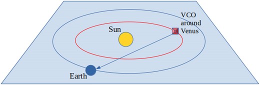
Schematic of Venus–Sun–Earth during 2021 Venus–solar conjunction in the ecliptic plane. VCO (Akatsuki) spacecraft is orbiting around Venus.
In this study, we used the single downlink X-band radio signals transmitted by the Akatsuki spacecraft [also known as Venus Climate Orbiter (VCO)] to study coronal properties during Venus–solar conjunction that occurred in 2021 March–April. This is the period that corresponds to the ascending phase of solar cycle 25 when the solar activity started increasing after minima of comparatively weaker solar cycle 24. A serendipitous observation has been the fast solar wind during the period of study which gave us an opportunity to track the evolution of the fast solar wind speed from the source to different heliocentric distances to the L1 point in the near-Earth environment as observed during the experiment period. The radio-sounding data were collected simultaneously at two stations – IDSN (Indian Deep Space Network), Bangalore, and at UDSC (Usuda Deep Space Center), Japan. Here, we have studied the plasma turbulence characteristics and estimated the flow speeds at the heliocentric regions as close as 5–13 R⊙ using radio signals received at IDSN Bangalore as discussed in further sections.
2 DATA PROCESSING AND OBSERVATIONS
The experiment was performed using the Akatsuki orbiter which is a Japanese satellite orbiting Venus (Nakamura et al. 2011). During the 2021 Venus–solar conjunction, the solar occultation experiments were performed using the radio science payload onboard Akatsuki (Imamura et al. 2011). It uses an onboard ultra-stable oscillator (USO) to generate radio signals at X-band (8410 MHz) frequencies. Experiments are conducted in one-way downlink mode and signals are recorded at IDSN and UDSC, simultaneously or individually depending upon the satellite’s orbit geometry vis-a-vis station visibility. Further details of the payload, technical specifications, and data analysis methods are given elsewhere (Imamura et al. 2011, 2017; Tripathi, Choudhary & Jayalal 2022). This conjunction geometry is important in two aspects: first, the solar proximate distance, i.e. tangential distance of the closest point of radio ray path from the center of the Sun, is as close as 4–13 R⊙ and crosses the helio-latitudes between 24°–86° S. Such a geometry provided us with a good opportunity to probe the spatial variations in plasma conditions near southern solar hemisphere corona. Fig. 2 depicts the relative position of spacecraft and the Sun as seen from Earth’s sky plane. Second, this experiment was performed during 2021 March, a period that corresponds to the ascending phase of solar cycle 25 (solar cycle 24 minima was in 2019). During our observation period, solar 10.7 cm flux was 76.5 SFU (1 SFU = 10−22 Watts m−2 Hz−1) and the average sunspot number was 17.2 (https://www.swpc.noaa.gov/products/solar-cycle-progression). No strong Coronal Mass Ejections (CME) event was recorded during this period, thus no transient wind existed and this makes it an ideal situation to study the background solar winds in quiet solar conditions.
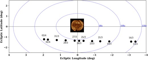
Akatsuki–solar conjunction geometry during 2021 March–April. Circles show apparent position of Akatsuki (in DD–MM format) as seen from plane of sky on Earth with respect to the Sun at 00:00 UTC on experiment days in Solar Ecliptic (ECLIPJ2000) coordinate system. SDO/AIA image of coronal disc on 2021 March 27 is embedded depicting Sun. Concentric circles are constant heliocentric distance contours drawn at every 5 R⊙.
The radio signal data were recorded simultaneously at the IDSN, Bangalore and UDSC, Japan using open-loop receiver systems in the standard CCSDS–RDEF (raw data exchange format) format (https://public.ccsds.org/Pubs/506x1b1.pdf). The data collected at these stations were later used to calculate the experimentally recorded observed Doppler frequency fluctuations imprinted on radio signals passing through the solar corona, by adopting standard processing methods as given in (Pätzold et al. 2004; Choudhary et al. 2016; Tripathi et al. 2022). The observed Doppler was extracted at the sample rate of 1 Hz. For each station, theoretical Doppler (range rate Doppler, or Doppler arising due to relative motion of spacecraft and receiver) was calculated using spice kernels provided by UDSC/IDSN teams (Acton 1996). The difference between observed and theoretical Doppler gives an observable quantity of ‘differential Doppler-frequency residual’ values, that separates the non-dispersive Doppler from the dispersive effects (Tripathi et al. 2022). The appropriate fit was calculated and subtracted from processed Doppler-frequency residual values to compensate standard sources of error for the oscillator drifts, other imperfections in trajectory, and the effects of the terrestrial ionosphere and atmosphere (Tripathi & Choudhary 2022). We obtained fluctuations of these frequency residual values around zero mean termed frequency fluctuations (FFs), a parameter that contains the dispersive effects arising due to the turbulence in the propagating medium. The proximate distance of radio ray path from the solar centre (termed solar offset) in terms of heliocentric distances is calculated using the ephemeris of the Akatsuki spacecraft and planetary ephemeris as offered in NASA spice tool (Acton 1996). The results of the turbulence regimes have been quite successfully used by the radio-science community to understand various phenomena such as electron density fluctuation spectra (Woo & Armstrong 1979), phase scintillation spectra (Pätzold, Karl & Bird 1996), temporal spectra of fluctuations amplitude of radio signals (Yakovlev et al. 1980), and magnetic field power spectra (Chashei et al. 2000; Wexler et al. 2019a) using recorded Faraday rotation in the received signal from solar-conjunction experiments. In this work, we used these FF values to characterize the turbulence spectrum spectra and estimate the plasma flow speeds in the inner coronal region using the methodologies as prescribed in the radio-sounding data analysis (Wexler et al. 2019b).
3 RESULTS
As mentioned, in this study we utilized the observable parameter obtained from our radio occultation experiments, the Doppler FF. Fast Fourier transform was applied to these FFs. The resultant temporal spectrum of Fourier transformed values of FF was approximated as the single power-law spectrum between frequency range [νlow, νup]. The frequency range to apply power-law approximation is defined such that the lower frequency cut-off νlo = 10−3 Hz is the length of the processed interval and upper νup = 5 × 10⁻² Hz is bounded by one-tenth of Nyquist frequency under consideration of the fact that above which system noises will dominate the fluctuation data (Efimov et al. 2008). The linear fit on the log–log plot gives a slope that is an exponential index (αf) of the single power-law spectrum of recorded frequency fluctuations. αf is related to the spectral index of electron density turbulence spectrum p as αf = p − 3 for 3D turbulence (Efimov et al. 2008; Jain et al. 2022).
Table 1 shows the values of the subsequent spectral index for all the experimental days. It can be observed that spectrum has slope values ranging from 0.12–0.30 for the entire duration of conjunction experiment.
Index of temporal spectrum of frequency fluctuations recorded at IDSN station obtained from Akatsuki Solar-Conjunction 2021 experiment. Values of heliocentric distance R⊙ of ray path proximate point and spectral index corresponding to each experiment day are tabulated.
| Date | R(R⊙) | Spectral index (αf) |
|---|---|---|
| 2021 March 14 | 12.82 | 0.24 |
| 2021 March 19 | 8.71 | 0.29 |
| 2021 March 21 | 7.24 | 0.16 |
| 2021 March 23 | 6.09 | 0.12 |
| 2021 March 25 | 5.28 | 0.21 |
| 2021 March 26 | 5.09 | 0.23 |
| 2021 March 27 | 5.08 | 0.20 |
| 2021 March 29 | 5.57 | 0.18 |
| 2021 March 31 | 6.62 | 0.28 |
| 2021 April 02 | 7.98 | 0.13 |
The theory of solar wind acceleration by the MHD waves and turbulence states that the turbulence is caused by the ensemble of Alfvén and magnetosonic waves entrained in the solar wind. The transition from the acceleration region to the steady-flow region is accompanied by the spatial change in turbulence regime (Chashei & Shishov 1983), as reflected by the changes in the slope of the turbulence spectrum. It is known that for the inner coronal regions, the spectral index values are generally lower and appear as flatter slopes in the turbulence spectrum. Lower αf (∼0.2−0.3) values in temporal frequency fluctuation spectra denote the energy source/input regime where turbulence is still underdeveloped (Armand, Efimov & Iakovlev 1987). With the increasing heliocentric distances, the cascading of energy sets up, and thus the slope value starts increasing. The spectral index of a fully developed 3D Kolmogorov electron density turbulence spectrum is p = 11/3 (Woo et al. 1976). This corresponds to the spectral index αf ∼ 0.6−0.7 of frequency fluctuation spectrum which denotes an inertial range of developed turbulence regime and occurs generally around the transition region beyond 10 R⊙ (Efimov et al. 2008). Previous solar occultation studies from spacecraft (Efimov et al. 2005a; Jain et al. 2022) have shown that as we move away from the solar surface, with the increasing heliocentric distances the slope of plasma turbulence spectrum gets steeper and transition to the Kolmogorov values usually occur around 10–15 R⊙ (Imamura et al. 2005).
However, in our case, we found that the turbulence spectrum was flatter for the entire range of 5−13 R⊙ heliocentric distances. Fig. 3 shows the turbulence spectrum for three such experiment days where each day represents the different solar proximate distance. It can be noted that at closer heliocentric distances (first spectrum when R = 5.09 R⊙ the slope is 0.23), the spectrum is flatter. With the increasing heliocentric distances it is expected that slope values increase which should manifest as steeper spectrums. However, for the other two spectra in Fig. 3 (when R = 8.71 R⊙ the slope is 0.29 and when R = 12.80 R⊙ the slope is 0.24) it is observed that with increasing heliocentric distances the turbulence spectrum remains still flatter.
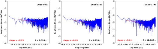
Temporal spectrum of FF on three experiment days corresponding to the increasing heliocentric distance of proximate ray path point, (a) when R = 5.09 R⊙ the index is 0.23, (b) when R = 8.71 R⊙ the index is 0.29, (c) when R = 12.80 R⊙ the index is 0.24. The flatter slope values even with increasing heliocentric spectrum indicates the radio ray path was embedded in the region of fast solar wind.
The intriguing nature of this observation prompted us to investigate the existing coronal dynamics conditions prevailing during the experimental days with respect to helio-latitudes and coronal features of the proximate point of the radio ray path. Previous studies on the turbulence characteristics of inner solar wind plasma, which observed the dependence of spectral index with respect to the helio-latitudes, have reported that at the higher helio-latidues, the spectral index values are generally lower (Pätzold et al. 1996; Efimov et al. 2010). During an ascending phase of the solar cycle, when the solar activity is lower, higher helio-latitudes are dominated by the features known as coronal holes, which are sources of fast solar winds. The fast solar winds emanate from the coronal holes which are regions of open field lines. This leads to the lower values of the sound waves to Aflvénic wave speed ratio and thus turbulence takes a longer time (hence larger heliocentric distances) to achieve a fully developed spectrum. Hence, previous studies (Pätzold et al. 1996; Efimov et al. 2010) have shown that at higher helio-latitudes the turbulence spectrum is expected to still be an underdeveloped regime and is indicated by the flatter slopes. The change in the turbulence regime takes place at farther greater distances from the solar surface for the fast solar wind than for the slow solar wind.
To put the discussions in context, we estimated the solar wind flow speeds from our spectral index calculations. Section 4 discusses the estimation of solar wind flow speeds using a well known formulation, known as the isotropic quasi-static turbulence model, which is based on the propagation of EWs through a turbulent plasma medium and is readily employed in studying the turbulence characteristics of inner solar wind (Chashei & Shishov 1983; Armand et al. 1987). It is worth mentioning here that the solar wind speed can be estimated from the intensity scintillation spectrum as well, as done by Chiba et al. (2022). The results will be reported elsewhere.
4 DISCUSSIONS
Our study shows that the turbulence spectra for the given heliocentric distances of solar offsets are generally flatter. This is interesting because there should have been a gradual increase in the slope values with the increasing heliocentric distances (Jain et al. 2022). As a flatter slope indicates the source region in the turbulence regime, we need to understand why the solar wind remains in the source region of energization and how the solar wind during this period evolves with varying heliocentric distances.
Turbulence is a pervasive characteristic of heliospheric plasma across all heliocentric distances and latitudes (Efimov et al. 2005b), and turbulence models employed in the study of solar wind plasma successfully capture the energy transfer in MHD waves, the heating of the solar corona, and the outward acceleration of the solar wind. At closer heliocentric distances near the active source regions, Aflvén waves emerge from the base of the solar corona carrying large amounts of energy. As they propagate forward, the magnetic field energy decreases, and the non-linear processes such as parametric decay instability activates in the low-beta plasma. Then a forward propagating Alfvén wave is converted into a backward propagating MHD wave and forward propagating ion coustic (magnetosonic both compressive and non-compressive modes) waves. These magnetosonic waves propagate longitudinally to create random density and magnetic fluctuations in plasma, thereby further setting up a turbulence cascade in the medium. The energy contained in magnetosonic waves is then transferred into the lower wavelengths which dissipates and heats up the corona, leading to the acceleration of solar wind particles (Coleman 1968; Derby 1978; Goldstein 1978; Chashei & Shishov 1983; Jain et al. 2022).
4.1 Velocity estimation from two-station cross correlations and its limitations
As mentioned earlier, the signal transmitted from the Akatsuki spacecraft during the coronal-sounding experiment was received simultaneously at two stations – UDSC (Japan) and IDSN (India). This encouraged us to use one subclass of these coronal-sounding experiments, the very long baseline interferometer (VLBI) technique to estimate flow speeds (Spangler et al. 2002). In this technique, the radio signal transmitted by the spacecraft is received simultaneously at two spatially separated ground stations. The radio signals received at two antennas are then correlated to deduce the observable difference in the Doppler phase of two signals received, which can be attributed to the turbulent plasma irregularities that are embedded in the solar wind and advected radially across the line of sight (LOS) of two antennas. The frequency residuals and cross-correlation functions are calculated in overlapping time intervals of the same experiment day for both stations. It is assumed that the density homogeneity of the medium, which causes frequency fluctuation in the received radio signal, is a ‘frozen-in’ solar plasma medium and is convected outwards in a direction perpendicular to the signal ray path with solar wind speed. The coronal separation of ray path proximate points ΔR at the time when signals are received at two stations, combined with a correlation time lag τ, assists in estimating the average outward flow speeds (Vsw = ΔR/τ) of inner solar wind (Janardhan et al. 1999; Efimov et al. 2010; Ma et al. 2021).
We used a similar approach with our Doppler residual data. It was however found that the cross-correlation between the two station data was consistently weak and correlation coefficient values were poor. The weak correlation made the determination of correlation time lag values uncertain and hence we were not able to use this method to calculate the flow speeds conclusively. One of the reasons for this weak cross-correlation in two data sets can be the absence of this density inhomogeneities markers across the radio ray path in the region of the coronal medium which is being probed (Janardhan et al. 1999). To support this observation, we considered the autocorrelation of the single station data and found out that the correlation coherence length, which is indicative of the spatial span and lifetime of the discernible inhomogeneity plasma tracer to travel across separation between two radio ray paths, was actually too narrow to estimate flow speeds. For instance, Fig. 4 represents the autocorrelation of the Doppler frequency fluctuations recorded at the IDSN station on experiment day of 2021 March 19, when the area probed by radio signals is around 8.7 R⊙. During this day the average coronal separation of the two radio paths, one at IDSN and the other at UDSC station, was ΔR = 2636 km. The autocorrelation of frequency residual values at IDSN station yields the coherence length of Δτ < 1 s. If we assume that the average solar wind speed at this coronal region is approximately 200 km s−1 (Sheeley et al. 1997), the spatial tracer span should be approximately 200 km or less, this points that the average spatial span of inhomogeneity tracers is less than the coronal separation. This further indicates the absence of significant turbulent plasma tracers and hence the weak cross-correlation between the two station data. Having said so, we do not imply a complete non-existence of such structures in the solar plasma. There is a possibility that these structures exist but they might decay so rapidly that their signatures are not recorded in the next station. Either way, in this experiment we could not detect any significant autocorrelation, which led to the conclusion that the cross-correlation technique in our present case was not able to yield significant solar wind velocities results, as done in the VLBI technique. It was in fact, noticed during the entire period of our study and made us ponder that the radio-ray path is embedded in the region of solar wind where turbulence is still underdeveloped and in the source regime of turbulence spectrum.

Upper panel: Frequency fluctuation residual values from the radio signal obtained from IDSN station. Lower panel: Autocorrelation of Doppler frequency residuals obtained from radio signal received at IDSN station on 2021 March 19, from the Akatsuki coronal sounding experiment.
Since the methodology based on cross-correlation of two station data posed some limitations in our case to use the VLBI technique for estimating the velocities in the inner corona, we decided to adopt another approach based on the isotropic quasi-static turbulence model which uses single station data to estimate the solar wind velocities.
4.2 Isotropic quasi-static turbulence model
The dispersion relation of any plasma medium is the function of plasma frequency (i.e. the function of plasma densities) and the frequency of the incident electromagnetic wave (EW; Chen 1974). For an EW passing through the coronal medium, as the turbulence is its inherent quantity at all helio-latitudes and heliocentric distances (Coleman 1968; Cranmer et al. 2007; Bruno & Carbone 2013), the turbulent ionized medium induces dispersive effects in the phase and frequency of the traversing wave (Tatarski 1971). The impact of plasma density turbulence thus remains imprinted on the fluctuations in the phase of the emergent EWs (corresponding to the Doppler shift in the frequency domain). These phase fluctuations thus can be analysed to study the turbulence characteristics.
We considered one of the well known models for studying solar wind turbulence – the isotropic 3D quasi-static turbulence model as provided by the (Armand et al. 1987; Chashei, Efimov & Bird 2007; Efimov et al. 2008, 2010). This model assumes a bulk outflow of ‘frozen-in’ turbulence radially away from the coronal surface. It takes into account density inhomogeneities that follow a quasi-static isotropic turbulence pattern. The model was used to study the temporal frequency fluctuation turbulence spectra and extended further to estimate the plasma flow speeds perpendicular to the LOS of the radio ray path using an approach as provided by (Wexler et al. 2019b). Here, it is assumed that the electron density inhomogeneities have 3D turbulence spectra and are advected perpendicularly to the LOS of the radio ray path with the background solar wind flow speeds.
The phase of EWs of original transmitted frequency fo are related to the phase of the received signal frequency fr by the rate of the change of relative spacecraft and receiver velocity Vrel called as range rate Doppler along the LOS and rate of change refractive index, which is related to the electron density of the medium (Chashei et al. 2007; Wexler et al. 2019b). We based our analysis on the FF model of quasi-static isotropic turbulence as given in (Wexler et al. 2019b), accordingly:
Here, λ = c/fo is the transmitted frequency wavelength, c is the speed of light, and ne is the electron number density in the solar corona along the LOS length. Due to inherent turbulence in the medium, the density term ne includes a mean component and a fluctuating component of amplitude δne that contribute to the fluctuating component of FF, and ds is the vertical LOS integration path increment. LLOS is taken to be the magnetically determined correlation length, re is the classical electron radius, re = e2/(4πϵomec2). If we remove the contribution arising due to the range rate Doppler (also mentioned as theoretical/geometrical), the instantaneous change in FF is δf(t) = fobs(t) − fo. Considering the density fluctuation term of the form δne(t) = δneexp−iωt, the time derivative relation of the FF becomes,
To analyse the power spectrum, we proceeded with the Fourier transform of the above equation. The power spectral density for a given data segment of temporal length T is denoted as |$|FF(\omega)|^2 = (1/T) (\mathcal {F}\lbrace \delta f(t)\rbrace) (\mathcal {F}^{*}\lbrace \delta f(t)\rbrace)$|,
where |δne(ω)|2 is the corresponding power spectral density of electron concentration fluctuations.
This is the equation of density fluctuation of a single slab. We denoted FF in terms of oscillation frequency in Hz, ν = ω/2π. These FFs are converted to radio wavelength normalized fluctuation measure FM (by using |$\sigma _{\mathrm{ FM}} = \sqrt{\sigma ^2_{\mathrm{ FF}}}/\lambda$|, based on rationale as given in (Wexler et al. 2019b), as these fluctuations are sensitive in radio transmission wavelength λ. For interplanetary scintillation studies and coronal radio-sounding studies, it is typically considered that the strongest contribution to the FF comes from the electron plasma near the closest distance of the radio ray path from the solar surface along the LOS, which proximate point of radio ray path and is termed as 'solar offset SO' (Ananthakrishnan & Kaufman 1982; Bird & Edenhofer 1990) denoted by R. In terms of heliocentric distances and in the units of solar radii (R⊙) this radial distance will be noted as R = rR⊙. The LOS integration path lengths are typically considered SO/2 in either direction of the proximate ray path point as it is believed that the coronal plasma electron density falls radially rapidly as we move away from the solar surface on either side of the solar proximate point. Hence, the effective total integration path length along LOS is generally taken equal to R (= 2*SO/2) in solar radio-sounding experiments (Wexler et al. 2019b). Here, it is assumed that the density fluctuations are aligned parallel to the magnetic field in a series of stacked slabs thus for the total number of stacks multiplied by R/LLOS (Wexler et al. 2019b). This renders, the relation between the FF spectrum FM and the underlying density ne fluctuation spectrum as
The FF values are obtained from the observed experimental parameters by processing the observed Doppler in the received signal as described earlier. This relation between FF power density is used to determine the electron power density fluctuations and the spectral indexes of the turbulence spectrum in the coronal medium. The fluctuation variance |$\sigma ^2_{\mathrm{ FM}}$| and |$\sigma ^2_{n_\mathrm{ e}}$| are defined for frequency integration range [a,b] and are obtained by the numerical integration of the FF power spectrums,
Equations (4) and (6) combined to give
Now, to incorporate the effects of the turbulence in plasma, it is assumed that the FF power spectrum follows a power law of the form |$\sigma _{\mathrm{ FM}}^2 = \zeta \nu ^{-\beta }$|, where exponent β is the power index. After evaluating the integrals, the relations (5) and (7) are denoted as,
These expressions can be condensed as,
where the scaling frequency factor νc is defined as,
hence, variance in density fluctuations can be estimated from variance in FFs of the radio signal from the spectral index of the FF power spectrum.
Another useful quantity that is obtained from this analysis is the fractional density fluctuations ϵ that normalizes fluctuations with the mean local density ne, and is defined as,
where ne(r) is the mean local electron density number. There are a number of coronal plasma expressions which are slight modifications of the Allen-Baumbech formula (Patzold et al. 1987) that correlate the electron density with the radial distance from the solar surface. In this analysis, as our purpose has been to use the most appropriate relation that could fit electron densities prevailing in the heliocentric distances of (4−20R⊙) and also during the minima phase of a solar cycle, we estimated it using the relation by Edenhofer et al. (1977) as given in (Wexler et al. 2019b), which is based on ranging time delays of the spacecraft radio signals,
As their formula represented the number densities over 3 < R < 65 R⊙ and also the calculations were done by Helios spacecraft in 1975, which was a minimum of solar cycle 21, thus this expression is well-suited for this study.
This model utilizes the observational FF values to derive the FF turbulence power index β and the fractional electron densities ϵ. In order to derive these quantities, we used the frequency residual values as recorded at the IDSN station Bangalore and then proceeded to find the power spectrum using the Fourier transform. The frequency fluctuation spectra were represented by a single power law and the integration limits were taken as [νlow, νup] such that νlow = 10−3 Hz is the length of the processed interval, and νup = 5 × 10⁻² Hz is the limit (one-tenth of nyquist frequency) beyond which system noise dominates (Efimov et al. 2008). The power index β was estimated as the slope of the curve when log values of frequency and power spectral density (PSD) data were plotted and fitted with linear regression. The turbulence spectrum for different experiment days gave different values of β which are tabulated in Table 2. These β values were used to calculate the scaling frequency factor νc as defined in equation (11). σFM values were calculated by integrating FF power spectrum values in range [νup, νlow]. We used the LOS element integration length as defined empirically in the Hollweg, Cranmer & Chandran (2010) and Wexler et al. (2019b) as a function of solar offset distances R (R = rR⊙)
Results of solar wind speed estimates from isotropic quasi-static turbulence model. The power index value have been obtained from slope of power density spectrum of frequency fluctuation obtained from RO experiment signal recorded at IDSN station. Values of heliocentric distance R⊙, helio-lalitude of ray path proximate point corresponding to each experiment day is tabulated.
| Date | R(R⊙) | Heliolat | Power index | σFM | σne | ϵ | Flow speeds |
|---|---|---|---|---|---|---|---|
| (deg) | (β ± δβ) | Hz | (109 m3) | (km s−1) | |||
| 2021 March 14 | 12.82 | −24.67 | 0.490 ± 0.102 | 1.452 | 2.13 | 0.058 | 529.34 ± 18.82 |
| 2021 March 19 | 8.71 | −37.66 | 0.572 ± 0.067 | 2.237 | 5.15 | 0.059 | 370.29 ± 2.475 |
| 2021 March 21 | 7.24 | −46.78 | 0.298 ± 0.067 | 4.194 | 8.76 | 0.067 | 365.15 ± 39.38 |
| 2021 March 23 | 6.09 | −58.57 | 0.249 ± 0.064 | 4.156 | 9.85 | 0.051 | 338.65 ± 47.16 |
| 2021 March 25 | 5.28 | −75.75 | 0.417 ± 0.079 | 2.765 | 8.906 | 0.032 | 247.80 ± 10.92 |
| 2021 March 26 | 5.09 | −86.02 | 0.450 ± 0.091 | 2.601 | 8.942 | 0.030 | 236.39 ± 9.01 |
| 2021 March 27 | 5.08 | −82.65 | 0.409 ± 0.077 | 2.695 | 8.879 | 0.029 | 242.02 ± 10.96 |
| 2021 March 29 | 5.57 | −62.23 | 0.362 ± 0.070 | 2.255 | 6.525 | 0.027 | 269.55 ± 16.66 |
| 2021 March 31 | 6.62 | −46.54 | 0.564 ± 0.077 | 2.486 | 7.409 | 0.046 | 290.87 ± 2.29 |
| 2021 April 02 | 7.98 | −35.72 | 0.249 ± 0.071 | 3.687 | 6.751 | 0.064 | 431.41 ± 67.80 |
Using the above inputs for σFM, β, relations for LLOS (m), and ne (electrons m−3) in the equation (12), we are able to estimate the fractional electron density fluctuation ϵ for the different experiments days.
An intriguing interpretation is based on the slope of the power density spectrum which is related to the change in the turbulence regime of coronal plasma. In our study, we found out that for the entire range of probing heliocentric distances i.e. 5−13R⊙ the power density spectrum has a flatter slope, which hints towards the fact that our radio ray path could be embedded in the region of weak turbulence of fast solar wind as discussed earlier. In the next section, we attempted to find the correlation between the slopes of these power density spectra and plasma flow speeds.
4.3 Flow speed estimates
The further goal is to connect the knowledge obtained from this FF model to the Efimov-Armand (Armand et al. 1987; Efimov et al. 2008) turbulence model that takes into account the motion of irregularities embedded in the background solar wind, thus providing a way to estimate solar wind flow speeds.
This model is based on the theory of radio wave propagation in the turbulent medium (Tatarski 1971). It assumes a quasi-static isotropic 3D spatial electron density inhomogeneity spectrum. It was noted by Armand et al. (1987) that for plasma near the Sun, spatial fluctuations are assumed to be ‘frozen-in’ in plasma and are convected outward at velocity Vsw of the solar wind (Taylor hypothesis) across the LOS of radio wave. The power index β of FFs density spectrum represents the turbulence spectrum. As seen in equation (5), integration of frequency spectral density |FM(ν)|2 gives the variance of FFs |$\sigma _{\mathrm{ FM}}^2$|. The Efimov-Armand isotropic turbulence model relates these quantities as (Armand et al. 1987; Efimov et al. 2008; Wexler et al. 2019b)
where, νup and νlow are upper and lower integration limits on the FF power spectrum, Lo is the outer scale of turbulence, and effective LOS integration path length Le ≈ R. For the outer scale of turbulence, we referred to the relation as given in (Bird et al. 2002; Wexler et al. 2019b)
with Ao = 0.23 ± 0.11 R⊙ and μ = 0.82 ± 0.13. Utilizing the values of other parameters as calculated from the above analysis we estimated the solar wind velocity values Vsw. The spectral index values β were derived from the linear fit on the frequency fluctuation data, and the standard deviation on the fitted slope values gave us an estimate of the error in the calculated slope. This error was propagated to estimate the uncertainties in the estimated solar wind speed values that are presented in the Table 2. We found that values for solar wind speed near 5 to 13 R⊙ gradually increased from 250 to 525 km s−1. When compared with the general values as recorded from previous observations and models these values are a little higher (Sheeley et al. 1997).
Fig. 5 shows the solar wind velocities as derived from the quasi-static turbulence model that tends to have values of around 250 km s−1 near 5 R⊙ and accelerates upto 550 km s−1 near 13 R⊙. Higher speed values indicate the fast solar wind streams which originate from the coronal holes that are usually found near the polar helio-latitudes (Zirker 1977).
4.4 Correlation with solar EUV images
In our study, we noticed that turbulence was flatter for most of the heliocentric distance as opposed to the expected increase in the slope values with the increasing heliocentric distances (Jain et al. 2022). The need for an explanation for these observed lower spectral index values combined with the higher average values of calculated solar wind speeds prompted us to consider looking at the coronal features prevailing on the solar surface during the experiment days. We referred to the SDO/AIA images in 193 Å; wavelength for the given days and noticed the presence of a large coronal hole (christened as SPoCA 33639) near the southern heliocentric latitudes as shown in Fig. 6. The annotated coronal hole image is taken from the JHelioviewer interface (Müller et al. 2017). It existed in the same region where the proximate point of our radio ray path was embedded. The plausible explanation for the above observation becomes clearer when along with heliocentric distances we consider the helio-laltitudes of the proximate point of the ray path. Due to the relative inclination of Venus (and hence Akatsuki orbit) orbit with respect to Earth’s ecliptic plane, the path of transmitted and received radio rays was mostly closer to the southern polar helio-latitudes (refer to Fig. 2). The coronal hole corotated with the solar surface during the entire duration (both ingress and egress approximately 20 days) of our experiment days, keeping the position of the proximate point always under the influence of high-speed plasma emerging from the coronal hole.
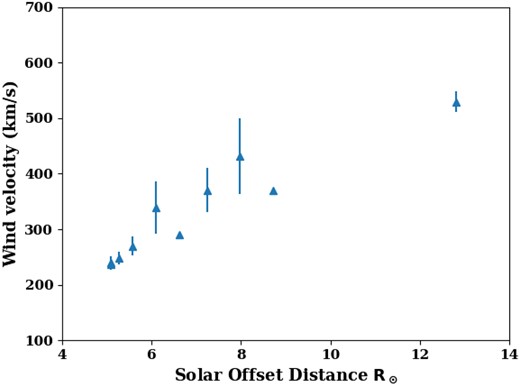
Plasma flow velocities in the inner solar wind derived using quasi-static turbulence formulation from frequency residual data collected at IDSN station.
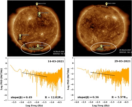
Coronal hole and FF power density spectrum on the given experiment days. Upper panel shows the coronal holes imaged on solar surface by the SDO/AIA spacecraft. Lower panel shows the corresponding power density spectrum of frequency fluctuations, heliocentric distances, and slope. It can be observed that though at separate heliocentric distances the slope values are nearly identical, this is the consequence of the proximate point of our ray path being embedded in the region of influence of solar wind emanating from coronal holes.
Fig. 6 (upper panel) shows the presence of a coronal hole SPoCA 33639 in the SDO/AIA images during the observation period on the two observation days. The turbulence spectrum in Fig. 6 (lower panel) on those days corresponds to two different solar offset distances (on 2021 March 14, it was 12.80 R⊙) and (on 2021 March 29, it was 5.57 R⊙). The slope here represents the 'beta' index value, which corresponds to the linear fit on the log–log curve of turbulence power spectrum (= 2*αf and defined in equation 8 of Section 4.2). On both days, despite being at separate heliocentric distances, the slope is nearly identical (contrary to the expected steepness at larger distances). This interesting aspect of our observation is attributed to the presence of a coronal hole. The coronal holes are the region of open magnetic field lines which aids in the acceleration of the charged particles along them thus leading to the high-speed solar wind. The corroboration of EUV images further reinforces our observation of flatter turbulence spectrum and occurrence of high-speed flow as observed in the results of our solar wind speed models.
5 CONCLUSIONS
We used the coronal radio-sounding experiments, conducted in the inner heliosphere by the Akatsuki spacecraft, to study the characteristics of plasma turbulence and flow speeds. The radio signal obtained at the ground stations was spectrally analysed to find the Doppler residual values. The turbulence spectrum showed the presence of an extended flatter source regime along the entire range of heliocentric distances. We estimated the flow speed of the turbulent plasma in the proximate ray path (the closest path of the radio waves to the solar surface) using the quasi-static turbulence model which is based on the estimation of flow velocities by assuming the propagation of radio waves in turbulent plasma medium where irregularities are assumed to be frozen-in and are advected with the background solar wind speeds. The flow speeds in the inner coronal regions between 5 and 13 R⊙ are estimated as |$220\!-\!550\, \mathrm{km\, s}^{-1}$|. The SDO/AIA coronal images showed the presence of a large coronal hole, which explains the flatter slopes in the turbulence spectrum even with the increasing heliocentric distances and relatively higher flow speeds.
The inner solar coronal region is the main source of solar wind generation and acceleration. However, due to the constraints and paucity of in situ measurements, it has remained a least explored region in the coronal studies. Recent observations from the Parker probe (Kasper et al. 2021; Telloni et al. 2021; Bandyopadhyay et al. 2022; Zhao et al. 2022a, b) and Solar Orbiter (Antonucci et al. 2020; Adhikari et al. 2022) have provided promising insights into these studies, but remote sensing experiments which can transmit signals through these closer heliocentric distances are still one of the ingenious and convenient ways to explore the plasma properties and processes prevailing in this region.
The congruence of the flatter turbulence spectrum, higher flow speeds, and the presence of a coronal hole made this study interesting. This analysis aims at strengthening the observational evidence of turbulence regime and flow speeds present in the least probed inner coronal region.
ACKNOWLEDGEMENTS
We acknowledge the efforts of the ground station team at IDSN, Bangalore India, and UDSC, Japan to track Akatsuki signals. Thanks are also due to Himanshu Pandey and other staff at ISSDC for the proper archival and dissemination of data for further analysis. Special thanks to Soumyaneal, Arya and Ajay of InSWIM lab for their help in error calculations. AB was supported by the Department of Space, India and he was also a JC Bose National Fellow during the period of this work.
DATA AVAILABILITY
The Akatsuki solar radio occultation data are available in JAXA’s data archive Murakami et al. (2017) at https://darts.isas.jaxa.jp/planet/project/akatsuki/rs.html.en.
