


ABSTRACT
We present the first statistical study of spatially integrated non-Gaussian stellar kinematics spanning 7 Gyr in cosmic time. We use deep, rest-frame optical spectroscopy of massive galaxies (stellar mass |$M_\star \gt 10^{10.5} \, \mathrm{M_\odot }$|) at redshifts z = 0.05, 0.3, and 0.8 from the SAMI, MAGPI, and LEGA-C surveys, to measure the excess kurtosis h4 of the stellar velocity distribution, the latter parametrized as a Gauss–Hermite series. We find that at all redshifts where we have large enough samples, h4 anticorrelates with the ratio between rotation and dispersion, highlighting the physical connection between these two kinematic observables. In addition, and independently from the anticorrelation with rotation-to-dispersion ratio, we also find a correlation between h4 and M⋆, potentially connected to the assembly history of galaxies. In contrast, after controlling for mass, we find no evidence of independent correlation between h4 and aperture velocity dispersion or galaxy size. These results hold for both star-forming and quiescent galaxies. For quiescent galaxies, h4 also correlates with projected shape, even after controlling for the rotation-to-dispersion ratio. At any given redshift, star-forming galaxies have lower h4 compared to quiescent galaxies, highlighting the link between kinematic structure and star-forming activity.
1 INTRODUCTION
Galaxies form stars in a fairly regular manner, with their star formation rate (SFR) proportional to their stellar mass (Brinchmann et al. 2004; Noeske et al. 2007). Below this ‘star-forming sequence’ lies a continuous distribution of galaxies with lower (or undetected Feldmann 2017; Eales et al. 2018) SFR. The star-forming sequence thus enables us to divide galaxies between ‘star-forming’ and ‘quiescent’, a classification that maps on to other physical properties of galaxies. If we consider galaxies at or above |$10^{10} \, \mathrm{M_\odot }\,$|,1 star-forming galaxies have flatter intrinsic shapes (Sandage, Freeman & Stokes 1970; Lambas, Maddox & Loveday 1992), less-concentrated light profiles (e.g. Driver et al. 2006; Simard et al. 2011; Bell et al. 2012; Kelvin et al. 2012; Mendel et al. 2014), lower bulge fractions (e.g. Cameron et al. 2009; Simard et al. 2011; Bluck et al. 2014; Mendel et al. 2014), lower velocity dispersion (e.g. Bell et al. 2012; Bluck et al. 2016; Falcón-Barroso et al. 2019), and higher rotation-to-dispersion ratios (V/σ; e.g. Graham et al. 2018; van de Sande et al. 2018; Falcón-Barroso et al. 2019). The overlap between star formation status and other galaxy properties gives us clues on what drives galaxy quenching. For example, the fact that quiescent galaxies have larger bulge mass and higher stellar velocity dispersion has been interpreted as evidence for quenching due to feedback from supermassive black holes (Bluck et al. 2022; Brownson et al. 2022; Piotrowska et al. 2022).
Kinematically, star-forming galaxies have larger V/σ, but otherwise form a continuous distribution with quiescent galaxies, most of which (60–80 per cent, Cappellari et al. 2011; van de Sande et al. 2017a) are also ‘fast rotators’ (Cappellari et al. 2007; Emsellem et al. 2007), albeit with lower average V/σ. At the high-mass end of the quiescent population, we find a distinct kinematic family of ‘slow rotators’ (Brough et al. 2007; Emsellem et al. 2011; Graham et al. 2018; van de Sande et al. 2021a), characterized by round or triaxial intrinsic shapes and no net rotation.
These classifications rely primarily on modelling the stellar velocity distribution as a Gaussian, completely specified by its first three moments.2 However, stellar velocity distributions are known to deviate from a Gaussian (Bender 1990; Rix & White 1992). These deviations contain information about the assembly history of galaxies (Naab et al. 2014); they can be measured by parametrizing the velocity distribution as a Gauss–Hermite series (Gerhard 1993; van der Marel & Franx 1993); the Gauss–Hermite coefficients effectively measure the higher order moments of the distribution. The coefficient of the fourth-order term of the Hermite polynomial, h4, is related to the excess kurtosis of the velocity distribution: |$h_4\, \gt 0$| indicates a leptokurtic distribution (with broader wings compared to a Gaussian), while |$h_4\, \lt 0$| corresponds to a platykurtic distribution (with less prominent wings). Physically, positive h4 is associated with radial anisotropy, which causes a lack of stars near the local circular velocity (e.g. Gerhard 1993). Given that in situ star formation occurs predominantly in discs, radial anisotropy is linked to gas-poor mergers and ex situ stars, and should provide insight on the assembly history of a galaxy, at least up until the last major merger (which may erase the previous kinematic record, Lynden-Bell 1967). van de Sande et al. (2017b) have used spatially resolved higher order kinematics from the SAMI Galaxy Survey (Croom et al. 2012) to investigate the assembly history of nearby galaxies and to match it to the predictions of numerical simulations (Naab et al. 2014). However, h4 also contains information about other kinematic structures, like bars (Seidel et al. 2015; Li et al. 2018), including peanut-shaped bulges (Debattista et al. 2005; Méndez-Abreu et al. 2008), so the physical interpretation of the results is not straightforward.
Because measurements of h4 require higher signal-to-noise data, until now they have been restricted to relatively nearby galaxies (z ≲ 0.1, e.g. Emsellem et al. 2007; van de Sande et al. 2017b). However, new large, ultra-deep spectroscopy surveys enable us, for the first time, to extend these measurements to larger look-back times.
In this work, we use high-quality optical spectroscopy from the local SAMI Galaxy Survey, from the MAGPI Survey (Foster et al. 2021, redshift z = 0.3), and from the LEGA-C Survey (van der Wel et al. 2014, z = 0.8) to investigate the link between star-forming status and higher order kinematics. We start by showing the relation between spatially resolved h4 and the value integrated inside an aperture (Section 2). We then introduce the data (Section 3) and the sample (Section 4). In Section 5, we show that h4 correlates primarily with V/σ and stellar mass; in addition, we also find that at any redshift, star-forming galaxies have lower h4 than quiescent galaxies. We conclude this work with a discussion (Section 6) and with a summary of our findings (Section 7).
Throughout this article, we assume a flat Λ cold dark matter cosmology with |$H_0 = 70 \,\, \mathrm{km\, s^{-1}}\, \, \mathrm{Mpc}^{-1}$| and Ωm = 0.3. All stellar mass measurements assume a Chabrier initial mass function (Chabrier 2003).
2 LOCAL VERSUS INTEGRATED MEASUREMENTS
Given the signal-to-noise ratio (S/N) of some of our data (see Section 3), we propose to obtain only integrated h4, measured from adding the light inside a given aperture. To understand the relation between this measurement of h4 and the local, spatially resolved value used in the literature, we use a toy kinematic model. The model consists of a thin-disc with arctan velocity field, uniform velocity dispersion, and an exponential light profile.3 The velocity field has root-mean square velocity vrms = 300 |$\mathrm{km\, s^{-1}}$| and uniform value of the spatially resolved h4, which we call h4(local), as opposed to h4(integrated). We create a grid by varying the rotation-to-dispersion ratio (V/σ)e (calculated at one effective radius Re 4) and apparent axis ratio q, then add the stellar continuum using the C3K/MIST library (Choi et al. 2016; Conroy et al. 2019), convolved with the appropriate line-of-sight velocity distribution (LOSVD) at each spaxel. From these mock data cubes, we extract the 1D spectrum from an elliptical aperture centred at one Re, as we did for SAMI (see Section 3.1.1). We then measure the integrated h4 using ppxf, the penalized pixel fitting algorithm of Cappellari (2017, 2022). We created seven grids of models, corresponding to seven values of the input, |$h_4\, (\mathrm{local})$|: −0.03, −0.015, 0, 0.015, 0.03, 0.045, and 0.06. These values are chosen to span the range of values we measure in real data (Section 5).
The results are shown in Fig. 1, where the colour and contour lines show the value of the spatially integrated h4 – what we measure for real data in Section 3 – as a function of the model (V/σ)e and q (on the top axis, we also show the model inclination inc). The two panels differ by the input value of the local h4 : 0 for panel a and 0.06 for panel b. It is clear that integrated h4 does not trace only the local h4, but conflates together information from inc and (V/σ)e too. At the same time, the fact that the two figures have largely different colours shows that local h4 is reflected in the value of integrated h4 . In the figures, the locus where integrated and local h4 are the same is traced by the thick, solid line; below this line, integrated h4 tends to be marginally larger than local h4, but well within the observational measurements (which we limit to be |$u(h_4\,) \lt 0.05$|, see Section 4.2). Above the line, integrated h4 reflects primarily (V/σ)e and inclination.
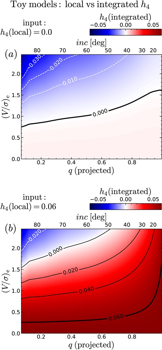
Spatially integrated h4 as a function of (V/σ)e and q for our toy models. Panel a shows the model with local (input) |$h_4\, = 0$|; panel b shows the model with local |$h_4\, = 0.06$|. The dashed/solid contours show loci of constant negative/non-negative |$h_4\, \, (\mathrm{integrated})$|; the thick solid line is the locus where |$h_4\, \, (\mathrm{integrated}) = h_4\, \, (\mathrm{local})$|. For round shapes and/or low (V/σ)e, |$h_4\, \, (\mathrm{integrated})$| reflects |$h_4\, \, (\mathrm{local})$|; elsewhere, |$h_4\, \, (\mathrm{integrated})$| also depends on q and (V/σ)e ; these trends are quantified in Fig. 2 and Table 1; see Fig. 9 for a comparison to the observations (but note that – in our observations – |$h_4\, \, (\mathrm{local})$| is unknown).
In Fig. 2, we consider all seven models, collapsing the grid of (V/σ)e and inc: at any value of |$h_4\, \, (\mathrm{local})$|, the grey circle (and errorbars) represent the median (and 16–84th percentiles) of the measured |$h_4\, \,\, (\mathrm{integrated})$|. If we consider only models with modest rotation support (|$(V/\sigma)_\mathrm{e}\, \lt 0.5$|; blue squares), integrated h4 reflects local h4 with high fidelity (Table 1, row 2; the squares in Fig. 2 have been offset horizontally for clarity). Similar considerations apply to a selection based on apparent axis ratio q: rounder models (q ≥ 0.75; red diamonds) show a tighter relation than the rest of the models (see also Table 1, row 4).
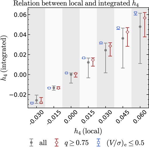
Statistically, |$h_4\, \, (\mathrm{integrated})$| reflects |$h_4\, \, (\mathrm{local})$|, as traced by the grey circles, which are the median values of |$h_4\, \, (\mathrm{integrated})$| over the (V/σ)e –inc grid. Selecting models with large q or low (V/σ)e reduces both the bias and the spread (red diamonds and blue squares, respectively; points inside the same shaded regions have the same local h4: the symbols are offset horizontally for clarity).
Toy-model predictions for the correlations of integrated h4 with each of axis ratio q, rotation-to-dispersion ratio (V/σ)e, and spatially resolved h4. Selecting round galaxies (q ≥ 0.75) or galaxies with low (V/σ)e enhances the correlation between integrated and resolved h4 .
| Subset | q | (V/σ)e | |$h_4 \, (\mathrm{local})$| | |
|---|---|---|---|---|
| (1) | (2) | (3) | (4) | (5) |
| (1) | all | 0.26 | −0.51 | 0.68 |
| (2) | (V/σ)e ≤ 0.5 | 0.12 | −0.12 | 0.98 |
| (3) | (V/σ)e > 0.5 | 0.33 | −0.49 | 0.63 |
| (4) | q ≥ 0.75 | 0.18 | −0.30 | 0.91 |
| (5) | q < 0.75 | 0.08 | −0.74 | 0.54 |
Note. Columns: (1) row index (2) subset of the models used; (3) Spearman’s rank correlation coefficient ρ between integrated h4 and q; (4) same as (3), but for (V/σ)e ; (5) same as (3), but for spatially resolved h4 .
We quantify these correlations using the Spearman’s rank correlation coefficient ρ (Table 1; all correlations are statistically significant). While integrated h4 correlates with all three of q, (V/σ)e, and local h4 (row 1), selecting galaxies with low (V/σ)e (row 2) or round galaxies (row 4) reduces the correlations with q and (V/σ)e (columns 3–4), while bringing the correlation with local h4 to ρ > 0.9 (column 5).
These models are only toy models, to help guide the interpretation of our measurements. In particular, they do not capture the kinematics of intrinsically round, dispersion-supported galaxies (e.g. slow-rotator galaxies, Cappellari et al. 2007; Emsellem et al. 2007). It is clear, however, that for such systems rotation cannot bias h4, because there is little or no rotation to start with. Based on Fig. 2, we expect integrated h4 to correlate with q and to anticorrelate with (V/σ)e . However, if we select round and/or low-(V/σ)e galaxies, integrated h4 reflects the local value, which in turn is related to radial anisotropy (Gerhard 1993; van der Marel & Franx 1993). In the rest of this article, we generally refer to integrated h4 simply as ‘h4 ’, but we will occasionally use ‘integrated h4 ’ when spatially resolved h4 is also relevant.
3 DATA
In this section, we start by presenting the data (Section 3.1), which we draw from three different surveys: the local SAMI Galaxy Survey (z ≈ 0, Section 3.1.1), the MAGPI survey (z ≈ 0.3, Section 3.1.2), and the LEGA-C survey (redshift z ≈ 0.7, Section 3.1.3). Even though data from these three surveys are not homogeneous, we only compare our measurements within surveys, not across surveys – the latter is the subject of a future work. We then explain how the one-dimensional (1D) spectra are used to measure h4 (Section 3.2). Finally, in Section 3.3, we describe ancillary measurements obtained from the literature.
3.1 Data sources
3.1.1 The SAMI Galaxy Survey
The SAMI Galaxy Survey (hereafter simply: SAMI) is a large, optical Integral Field Spectroscopy Survey of local galaxies (0.04 < z < 0.095), covering a broad range of stellar masses (|$10^7 \, \mathrm{M_\odot }\, \lt M_\star \, \lt 10^{12} \, \mathrm{M_\odot }\,$|), morphologies, and environments (local environment density |$0.1 \, \mathrm{Mpc^{-2}} \lt \Sigma _5 \lt 100 \, \mathrm{Mpc^{-2}}$|; Bryant et al. 2015; Owers et al. 2017). SAMI galaxies were observed with the Sydney-AAO Multi-object Integral field spectroscopy instrument (hereafter, the SAMI instrument; Croom et al. 2012), formerly placed at the prime focus of the 4-m Anglo-Australian Telescope. The SAMI instrument has 13 integral field units (IFUs), deployable inside a 1-deg diameter field of view (as well as 26 individual fibres used to sample the sky background). Each of the 13 IFUs is a lightly fused fibre bundle (hexabundle; Bland-Hawthorn et al. 2011; Bryant et al. 2014), consisting of 61 1.6-arcsec diameter individual fibres, for a total IFU diameter of 15 arcsec. The fibres are fed to the double-beam AAOmega spectrograph (Sharp et al. 2006), configured with the 570V grating at 3750–5750 Å (blue arm) and with the R1000 grating at 6300–7400 Å (red arm). With this set-up, the resulting spectral resolutions are R = 1812 (σ = 70.3 |$\mathrm{km\, s^{-1}}$|) and R = 4263 (σ = 29.9 |$\mathrm{km\, s^{-1}}$|) for the blue and red arm, respectively (van de Sande et al. 2017b). Each galaxy was exposed for approximately 3.5 h, following a hexagonal dither pattern of seven equal-length exposures (Sharp et al. 2015). After rejecting observations under inadequate conditions, the median full width at half-maximum (FWHM) seeing of the SAMI data cubes is 2.06 ± 0.40 arcsec. The data reduction is described in Sharp et al. (2015) and Allen et al. (2015), whereas subsequent improvements have been described in the public data release papers (Green et al. 2018; Scott et al. 2018). In this work, we use data from the third and final public data release (Data Release 3, hereafter DR3) consisting of 3068 unique data cubes (Croom et al. 2021a). For our measurements, we use 1D spectra obtained by adding the light inside an elliptical aperture. The ellipse is centred on the centre of the galaxy, its position angle and shape are taken from the best-fitting Sérsic model, and its semimajor axis is equal to one effective radius Re (see Section 3.3.2 for the size and shape measurements). The median S/N of these spectra is 24 Å−1. Two randomly selected SAMI spectra are shown in Fig. 3, illustrating a quiescent galaxy (SAMI 347471, panel a) and a star-forming galaxy (SAMI 517278, panel d). The galaxy images (obtained from the data cubes) and the elliptical apertures are illustrated in panels c and f. Note that the SAMI wavelength range has been reduced to match the wavelength range of LEGA-C. The reason is that we find h4 to depend on the wavelength range, which we will explore in a future paper (D’Eugenio et al. 2023).
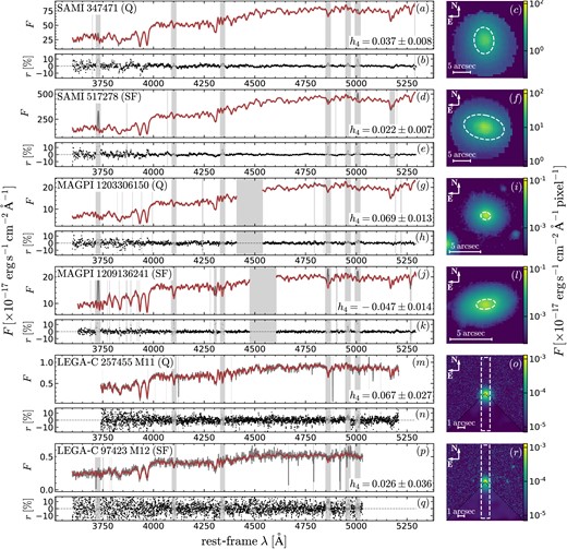
Comparison between three randomly selected quiescent (Q) galaxies and three randomly selected star-forming (SF) galaxies, chosen from SAMI (panels a–f), MAGPI (panels g–l), and LEGA-C (panels m–r). For each galaxy, we show the data (dark grey) and best-fitting spectra (red), alongside the relative residuals (black dots). The galaxy names and their h4 values are reported in the top-left and bottom-right corners of the panels with the spectra. The vertical lines/regions are masked because of low data quality, or possible emission lines (regardless of whether lines were actually detected), or because of instrument set-up (e.g. the GALACSI laser band for MAGPI, panels g, h, j, and k). The inset figures show the galaxy images (derived from the data cubes for SAMI and MAGPI, panels c, f, i, and l; from HST F814W for LEGA-C, panels o and r). In each of the six galaxy images, we indicate the aperture used to extract the spectrum with a dashed white line; these are ellipses with semimajor axis equal to the effective radius (for SAMI and MAGPI), or a rectangular slit with 1-arcsec width (for LEGA-C). The lowest quadrant of the LEGA-C images shows the data convolved to the ground-based spatial resolution of LEGA-C.
3.1.2 MAGPI
The Middle Ages Galaxy Properties with Integral Field Spectroscopy survey (hereafter, MAGPI; Foster et al. 2021) is a Large Program with the Multi-Unit Spectroscopic Explorer (MUSE, Bacon et al. 2010) on the European Southern Observatory (ESO) Very Large Telescope (VLT). MAGPI targets spatially resolved galaxy physics in redshifts 0.15 < z < 0.6, the uncharted cosmic ‘Middle Ages’ between ‘classic’ local surveys (e.g. SAMI) and LEGA-C. The sample consists of 60 central galaxies: 56 drawn from the Galaxy and Mass Assembly survey (GAMA; Driver et al. 2011; Liske et al. 2015; Baldry et al. 2018), complemented by four fields chosen from two legacy programs, targeting clusters Abell 370 (Program ID 096.A-0710; PI: Bauer) and Abell 2744 (Program IDs: 095.A-0181 and 096.A-0496; PI: Richard). In addition to the central galaxies, MAGPI will concurrently observe 100 satellite galaxies in the target redshift range, plus any background galaxy inside the MUSE field of view.
MAGPI uses MUSE in the large-field configuration (1 × 1-arcmin2 field of view), aided by Ground Layer Adaptive Optics GALACSI (Arsenault et al. 2008; Ströbele et al. 2012) to achieve a spatial resolution with median FWHM of 0.6–0.8 arcsec (comparable, in physical units, to the spatial resolution of local surveys such as SAMI). MUSE spectra cover the approximate rest-frame wavelength range 3600 Å < λ < 7200 Å, with a median spectral resolution FWHM of 1.25 Å (inside one effective radius, the FWHM varies by 3 per cent). The survey is ongoing, but the program has already obtained fully reduced data for 35 fields, though in this work we use only the first 15. An overview of the observations and data reduction is provided in the survey paper (Foster et al. 2021), while the full data reduction pipeline (based on the MUSE pipeline, Weilbacher et al. 2020 and on the Zurich Atmosphere Purge sky-subtraction software, Soto et al. 2016) will be described in an upcoming work (Mendel et al., in preparation). Each MAGPI cube is segmented into ‘minicubes’, centred on individual galaxy detections. From these minicubes, we obtain 1D spectra by adding up the light inside an aperture, similar to the approach we used for SAMI. These spectra have median S/N = 13 Å−1, but the subset we use in this study has larger S/N (see Section 4.2). Two randomly selected MAGPI galaxies are shown in Fig. 3: quiescent MAGPI 1203306150 (panels g–i) and star-forming MAGPI 1209136241 (panel j–l). Like for SAMI, the wavelength range has been reduced to match the wavelength range of LEGA-C.
3.1.3 LEGA-C
The Large Early Galaxy Astrophysics Census is the deepest, large spectroscopy survey beyond the local Universe (van der Wel et al. 2016). Targeting 3000 galaxies in the range 0.6 < z < 1.0, LEGA-C delivers high-quality absorption spectra at a look-back time when the Universe was only half its age. The sample is Ks-band selected from the UltraVISTA catalogue (Muzzin et al. 2013a), itself part of the COSMOS field, thus (mostly) covered by the COSMOS HST survey (Scoville et al. 2007). LEGA-C spectra were observed at the ESO VLT using the now decommissioned VIMOS spectrograph (Le Fèvre et al. 2003) in its multi-object configuration, with mask-cut slits of 1-arcsec width and length ≥8 arcsec. All slits from the main survey were oriented in the north–south direction, therefore randomly aligned with respect to the major axes of the targets. The seeing median FWHM (measured from a Moffat fit on the slit data) is 0.75 arcsec (van Houdt et al. 2021). The spectral interval varies with the slit position within the relevant mask (but typically covers the interval 6300 Å < λ < 8800 Å), with an observed-frame spectral resolution R = 2500 (the effective spectral resolution is R = 3500, because the LEGA-C targets underfill the slit; Straatman et al. 2018). Each target was exposed for 20 h, reaching an integrated continuum S/N ≈ 20 Å−1. Given the depth of the observations, most targets have successful kinematics measurements (93 per cent) resulting in a mass-completeness limit of |$10^{10.5} \, \mathrm{M_\odot }\,$| (van der Wel et al. 2021).
To measure h4, we use the 1D LEGA-C spectra from the third public data release of LEGA-C (DR3, van der Wel et al. 2021). These were obtained from optimal extraction (Horne 1986) of the 2D spectra. The large physical width of the LEGA-C slits (7.5 kpc at z = 0.8) means that the 1D spectra sample a representative fraction of the targets’ light (the ratio between the slit width and the circularized galaxy diameter is 1.2 ± 0.8 for our sample, see Section 4 for the sample selection). We adopt the method described in Section 3.2, setting the (observed-frame) FWHM to a wavelength-independent value of 2.12 Å (corresponding to 86 |$\mathrm{km\, s^{-1}}$|, van der Wel et al. 2021). Note that we use emission-line-subtracted spectra (Bezanson et al. 2018), but the precision and accuracy of the subtraction do not affect our measured kinematics. This is because we conservatively mask the spectral regions where gas emission lines may arise in all galaxies, regardless of whether emission was actually detected (see Section 3.2 and Appendix A). Two randomly selected LEGA-C spectra are shown in Fig. 3: a quiescent galaxy (LEGA-C 257455 M11, panel m) and a star-forming galaxy (LEGA-C 97423 M12, panel p). The HST images and the LEGA-C slits are shown in panels o and r.
3.2 Measuring integrated higher order kinematics
In each of the three data sets, we model the LOSVD as a fourth-order Gauss–Hermite series (Gerhard 1993; van der Marel & Franx 1993), because this approach: (i) provides a compact description of the non-Gaussianity through the parameters h3 and h4, the coefficients of the third- and fourth-order Hermite polynomials, as well as (ii) minimizes the correlation between the LOSVD parameters (van der Marel & Franx 1993).
Our h4 measurements are based on one-dimensional spectra spanning rest-frame B and g band, from which we infer the LOSVD using ppxf. We model the spectra using a linear combination of simple stellar population (SSP) spectra from the MILES library (Vazdekis et al. 2010, 2015), using BaSTI isochrones (Pietrinferni et al. 2004, 2006) and solar [α/Fe].
When necessary and possible, the SSP spectra are matched to the spectral resolution of the data, using the uniform FWHM spectral resolution of 2.51 Å (Falcón-Barroso et al. 2011). However, for some of the SAMI spectra, and for all the MAGPI and LEGA-C spectra, the instrumental resolution is better than the MILES spectral resolution. In this case, matching the two resolutions would require broadening the galaxy spectra, but because this is undesirable, we do not apply any correction. Even though this introduces a bias in the resulting second moment of the LOSVD, the MILES SSP library provides consistently the best fits to the galaxy continuum (surpassed only by the MILES stellar template library, in agreement with e.g. van de Sande et al. 2017b; Maseda et al. 2021). There are three reasons why a biased measurement of the second moment is not important in this article. First, we are not interested in measuring the second moment; when we use second moment measurements, these values are taken from the literature and are measured taking into account the appropriate instrument resolution (Section 3.3). Second, our main targets are high-mass galaxies with large physical dispersion and, finally, our results are unchanged if we repeat our measurements with the higher resolution SSP spectra from the Indo-US library (Valdes et al. 2004), or with the synthetic SSPs from the C3K theoretical library (Conroy et al. 2019) using the MIST isochrones (Choi et al. 2016; Dotter 2016. See Appendix B). Overall, we deem the fit quality a more desirable property than unbiased measurements of the second moment (which are available anyway from other sources). For this reason, our default h4 measurements are obtained using the MILES SSP templates.
In addition to the SSP templates, we also use 12th-order additive Legendre polynomials to fit residual flux due to flux calibration and background subtraction errors (this follows the prescription of D’Eugenio et al. 2020 for LEGA-C, and of van de Sande et al. 2017b for SAMI). The keyword bias, which determines the amount of penalization against non-Gaussian LOSVDs, is set to its default value. This choice does not affect our measurements of h4, because of the high S/N of our spectra (see Section 3.2.1).
The fit is repeated twice: in the first iteration, we use uniform weighting for all valid spectral pixels. After this fit, we rescale the noise spectrum so that the value of the reduced χ2 would be unity. The second and final fit uses this rescaled noise as well as 3|$\sigma$| iterative clipping to remove outliers. ppxf returns the first (non-trivial) four moments of the LOSVD: mean velocity V, σ, h3 (a measure of skewness), and h4 (measuring excess kurtosis).
The uncertainties on the h4 measurements are derived from the local curvature of the χ2 surface near its minimum. We checked that these formal uncertainties accurately propagate the observational errors through to the derived parameter values, using a Monte Carlo (MC) approach. For each galaxy, we created 100 spectra by randomly shuffling and re-adding the fit residuals to the best-fitting spectrum (see e.g. van de Sande et al. 2017b). After fitting these random realizations of the data, for each galaxy we obtain a distribution of 100 values of h4; the MC uncertainty is defined as the standard deviation of this distribution. For SAMI, and for 10 per cent of the LEGA-C sample, these MC uncertainties are consistent with the default uncertainties, so, from here on, we always use the formal uncertainties as default.
Example ppxf fits are shown in Fig. 3; starting from the final sample (defined in Section 4.3), we randomly selected a quiescent and a star-forming galaxy from each of the three surveys. Note the different apparent sizes in the inset images, but the similar wavelength coverage of the spectra.
In Fig. 4, we show two example spectra from SAMI: a galaxy with non-Gaussian, leptokurtic LOSVD (|$h_4\, \gt 0$|, top panel) and a galaxy with (close-to) Gaussian LOSVD (bottom panel). In each panel, we show two spectra: the sand-coloured line is the ratio between the data and the 4-moments best-fitting spectrum, whereas the black line is the ratio between the 4-moments best-fitting spectrum and the Gaussian best-fitting spectrum (vertical grey regions are masked). For galaxy SAMI 23623, the sand and black lines have several features in common, both around the Calcium H and K lines as well as around 4200 Å; in contrast, no such features are present for galaxy SAMI 107135. This figure demonstrates that information about the shape of the LOSVD is spectrally ‘distributed’: it is present both around prominent lines, as well as in less prominent spectral features.
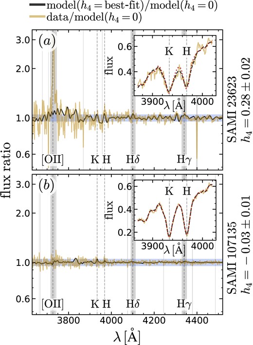
Showing the difference between a second- and fourth-order velocity distribution. In the main panels, the sand lines show the ratio between the data and the best-fitting second-order model (labelled ‘model (h4 = 0)’), whereas the black lines show the ratio between the best-fitting fourth- and second-order models. Panel a shows SAMI galaxy 23623, an extreme system with high h4 (this galaxy appears to be a recent merger, so it is excluded from the rest of the study). For this galaxy, outside the noisy region at the blue end (λ < 3900 Å), the residuals show variations of a few percent (the shaded blue region encompasses ±5 per cent from unity); the solid black line follows closely the sand line, underscoring the need for a leptokurtic LOSVD. Conversely, SAMI galaxy 107135 (panel b) has low h4: the difference between the second- and fourth-order LOSVDs is less pronounced. The vertical grey regions are bad pixels, or regions where gas emission lines may be located. In each of the inset panels, we focus on the region of the spectrum around the H and K Calcium lines; we show the data (solid sand line), the best-fitting fourth-order model (dashed black line) and the best-fitting second-order model (dotted red line). Even for SAMI 23623, the two models are barely distinguishable, but comparing the the fourth- and second-order models in the region between the two lines, it may be observed that the fourth-order model has broader wings, which follow the data more closely.
3.2.1 Penalization of non-Gaussian solutions
To measure h4, a critical feature of the ppxf algorithm is the eponymous ‘penalization’ against non-Gaussian LOSVDs. The penalization is an arbitrary upscaling of the χ2, to ensure non-Gaussian solutions (i.e. hi ≠ 0) are accepted only if they come with a ‘sufficient’ decrease in the χ2 (Cappellari & Emsellem 2004). In ppxf, the penalization is implemented by the bias keyword. To recover h4 in low-quality data, the value of the bias keyword must be carefully determined using simulations (see e.g. van de Sande et al. 2017b, their appendix A.5). For low-S/N spectra, h4 may depend on the choice of bias, but in this work, we deal with high-S/N data, so the value of bias is not critical. To demonstrate this, we re-measured h4 setting bias = 0 and verified that our results do not change. For our sample (defined in Section 4.3), the difference |$\Delta \, h_4\,$| between the ‘non-penalized’ h4 measurement (bias = 0) and the default ‘penalized’ h4 measurement (bias = None) is negligible compared to other systematic errors (which have values of ≈0.03, Appendix C). For SAMI, we find a median |$\Delta \, h_4\, =0.0005\pm 0.0001$|, whereas for LEGA-C we find a median |$\Delta \, h_4\, =0.0002\pm 0.0004$| (for MAGPI, the uncertainty on the median |$\Delta \, h_4\,$| is much larger than the median itself, because of the small sample size). In all three samples, the standard deviations of |$\Delta \, h_4\,$| are 3–10 times smaller than the precision threshold for selecting the sample (see Section 4.2).
3.2.2 Measurement bias
In the following text, we aim to compare h4 between star-forming and quiescent galaxies; this is subject to possible bias due to the systematic differences in the depth of stellar absorption features in these two classes of galaxies: at fixed luminosity (and so at fixed S/N), quiescent galaxies have older stellar populations, so have deeper absorption features (except for Balmer lines, which we mask as we discuss in Section 4.2). Using mock spectra, we find that systematics connected to different stellar populations are ×10 smaller than the maximum measurement uncertainties used for the quality cut, and smaller than the reported difference between star-forming and quiescent galaxies5 (Appendix C).
Similarly, changing the template library used in ppxf changes the value of measured h4, but we still measure a different h4 between star-forming and quiescent galaxies (Appendix B).
3.3 Ancillary data
3.3.1 Stellar masses
Stellar masses are obtained differently for SAMI and MAGPI compared to LEGA-C. For the first two surveys, M⋆ was derived from Sérsic-fit i-band total magnitudes, using g − i colour to infer the stellar mass-to-light ratio, assuming exponentially declining star formation histories (Taylor et al. 2011). The actual expression of stellar mass also implements a k-correction (see e.g. Bryant et al. 2015). For SAMI, g − i colours are derived from SDSS or VST ground-based photometry (see again Bryant et al. 2015; Owers et al. 2017, and references therein). For MAGPI, colours are derived from synthetic MUSE photometry (Taylor et al., in preparation).
In contrast, LEGA-C uses SED fits to observed-frame BVrizYJ photometry drawn from UltraVISTA (Muzzin et al. 2013b), zero-point corrected as described in the DR3 article (van der Wel et al. 2021). The fits are performed using prospector (Leja et al. 2019a; Johnson et al. 2021), with the configuration adopted in Leja et al. (2019b).
All three methods rely primarily on rest-frame visible photometry, but the precise bands and the underlying assumptions about dust, star formation history, and metallicity are different. Despite these differences, however, the mass measurements are sufficiently close for a qualitative selection in M⋆ (see Section 4.3). To prove this statement, we use a third set of mass measurements as a ‘bridge’. These measurements are only available for a subset of the LEGA-C and SAMI surveys, so they are not suitable as main mass measurements. Driver et al. (2018) used magphys (da Cunha, Charlot & Elbaz 2008) to measure stellar masses for the subsets of the SAMI and LEGA-C samples that fall within the footprint of GAMA. The SAMI measurements show good agreement with the default measurements we use here: the median offset between the g − i-based (default) and magphys measurements is 0.01 dex, with a scatter of 0.06 dex. For LEGA-C, the median offset between the prospector (default) and magphys measurements is 0.03 dex, with a scatter of 0.07 dex.
3.3.2 Sizes and shapes
Galaxy sizes and shapes are derived from Sérsic models. Re is defined as the half-light semimajor axis and q is the minor-to-major axis ratio of the best-fitting model. For SAMI, we use ground-based r-band photometry. For MAGPI, we use synthetic r-band imaging obtained from MUSE. For LEGA-C, we use HST F814W images. These heterogeneous data have remarkably similar spatial resolution in physical units; considering a median point-spread function FWHM of 1.3, 0.6, and 0.12 arcsec, respectively, for SAMI, MUSE, and LEGA-C photometry, the spatial resolution in physical units is within a factor of 3 (1.3, 2.7, and 0.9 kpc, respectively).
For SAMI, the models are optimized using either galfit (Peng et al. 2002, for the SAMI subset inside the GAMA regions), or profit (Robotham et al. 2017; for the cluster subset). We refer the reader to the relevant literature for further information (Kelvin et al. 2012; Owers et al. 2019; Croom et al. 2021a). For both MAGPI and LEGA-C, the Sérsic models are optimized using galfit (for LEGA-C, see also van der Wel et al. 2011, 2021).
While the measurements (and especially LEGA-C) are not strictly consistent, we use them only internally to each sample and make no attempt to compare values across surveys. To test the effect of the different rest-frame wavelength of the photometry, we replace SAMI r-band photometry with g-band photometry. This substitution matches well the rest-frame wavelength of LEGA-C (the effective wavelength of the SDSS g filter is 4670 Å; at redshift z = 0.7, the rest-frame effective wavelength of the ACS F814W filter is 4710 Å). Comparing g-band to r-band photometry for the subset of our sample that possess both measurements, we find that the median ratio of g-band to r-band axis ratio is 1.01. The median ratio between the effective radii is 1.04. These small differences are negligible, given the precision of our measurements and our sample size. Nevertheless, we tested that replacing the SAMI r-band sizes and shapes with their g-band equivalents does not change our conclusions. In the end, we prefer to use r-band measurements because g-band sizes and shapes are only available for two-thirds of the SAMI sample.
3.3.3 Rotation-to-dispersion ratio and other kinematic quantities
For SAMI, MAGPI, and LEGA-C, we also use two different measurements of (V/σ)e; for SAMI and MAGPI, this is the observed ratio averaged inside one Re, with empirical corrections for seeing and aperture (van de Sande et al. 2017a, 2021a, b; Harborne et al. 2020); for LEGA-C, (V/σ)e indicates the value of the best-fitting Jeans anisotropic models (Cappellari 2008), evaluated at one Re (the models and their optimization are described in van Houdt et al. 2021). Once again, we remark that these two measurements are not consistent, but we do not compare them directly.
It is worth noting that dynamical models (and therefore (V/σ)e) are only available for approximately one-third of LEGA-C galaxies. This occurs mostly because galaxies where the slit is misaligned compared to the major axis of the galaxy were not modelled (van Houdt et al. 2021). Fortunately, for the mass range considered in this article, the galaxies with available models and (V/σ)e represent a random subset of the parent population. We used a Kolmogorov–Smirnov (KS) test to assess if the mass distribution of our sample is the same as the mass distribution of the subset with dynamical models; we find a probability PKS = 0.8 (for quiescent galaxies) and PKS = 0.6 (for star-forming galaxies). Similar probabilities are found for the distribution of Re. In contrast, comparing the distribution of position angles (which determine the availability of dynamical models) we find PKS = 3 × 10⁻¹³ and PKS = 7 × 10⁻⁵ for quiescent and star-forming galaxies, respectively.
We also use integrated velocity dispersions within a fixed aperture, σap. For SAMI and MAGPI, these are calculated inside the ellipse of semimajor axis equal to one Re; for LEGA-C, these are calculated from the 1D spectrum.
Finally, for SAMI only, we use the visual kinematic classification of van de Sande et al. (2021a) to separate dispersion-supported galaxies from rotation-supported galaxies. We define slow rotators (SR) as having kin_mtype<1, which consists of all ‘non-obvious rotators’ without kinematic features (e.g. no kinematically decoupled cores), plus intermediate systems between this class and non-obvious rotators with features. This definition has good overlap with other definitions of SRs in the literature (van de Sande et al. 2021a).
4 SAMPLE SELECTION
In this section, we aim to present the motivation, selection criteria, and properties of our sample.
We propose to study the difference between star-forming and quiescent galaxies, so the sample is split between these two classes (Section 4.1). To ensure that our measurements are reliable, we introduce a quality selection (Section 4.2), and, finally, we introduce a cut in stellar mass to ensure that our results are representative (Section 4.3).
4.1 Star-forming and quiescent galaxy separation
For SAMI, we use the definition of Croom et al. (2021b): quiescent galaxies have star SFRs more than 1.6 dex below the star-forming sequence as defined in Renzini & Peng (2015). SFRs are taken from the SAMI DR3 catalogue (Croom et al. 2021a) and are measured from the total, dust-corrected H α flux as originally described in Medling et al. (2018).
For MAGPI, we use a mixed approach. For galaxies with z > 0.41, the MUSE spectra do not include H α, so we used an empirical criterion based on the equivalent width (EW) of H β: galaxies with EW(H β) < −1 Å are classified as star-forming (see e.g. Wu et al. 2018), the others are classified as quiescent. For galaxies with z < 0.41, the MUSE wavelength range does include H α. For these targets (the majority of the final sample), we measure the total H α and H β flux inside the circular aperture with radius equal to three Re (after subtracting the continuum, using ppxf). We then apply an attenuation correction assuming an intrinsic H α/H β ratio of 2.86 (case B recombination and |$T_\mathrm{e} = 10^4\, \mathrm{K}$| Osterbrock & Ferland 2006) and the Cardelli, Clayton & Mathis (1989) dust extinction law. SFRs are measured using the Kennicutt (1998) calibration. When no H α emission is detected, we classify the galaxy as quiescent. For galaxies that do have an SFR measurement, we compare our measurements to the values from GAMA, finding six galaxies in common and a root-mean square difference of 0.25 dex. In addition to galaxies with no detected H α emission, or with low-EW H β emission, we also consider quiescent all galaxies that do have a measured SFR, but lie at least 1 dex below the star-forming sequence. As a reference, we use the empirical, redshift-dependent relation of Whitaker et al. (2012).
For LEGA-C, we use only galaxies from the ‘primary’ LEGA-C sample, and adopt the UVJ diagram (Labbé et al. 2005; Straatman et al. 2018) to discriminate star-forming and quiescent galaxies.
The different definitions of star-forming and quiescent galaxies may be a concern, but, in practice, they are largely equivalent. This has been shown explicitly for SAMI and LEGA-C (Barone et al. 2022).
4.2 Quality selection
With the default separation between star-forming and quiescent galaxies, we were able to measure h4 for a parent sample consisting of 2864 SAMI galaxies (out of 3084 in the DR3 sample), 131 MAGPI galaxies (out of 159), and 2525 (out of 2636) LEGA-C galaxies. However, sampling of the galaxy mass function below |$M_\star \, = 10^{10} \, \mathrm{M_\odot }\,$| is highly incomplete, so, in the following text, we consider only galaxies above the aforementioned mass threshold. This sample consists of 1822, 61, and 2475 galaxies for SAMI, MAGPI, and LEGA-C, respectively.
In Fig. 5, we show the relation between the measurement uncertainty about h4, labelled |$u(h_4\,)$|, and the empirical (ppxf-derived) S/N for the three samples, divided between star-forming and quiescent galaxies with the criteria described in Section 4.1. For SAMI and LEGA-C, we represent the data using dashed blue/solid red contours for star-forming and quiescent galaxies, respectively (panels a and c); these contours enclose the 30th, 50th, and 90th percentiles of the sample. For MAGPI, the sample size is considerably smaller, so we use blue diamonds/red circles that represent individual galaxies (panel b). By comparing the locus of star-forming and quiescent galaxies, it is clear that star-forming galaxies have larger |$u(h_4\,)$| than quiescent galaxies at fixed S/N. This is a reasonable outcome, because our ability to constrain h4 depends not only on the continuum S/N, but also on the number and strength of stellar spectral features. These features are typically weaker in star-forming galaxies than in quiescent galaxies6 (see e.g. van der Wel et al. 2021, their fig. 4).
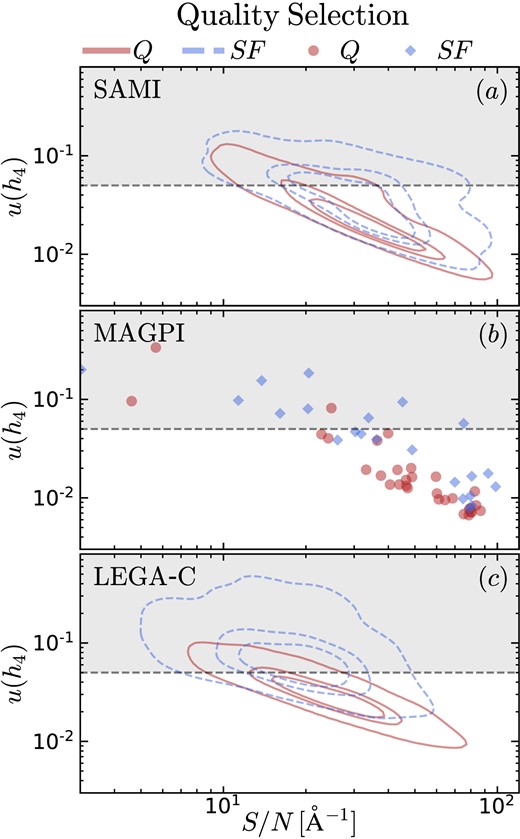
Our quality selection is based on a cut in the h4 measurement uncertainty, |$u(h_4\,)\lt 0.05$| (horizontal dashed line). There is a clear relation between |$u(h_4\,)$| and empirical S/N, for SAMI (panel a), MAGPI (panel b), and LEGA-C (panel c). For SAMI and LEGA-C, we use contour lines enclosing the 30th, 50th, and 90th percentile of the data; dashed blue/solid red contours trace star-forming/quiescent galaxies, respectively. For MAGPI, we represent individual star-forming/quiescent galaxies with blue diamonds/red circles. Note that, at fixed S/N, star-forming galaxies have larger |$u(h_4\,)$| than quiescent galaxies.
Because of the different precision between star-forming and quiescent galaxies of the same S/N, a selection based solely on S/N would mix together high-precision h4 values for one subset of galaxies with low-precision measurements for the other. To avoid this potential bias, we adopt a quality cut at |$u(h_4\,)\lt 0.05$| (horizontal dashed line). With this cut, the median S/N values are 31 ± 16 Å−1 (for SAMI), 45 ± 30 Å−1 (MAGPI), and 20 ± 10 Å−1 (LEGA-C). Admittedly, this cut is arbitrary, but we note that adopting a threshold between 0.02 and 0.1 does not change our results. If we select |$u(h_4\,)\lt 0.01$|, then the LEGA-C sample is too small to infer any trend with redshift (just nine galaxies). Similarly, we tested that a cut in S/N > 30 Å−1 does not change our results.
4.3 Stellar mass selection and completeness
Of the 3083 galaxies in the SAMI DR3 sample, only 1325 meet the quality selection threshold (defined in Section 4.2), giving a completeness of only 43 per cent. Similar survival rates apply to MAGPI and LEGA-C (27 per cent and 45 per cent, respectively). To avoid sample incompleteness caused by the quality selection, we require galaxies in our sample to have |$M_\star \, \gt 10^{10.5}\, \mathrm{M_\odot }\,$| (cf. hatched regions in Fig. 6). The sample is thus defined as all galaxies with |$M_\star \, \gt 10^{10.5} \, \mathrm{M_\odot }\,$| and |$u(h_4\,)\lt 0.05$|. This particular mass threshold was chosen as a compromise between sample size and completeness.
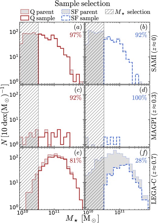
The sample selected from SAMI (top row), MAGPI (middle), and LEGA-C (bottom). The left/right columns show, respectively, quiescent and star-forming galaxies. In each panel, the filled grey histogram is the mass distribution of the parent sample (including galaxies without h4 measurements). The empty histograms are our sample, selected to have |$M_\star \, \ge 10^{10.5}\, \mathrm{M_\odot }\,$| and to meet the quality selection criteria for h4 (Section 4.2). The percentage in the top right corner of each panel is the number ratio between our sample and the parent sample, considering only galaxies above the mass limit. For SAMI and LEGA-C, the quiescent samples are highly complete; for the star-forming sample, only SAMI shows high completeness.
In the top row of Fig. 6 we compare the mass distribution of the SAMI parent sample to that of our sample, separately between quiescent (panel a) and star-forming galaxies (panel b). Above the mass threshold of |$10^{10.5} \, \mathrm{M_\odot }\,$|, the SAMI DR3 sample contains 821 unique galaxies, of which 780 meet the quality selection criteria (95 percent). Considering separately quiescent galaxies, the SAMI DR3 sample and our sample consist of 481 and 465 galaxies (97 percent, cf. grey filled and red empty histograms in panel a); for star-forming galaxies, the numbers are 340 and 315 (92 percent, cf. grey filled and blue empty histograms in panel b).
In the second row of Fig. 6, we provide the mass distribution for the MAGPI sample. Above the adopted M⋆ limit, we have 32 galaxies, of which all but two pass the quality selection (92 per cent). Separating between quiescent and star-forming galaxies (panels c and d), we have similar completeness values (22/24 quiescent galaxies and 8/8 star-forming galaxies meet the quality selection criteria).
Finally, in the bottom row of Fig. 6, we compare the mass distribution of the LEGA-C parent sample to that of our final sample, divided again between quiescent (panel e) and star-forming galaxies (panel f). For quiescent galaxies, the LEGA-C primary sample consists of 1005 galaxies with |$M_\star \, \gt 10^{10.5} \, \mathrm{M_\odot }\,$| and the LEGA-C final sample consists of 818 galaxies (81 percent, cf. grey filled and red empty histograms in panel e). For star-forming galaxies, the numbers are 1210 and 339 (28 percent, cf. grey filled and blue empty histograms in panel f).
Thus, in summary, our sample provides a highly complete view of the SAMI galaxies and of the LEGA-C quiescent galaxies, but is considerably skewed to large M⋆ for the LEGA-C star-forming subset. For MAGPI, our selection is highly representative of the parent sample, but the parent sample is itself skewed to large values of M⋆, because MAGPI focuses on central galaxies. Given that we find h4 to correlate with M⋆, correcting for the selection bias against low-mass star-forming galaxies in LEGA-C leads to our results becoming even stronger (cf. Appendix D).
Note that when we compare h4 to other galaxy observables in Sections 5.3–5.5, the actual sample sizes vary according to the availability of the ancillary data required for each comparison. In most cases, the change in sample size is small (e.g. only 454/507 quiescent SAMI galaxies have measurements of (V/σ)e). However, we stress again that only one-third of LEGA-C galaxies have measurements of (V/σ)e (i.e. only 297/818 quiescent galaxies and only 132/339 star-forming galaxies), but this selection causes no bias, as it is a selection by position angle only.
5 RESULTS
In this section, we show that star-forming and quiescent galaxies have different distributions of h4, even after matching the samples by stellar mass or S/N (Section 5.1). We then investigate the relation of h4 with (V/σ)e and q (Section 5.2) and find the trends expected from the toy model of Section 2. We then move on to study what other galaxy observables are good predictors of h4, starting with stellar mass and size (Section 5.3), stellar mass, and aperture dispersion (Section 5.4), and, finally, stellar mass and rotation-to-dispersion ratio (Section 5.5), which we find to be the two most likely drivers of h4.
Throughout this section, we use two statistical tools. To compare the distribution of h4 between star-forming and quiescent galaxies (Section 5.1) we use the KS test, for which we quote only the probability value PKS.
In Sections 5.2 and 5.3–5.5, we study how h4 varies as a function of two other observables. In all cases, these two observables are correlated (e.g. the mass–size relation, Section 5.3, or the stellar-mass Faber–Jackson relation, Section 5.4). As a means to distinguish between primary correlations among related variables, and secondary correlations that arise as a consequence of primary correlations, we use partial correlation coefficients (PCCs; see e.g. Bait, Barway & Wadadekar 2017; Bluck et al. 2019; Baker et al. 2022). In general, if two variables x and z (e.g. M⋆ and h4) are both independently correlated with a third variable y (e.g. Re), then this will induce an apparent correlation between y and z (i.e. h4 and Re). PCCs address this issue by quantifying the strength and significance of the correlation between y and z, while controlling for x. Similar to the standard Spearman rank correlation coefficient, a value of zero implies no correlation, and −/+1 implies perfect anti/correlation. In the following text, we denote with |$\rho (x, z \vert \, y)$| the PCC between x and z removing the effect of y. In the context of PCCs, P is the probability that the measured PCC arose by chance from uncorrelated data. In the relevant figures, we also provide the graphical representation of the PCCs as an arrow; the angle and direction of this arrow are defined by the |$\arctan$| of the ratio between the PCCs (Bluck et al. 2020a). On the x–y plane, an angle equal to 0° means that z correlates with x but not y; 90° means that z correlates with y but not x, 180° means that z anticorrelates with x but not with y, and so on. Note that, in principle, a meaningful arrow representation requires that the figures are scaled so that the data have the same standard deviation along x and y. Because this is not always practical (i.e. to avoid figures with unsavoury aspect ratios), the arrows are always scaled as if the data have the same standard deviation, even when the figures are not.
5.1 Different h4 between star-forming and quiescent galaxies
Fig. 7 shows h4 for star-forming (SF, blue) and quiescent galaxies (Q, red), as a function of M⋆ and S/N. The first two columns show the SAMI sample (panels a–e) and the last two columns show the LEGA-C sample (panels f–j); the MAGPI sample is not shown in this figure. The blue circles/red diamonds represent individual star-forming/quiescent galaxies.
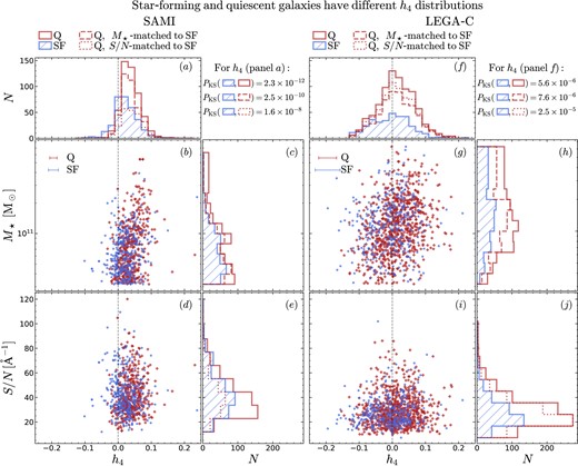
On average, quiescent (Q) galaxies have larger h4 compared to star-forming (SF) galaxies, even after controlling for stellar mass or S/N. Panels a–e show SAMI galaxies, panels f–j show LEGA-C galaxies. In panels b, d, g, and i, the blue circles/red diamonds represent star-forming/quiescent galaxies; the errorbars are the median uncertainties (for h4) or a uniform uncertainty of 0.15 dex (for M⋆). All other panels show the marginalized distributions. The vertical dashed lines trace |$h_4\, = 0$|, corresponding to a Gaussian LOSVD. Star-forming and quiescent galaxies have different h4 distributions (hatched blue and red histograms in panels a and f), but could this difference be due to different M⋆ or S/N distributions? (cf. panels b, d, g, and i). The dashed red histograms show a sample of quiescent galaxies randomly drawn to match the M⋆ distribution of the star-forming sample (for SAMI: panels a and c, for LEGA-C: panels f and h); the dotted red histograms show a sample of quiescent galaxies randomly drawn to match the S/N distribution of the star-forming sample (for SAMI: panels a and e, for LEGA-C: panels f and j). Comparing h4 of these ‘matched’ quiescent samples to the star-forming sample from the same survey, we still find they are different (the Kolmogorov–Smirnov test probabilities are reported to the right of panels a and f for SAMI and LEGA-C; the labels are the same as the histograms).
The top two panels (a and f) show the distribution of h4 marginalizing over M⋆ and S/N, for star-forming (hatched blue histogram) and quiescent galaxies (solid red histogram); galaxies with |$h_4\, =0$| have a Gaussian LOSVD (vertical dashed line). For SAMI, we find two star-forming galaxies with |$h_4\, \gt 0.1$|. These are SAMI 228105 (at h4 ≈ 0.15, a face-on spiral galaxy with a strong bar) and SAMI 23623 (at h4 ≈ 0.24, a group central which underwent a recent merger). The quiescent outlier is SAMI 537467 (at h4 ≈ 0.23, which has a close neighbour capable of contaminating the spectrum). The histograms of star-forming and quiescent galaxies are different. We report the main statistics in Table 2. Comparing the width of the h4 distributions to the median uncertainties, we conclude that the intrinsic scatter is the main driver of the histogram width. This intrinsic scatter does not disappear if we consider narrow bins in M⋆, so it seems to reflect a genuine variation in galaxy kinematics.
Statistical properties of the h4 distribution for SAMI and LEGA-C galaxies. For both surveys, quiescent galaxies have larger h4 than star-forming galaxies. The difference in median h4 is statistically significant, for both SAMI (6.7 |$\sigma$|) and LEGA-C (4.4 |$\sigma$|).
| Survey | Subset | Median | Std. dev. | Median u(h4) |
|---|---|---|---|---|
| SAMI | SF | 0.019 ± 0.002 | 0.033 | 0.015 |
| Q | 0.034 ± 0.001 | 0.027 | 0.011 | |
| LEGA-C | SF | −0.004 ± 0.003 | 0.062 | 0.038 |
| Q | 0.012 ± 0.002 | 0.055 | 0.027 | |
| SAMI | SF\SR | 0.018 ± 0.002 | 0.036 | 0.015 |
| Q\SR | 0.030 ± 0.001 | 0.028 | 0.011 | |
| SR | 0.063 ± 0.002 | 0.021 | 0.011 |
Quantitatively, the probability for the null hypothesis that star-forming and quiescent galaxies have the same h4 distribution is PKS = 2.3 × 10⁻¹² (SAMI) and 5.6 × 10⁻⁶ (LEGA-C). All PKS values are summarized to the right of panel a (for SAMI) and of panel f (for LEGA-C). However, the star-forming and quiescent samples differ not only in h4, but also in their M⋆ distributions (panels c and h); besides, h4 correlates with M⋆ (panels b and g). Can the difference in M⋆, together with the h4 –M⋆ correlation, explain the observed difference in h4 ? To address this question, we weight the quiescent sample to match the M⋆ distribution of the star-forming sample (dashed red histogram in panels c and h). Yet even these ‘mass-matched’ quiescent samples have different h4 than the corresponding star-forming samples (PKS = 2.5 × 10⁻¹⁰ and 7.6 × 10⁻⁶ for SAMI and LEGA-C, respectively). We conclude that even controlling for M⋆, star-forming and quiescent galaxies have different h4 distributions.
In addition to M⋆, another possible concern is represented by the different mean S/N of star-forming and quiescent galaxies: even though star-forming galaxies are brighter than quiescent galaxies of the same mass, they have less prominent absorption features (note that we mask low-order Balmer lines to avoid gas emission). Similarly to M⋆, we find that h4 correlates with S/N (panels d and e), and that star-forming and quiescent galaxies have different S/N distributions (panels e and j). This systematic bias is potentially concerning because low-S/N may bias h4 (Section 3.2.1), but even after matching the quiescent sample to the S/N distribution of the star-forming sample (dotted red histogram in panels e and j), the resulting h4 distributions differ from their star-forming counterparts (dotted red histograms in panels a and f); we find PKS = 1.6 × 10⁻⁸ and 2.5 × 10⁻⁵ for SAMI and LEGA-C, respectively.
For both SAMI and LEGA-C, and for both quiescent and star-forming galaxies, we find a statistically significant correlation between h4 and M⋆; in contrast, correlations between h4 and S/N are either not statistically significant, or, when they are, they are weaker and less significant than the h4 –M⋆ correlation.
We conclude that, even accounting for M⋆ and S/N, star-forming and quiescent galaxies have different h4 distributions, both in the local Universe as well as 7 Gyr ago. Quiescent galaxies have on average higher h4; the difference between the median h4 of quiescent and star-forming galaxies is 0.015 ± 0.003 (for SAMI) and 0.016 ± 0.004 (for LEGA-C). We do not compare h4 between different surveys, because that is the subject of a future paper.
5.1.1 Relation with resolved h4 and rotation-to-dispersion ratio
According to the toy models of Section 2, our integrated h4 measurements are physically related to both spatially resolved h4 as well as (V/σ)e. A physical connection with galaxy shape cannot be ruled out, but our thin-disc models do not capture this aspect. To find whether the reported differences in h4 between star-forming and quiescent galaxies are due to differences in (V/σ)e or in resolved h4, we repeat the analysis from the previous section for two subsets: round galaxies (q ≥ 0.75) and galaxies with |$(V/\sigma)_\mathrm{e}\, \le 0.5$|. With these two selections h4 reflects primarily resolved h4 (Table 1, rows 2 and 4; cf. columns 4 and 5).
For galaxies with q ≥ 0.75, star-forming and quiescent galaxies are still different in their h4 (largest PKS is 0.01); in contrast, we detect no difference if we require |$(V/\sigma)_\mathrm{e}\, \le 0.5$|. Note this does not necessarily rule out the existence of differences in resolved h4, but – if such differences exist – they occur together with differences in (V/σ)e.
5.1.2 Relation with the fast- and slow-rotators classification
We now investigate the relation between h4 (and the reported difference between star-forming and quiescent galaxies) and the kinematic paradigm of slow and fast rotators (Cappellari et al. 2007; Emsellem et al. 2007). We do this using a definition of slow-rotator galaxy (SR) based on the SAMI kinematic morphology classification (see Section 3.3.3 and van de Sande et al. 2021a). Fig. 8 repeats the SAMI portion of Fig. 7 (left columns) but separating SR galaxies (black squares and hatched black histograms). A KS test confirms that, even after removing SRs, star-forming and fast-rotator (FR) quiescent galaxies have different distributions of h4, with quiescent galaxies having on average larger h4. This result holds even after matching the star-forming and quiescent populations in M⋆ or S/N (the relevant PKS values are reported in the top right of Fig. 8). Compared to the undivided quiescent population, FR quiescent galaxies are closer to the star-forming galaxies, as can be seen by comparing the PKS values between Figs 7 and 8 (the difference in PKS is not due to sample size). Clearly, because most SRs are quiescent, FR quiescent galaxies have an h4 distribution that is more similar to that of star-forming galaxies (cf. red versus blue histogram). We can conclude that – for h4 – FR quiescent galaxies are intermediate between star-forming galaxies and SR quiescent galaxies.
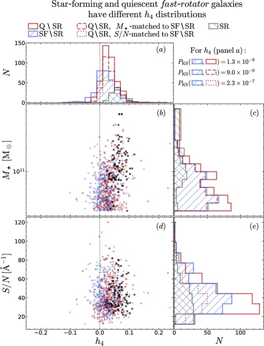
Same as Fig. 7, panels a–e, but removing slow-rotator (SR) galaxies. The latter are represented by the black squares and black hatched histogram. SRs have larger average h4 than fast-rotator galaxies (panel a, cf. empty red and hatched blue histograms versus hatched black histogram). However, removing SRs reduces – but does not remove – the difference in h4 between star-forming and quiescent galaxies. This is true even after matching quiescent galaxies in M⋆ or S/N to the star-forming galaxies.
5.2 Correlations with galaxy projected shape and rotation-to-dispersion ratio
Guided by our toy models (Section 2), we now study how h4 is related to projected axis ratio q and to the ratio between rotation and dispersion (V/σ)e, which are two other tracers of orbital structure7 (e.g. Binney 1978; Davies et al. 1983; Cappellari et al. 2007; Emsellem et al. 2011). In Fig. 9, we show the q–(V/σ)e plane, where the symbols represent individual galaxies, colour-coded by h4. The left/right columns show star-forming/quiescent galaxies (represented as circles/diamonds), and the three rows from top to bottom correspond to SAMI, MAGPI, and LEGA-C data. In each panel, the black arrows are a graphical representation of the PCCs (the grey arrows are the 16th and 84th percentiles of the distribution of angles after bootstrapping each subset 1000 times). The value of the PCCs, the associated p values, and the resulting angle θ are reported in Table 3; rows 1–12, columns 7–9. We highlight in bold correlations that are statistically significant, assumed here to have p < 10−3 (we recall that (V/σ)e has two different meanings: for SAMI and MAGPI, it is the observed ratio within one Re, whereas for LEGA-C it is a model-inferred ratio evaluated at one Re; Section 3.3.3).
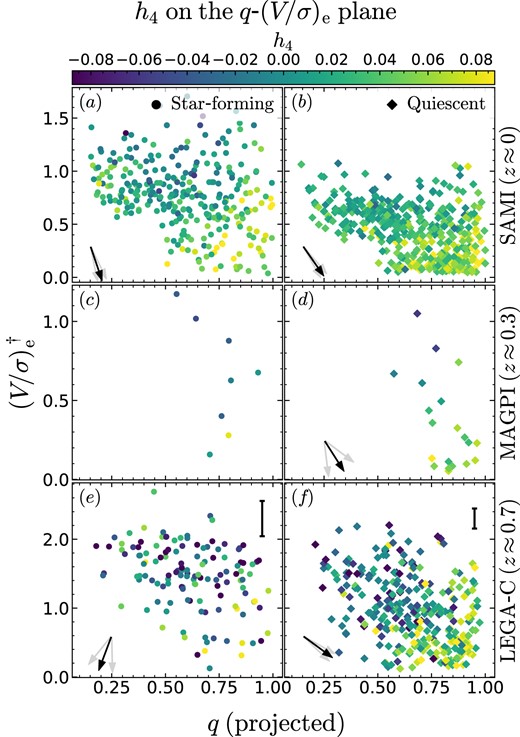
Our samples on the shape–rotation-to-dispersion plane, colour-coded by h4. The left/right columns show star-forming/quiescent galaxies, the top/middle/bottom rows show the SAMI/MAGPI/LEGA-C sample. The direction of the black arrows indicates the relative strength of the h4 –q and h4 –(V/σ)e correlations (grey arrows show the 16th–84th range from bootstrapping). The numerical value of the PCCs and the angle of the arrows are reported in Table 3, rows 1–12. The strong relation between h4, (V/σ)e and projected q highlights that these three parameters capture different aspects of the orbital structure of a galaxy. † (V/σ)e has two different meanings for SAMI and MAGPI versus LEGA-C: for SAMI and MAGPI, it is the observed value inside one Re, for LEGA-C it is the best-fitting model value at one Re (Section 3.3.3). However, our aim is to show how h4 relates to the degree of rotation support, not to quantify this dependence as a function of redshift.
Partial correlations of h4 with (V/σ)e and q (rows 1–12), M⋆ and Re (rows 13–24), M⋆ and σap (rows 25–36), and M⋆ and (V/σ)e (rows 37–48). Statistically significant correlations (p < 10−3) are highlighted in bold. The strongest and most significant correlations are with (V/σ)e, followed by M⋆. For MAGPI, the lack of correlation is likely due to the small sample size. For SAMI, the reported trends persist if we exclude SR galaxies (but the p values are lower).
| Survey | Subset | N | PCC | ρ | P | θ | ||
|---|---|---|---|---|---|---|---|---|
| (1) | (2) | (3) | (4) | (5) | (6) | (7) | (8) | (9) |
| q-(V/σ)e plane | (1) | SAMI | SF | 298 | ρ(h4, q|(V/σ)e) | 0.17(0.11, 0.26) | 4.0 × 10⁻³ | −69.9(− 77.2, −62.8) |
| (2) | |$\boldsymbol {\rho (h_4, (V/\sigma)_\mathrm{e} \vert q)}$| | −0.45(− 0.47, −0.51) | |$\mathbf {1.5 \times 10^{-16}}$| | |||||
| (3) | Q | 423 | |$\boldsymbol {\rho (h_4, q \vert (V/\sigma)_\mathrm{e})}$| | 0.32(0.26, 0.39) | |$\mathbf {3.0 \times 10^{-11}}$| | −53.0(− 58.5, −47.2) | ||
| (4) | |$\boldsymbol {\rho (h_4, (V/\sigma)_\mathrm{e} \vert q)}$| | −0.42(− 0.42, −0.42) | |$\mathbf {1.7 \times 10^{-19}}$| | |||||
| (5) | MAGPI | SF | 8 | ρ(h4, q|(V/σ)e) | 0.51(0.17, 0.59) | 2.5 × 10⁻¹ | −59.6(− 79.4, −45.0) | |
| (6) | ρ(h4, (V/σ)e|q) | −0.86(− 0.93, −0.59) | 1.2 × 10⁻² | |||||
| (7) | Q | 20 | ρ(h4, q|(V/σ)e) | 0.38(0.05, 0.65) | 1.1 × 10⁻¹ | −55.4(− 84.8, −34.3) | ||
| (8) | ρ(h4, (V/σ)e|q) | −0.55(− 0.58, −0.45) | 1.6 × 10⁻² | |||||
| (9) | LEGA-C | SF | 132 | ρ(h4, q|(V/σ)e) | −0.09(− 0.16, 0.01) | 3.1 × 10⁻¹ | −112.0(− 131.0, −87.6) | |
| (10) | ρ(h4, (V/σ)e|q) | −0.22(− 0.18, −0.18) | 1.2 × 10⁻² | |||||
| (11) | Q | 297 | |$\boldsymbol {\rho (h_4, q \vert (V/\sigma)_\mathrm{e})}$| | 0.40(0.33, 0.47) | |$\mathbf {1.7 \times 10^{-12}}$| | −34.2(− 42.3, −27.0) | ||
| (12) | |$\boldsymbol {\rho (h_4, (V/\sigma)_\mathrm{e} \vert q)}$| | −0.27(− 0.30, −0.24) | |$\mathbf {2.7 \times 10^{-6}}$| | |||||
| M⋆ -Re plane | (13) | SAMI | SF | 314 | |$\boldsymbol {\rho (h_4, M_\star \vert R_\mathrm{e})}$| | 0.19(0.24, 0.19) | |$\mathbf {5.4 \times 10^{-4}}$| | −13.0(− 27.6, 4.5) |
| (14) | ρ(h4, Re|M⋆) | −0.04(− 0.12, 0.01) | 4.3 × 10⁻¹ | |||||
| (15) | Q | 451 | |$\boldsymbol {\rho (h_4, M_\star \vert R_\mathrm{e})}$| | 0.24(0.25, 0.19) | |$\mathbf {2.8 \times 10^{-7}}$| | 17.5(5.2, 31.3) | ||
| (16) | ρ(h4, Re|M⋆) | 0.08(0.02, 0.12) | 1.1 × 10⁻¹ | |||||
| (17) | MAGPI | SF | 8 | ρ(h4, M⋆|Re) | 0.26(0.13, −0.37) | 5.8 × 10⁻¹ | −42.5(− 73.7, 116.3) | |
| (18) | ρ(h4, Re|M⋆) | −0.24(− 0.44, 0.75) | 6.1 × 10⁻¹ | |||||
| (19) | Q | 21 | ρ(h4, M⋆|Re) | 0.20(0.19, −0.00) | 3.9 × 10⁻¹ | 34.3(− 22.2, 90.5) | ||
| (20) | ρ(h4, Re|M⋆) | 0.14(− 0.08, 0.33) | 5.6 × 10⁻¹ | |||||
| (21) | LEGA-C | SF | 326 | ρ(h4, M⋆|Re) | 0.18(0.17, 0.18) | 1.3 × 10⁻³ | −33.3(− 41.9, −22.0) | |
| (22) | ρ(h4, Re|M⋆) | −0.12(− 0.15, −0.07) | 3.6 × 10⁻² | |||||
| (23) | Q | 764 | |$\boldsymbol {\rho (h_4, M_\star \vert R_\mathrm{e})}$| | 0.14(0.19, 0.13) | |$\mathbf {9.5 \times 10^{-5}}$| | 41.3(26.1, 55.4) | ||
| (24) | |$\boldsymbol {\rho (h_4, R_\mathrm{e} \vert M_\star)}$| | 0.12(0.09, 0.19) | |$\mathbf {6.1 \times 10^{-4}}$| | |||||
| M⋆ -σap plane | (25) | SAMI | SF | 242 | ρ(h4, M⋆|σap) | 0.21(0.15, 0.15) | 1.3 × 10⁻³ | −30.4(− 40.8, −17.7) |
| (26) | ρ(h4, σap|M⋆) | −0.12(− 0.13, −0.05) | 6.1 × 10⁻² | |||||
| (27) | Q | 409 | |$\boldsymbol {\rho (h_4, M_\star \vert \sigma _\mathrm{ap})}$| | 0.29(0.35, 0.25) | |$\mathbf {3.2 \times 10^{-9}}$| | −14.4(− 21.7, −5.7) | ||
| (28) | ρ(h4, σap|M⋆) | −0.07(− 0.14, −0.03) | 1.4 × 10⁻¹ | |||||
| (29) | MAGPI | SF | 8 | ρ(h4, M⋆|σap) | 0.11(− 0.81, 0.89) | 8.1 × 10⁻¹ | −15.7(− 134.2, 47.4) | |
| (30) | ρ(h4, σap|M⋆) | −0.03(− 0.83, 0.97) | 9.5 × 10⁻¹ | |||||
| (31) | Q | 22 | ρ(h4, M⋆|σap) | 0.30(0.51, 0.03) | 1.8 × 10⁻¹ | −13.0(− 37.7, 83.2) | ||
| (32) | ρ(h4, σap|M⋆) | −0.07(− 0.39, 0.27) | 7.6 × 10⁻¹ | |||||
| (33) | LEGA-C | SF | 339 | ρ(h4, M⋆|σap) | 0.14(0.21, 0.14) | 8.7 × 10⁻³ | −8.8(− 25.7, 17.4) | |
| (34) | ρ(h4, σap|M⋆) | −0.02(− 0.10, 0.04) | 6.9 × 10⁻¹ | |||||
| (35) | Q | 818 | |$\boldsymbol {\rho (h_4, M_\star \vert \sigma _\mathrm{ap})}$| | 0.37(0.36, 0.35) | |$\mathbf {3.0 \times 10^{-27}}$| | −27.0(− 30.7, −23.2) | ||
| (36) | |$\boldsymbol {\rho (h_4, \sigma _\mathrm{ap} \vert M_\star)}$| | −0.19(− 0.21, −0.15) | |$\mathbf {7.6 \times 10^{-8}}$| | |||||
| M⋆ -(V/σ)e plane | (37) | SAMI | SF | 298 | ρ(h4, M⋆|(V/σ)e) | 0.04(− 0.02, 0.12) | 4.6 × 10⁻¹ | −85.0(− 92.1, −77.4) |
| (38) | |$\boldsymbol {\rho (h_4, (V/\sigma)_\mathrm{e} \vert M_\star)}$| | −0.49(− 0.55, −0.53) | |$\mathbf {2.6 \times 10^{-19}}$| | |||||
| (39) | Q | 423 | |$\boldsymbol {\rho (h_4, M_\star \vert (V/\sigma)_\mathrm{e})}$| | 0.19(0.16, 0.25) | |$\mathbf {5.9 \times 10^{-5}}$| | −67.5(− 73.4, −61.1) | ||
| (40) | |$\boldsymbol {\rho (h_4, (V/\sigma)_\mathrm{e} \vert M_\star)}$| | −0.47(− 0.53, −0.45) | |$\mathbf {2.2 \times 10^{-24}}$| | |||||
| (41) | MAGPI | SF | 8 | ρ(h4, M⋆|(V/σ)e) | 0.36(− 0.33, 0.82) | 4.3 × 10⁻¹ | −67.8(− 112.6, −47.0) | |
| (42) | ρ(h4, (V/σ)e|M⋆) | −0.87(− 0.80, −0.88) | 1.0 × 10⁻² | |||||
| (43) | Q | 20 | ρ(h4, M⋆|(V/σ)e) | 0.21(− 0.04, 0.37) | 3.9 × 10⁻¹ | −70.2(− 94.2, −49.4) | ||
| (44) | ρ(h4, (V/σ)e|M⋆) | −0.59(− 0.55, −0.43) | 8.3 × 10⁻³ | |||||
| (45) | LEGA-C | SF | 132 | ρ(h4, M⋆|(V/σ)e) | 0.15(0.08, 0.24) | 7.7 × 10⁻² | −51.7(− 72.1, −31.1) | |
| (46) | ρ(h4, (V/σ)e|M⋆) | −0.20(− 0.26, −0.15) | 2.5 × 10⁻² | |||||
| (47) | Q | 297 | |$\boldsymbol {\rho (h_4, M_\star \vert (V/\sigma)_\mathrm{e})}$| | 0.25(0.23, 0.28) | |$\mathbf {1.4 \times 10^{-5}}$| | −54.8(− 63.0, −47.1) | ||
| (48) | |$\boldsymbol {\rho (h_4, (V/\sigma)_\mathrm{e} \vert M_\star)}$| | −0.35(− 0.45, −0.31) | |$\mathbf {3.4 \times 10^{-10}}$| |
Note. Columns: (1) reference to the relevant figure; (2) unique row identifier; (3) data source; (4) Q/SF for the quiescent/star-forming subsets; (5) number of galaxies in the current subset, after removing galaxies that do not possess the necessary measurements to calculate the PCC; (6) PCC in this row; (7) value of the PCC, with the numbers in parentheses encompassing the 16th–84th percentiles from 1000 bootstrapping realizations; (8) p value associated with the PCC (probability that a PCC as large as reported arised from uncorrelated data); (9) angle representation of the complementary PCCs, with the number in parentheses encompassing the 16th–84th percentiles from bootstrapping (see Section 5 and Bluck et al. 2020a for a definition).
For SAMI and LEGA-C, we have large enough samples to observe the well-known anticorrelation between (V/σ)e and q (see e.g. Emsellem et al. 2011, their fig. 6, where ϵe ∼ 1 − q). If we look at the correlation coefficient between h4 and either of these two parameters, we find in both cases a statistically significant correlation.
To disentangle the (V/σ)e –q anticorrelation from the relation with h4, in the following text we always use PCCs. The PCCs between q and h4 while controlling for (V/σ)e are reported in rows 1, 3, 5, 7, 9, and 11 of Table 3; the PCCs between (V/σ)e and h4 while controlling for q are reported in rows 2, 4, 6, 8, 10, and 12. In general, h4 anticorrelates with (V/σ)e: this is true for SAMI (rows 2 and 4 in Table 3) and for LEGA-C quiescent galaxies (row 12). For MAGPI, none of the PCCs are significant, likely due to the small sample size, but we highlight that the anticorrelation between h4 and (V/σ)e has particularly low P (row 8, column 8); this possible anticorrelation can also be appreciated in the clear gradient of colour hues in panel c. Finally, for LEGA-C and MAGPI star-forming galaxies, we find no correlation with (V/σ)e.
Unlike for (V/σ)e, the relation between h4 and q is related to the star-forming status of galaxies. For star-forming galaxies, the h4–q correlation is weak (SAMI) or not significant (MAGPI and LEGA-C). This is expected from the fact that the star-forming subsets are dominated by intrinsically flat systems, for which projected shape q is driven primarily by the random viewing angle. In contrast, for quiescent galaxies, we find a positive correlation for both SAMI and LEGA-C (rows 3 and 11). The PCCs are larger than the values found for star-forming galaxies (column 7, cf. rows 1 and 3, and 9 and 11). Because projected shape q is also related to intrinsic shape, this correlation suggests that intrinsically round galaxies tend to have higher h4.
We remark that, for SAMI, the h4–(V/σ)e correlation has larger PCC and higher statistical significance than the h4–q correlation, but the opposite is true for LEGA-C quiescent galaxies. However, because (V/σ)e is calculated differently between the two samples (Section 3.3.3), we cannot say if the different importance of the two correlations is meaningful.
In summary, we find statistically significant correlations of h4 with (V/σ)e and q in three out of six subsets (three out of four subsets excluding MAGPI, which has <25 galaxies). This confirms that our spatially integrated h4 contains kinematic information related to the orbital structure of stars in galaxies, an independent validation of our measurements. Because we use PCCs, the strong anticorrelation between (V/σ)e and q is always removed when calculating the correlations with h4. For this reason, the separate existence of the h4–q and h4–(V/σ)e correlations means that, for quiescent galaxies, h4 contains independent orbital information that is captured separately by q and (V/σ)e. We note that none of the above conclusions change if we change the quality selection criteria from |$u(h_4\,) \lt 0.05$| to a stricter cut |$u(h_4\,) \lt 0.03$|.
5.3 Correlations with galaxy mass and size
The relation of h4 with stellar mass and size is illustrated in Fig. 10. In all panels except c, we observe a correlation between M⋆ and Re (Shen et al. 2003). We remark that the mass distribution of the three samples is not the same, with LEGA-C probing on average more massive galaxies than SAMI, for both the quiescent and star-forming subsets (cf. Fig. 6). Despite this different selection, we can appreciate by eye the increase in average Re between the look-back times of LEGA-C and SAMI (van der Wel et al. 2014). The PCCs and angle are reported in Table 3; rows 13–24, columns 7–9.
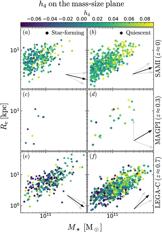
Our galaxies on the mass–size plane, colour-coded by h4. The symbols are the same as Fig. 9. The numerical value of the PCCs and the angle of the arrows are reported in Table 3, rows 2–24. All the arrows fall in the first or fourth quadrant, consistent with a positive h4–M⋆ correlation after controlling for Re. For LEGA-C quiescent galaxies, we also find evidence for a correlation between h4 and Re, after controlling for M⋆. The negative h4–Re correlation for LEGA-C star-forming galaxies (panel e) is not statistically significant.
For star-forming galaxies (panels a, c, and e), the black arrows lie in the fourth quadrant, suggesting that h4 correlates with M⋆ but anticorrelates with Re. However, quantitatively, the only statistically significant correlation is the h4–M⋆ correlation for SAMI star-forming galaxies; the sample size for MAGPI is probably too small, whereas for LEGA-C, the p value corresponds to three standard deviations, very close but above the adopted significance threshold (p < 10−3). In contrast, we find no statistical evidence for the h4–Re anticorrelation.
For quiescent galaxies (panels b, d, and f), the black arrows lie in the first quadrant, indicating that h4 correlates with both M⋆ and Re. However, quantitatively, only the LEGA-C sample shows statistically significant independent correlations of h4 with M⋆ and Re. For MAGPI, there is no evidence of a correlation with M⋆ either.
5.4 Correlations with stellar mass and aperture velocity dispersion
Alongside M⋆, a key galaxy observable is the second moment of the aperture-integrated LOSVD, σap (Section 3.3.3). This kinematic observable is of particular interest because, compared to M⋆, relative changes in σap are small during the evolution of a galaxy (e.g. Bezanson et al. 2009; Naab, Johansson & Ostriker 2009; Oser et al. 2012; van de Sande et al. 2013 – with the exception of the initial phases of rapid gas accretion and star formation). Our findings are illustrated in Fig. 11 and reported in Table 3; rows 25–36.
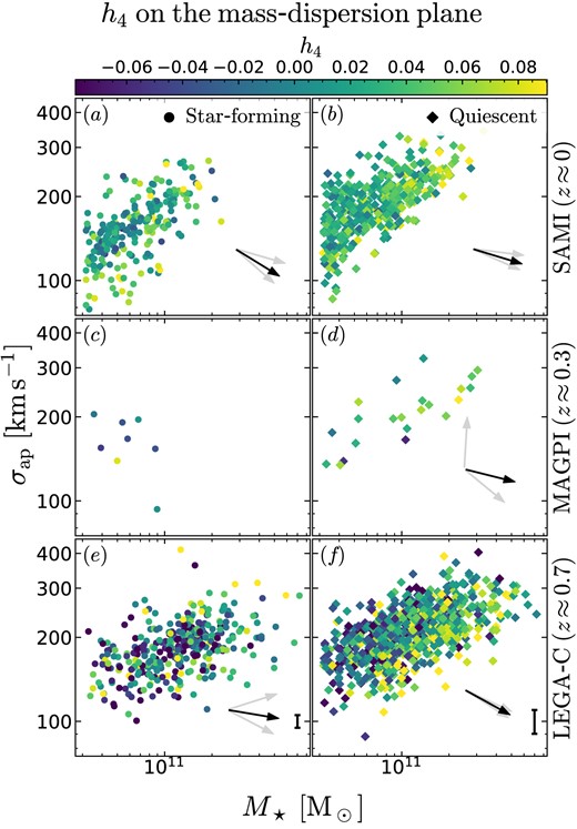
Our galaxies on the mass–dispersion plane, colour-coded by h4. The symbols are the same as Fig. 9, the PCCs and the angle of the arrows are reported in Table 3, rows 25–36. h4 correlates more strongly with M⋆ than with aperture velocity dispersion σap, both for local quiescent galaxies (panel c) and for quiescent galaxies at z = 0.7 (panel f). After the dissipative formation phase, changes in σap are only fractional, while M⋆ may more than double via gas-poor mergers. Therefore, positive correlations of h4 with M⋆ (after controlling for σap) are suggestive of non-dissipative mass growth.
The direction of the arrows indicates clearly that, between M⋆ and σap, it is M⋆ that correlates most strongly with h4. However, statistically, we find significant h4–M⋆ correlations only for SAMI and LEGA-C quiescent galaxies. For LEGA-C quiescent galaxies, we find a statistically significant anticorrelation with σap; interestingly, this negative correlation disappears if we replace σap with its inclination-corrected equivalent σvir (van der Wel et al. 2022).
5.5 Correlations with galaxy mass and rotation-to-dispersion ratio
Having determined that M⋆ and (V/σ)e are the best predictors of h4, we now compare these two observables directly. The M⋆–(V/σ)e plane is shown in Fig. 12, with the usual meaning of the symbols; the relevant PCCs are reported in Table 3, rows 37–48.
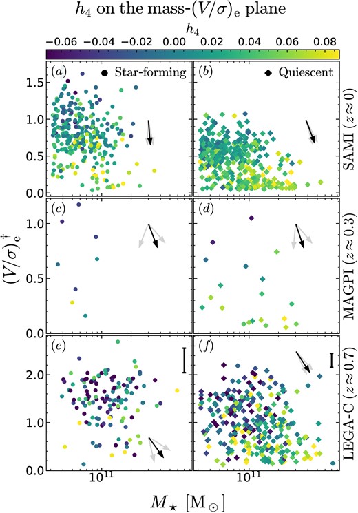
Our galaxies on the M⋆–(V/σ)e plane, colour-coded by h4. The left/right columns show star-forming/quiescent galaxies, and the top/middle/bottom rows show the SAMI/MAGPI/LEGA-C samples. The symbols are the same as Fig. 10, the PCCs and the angle of the arrows are reported in Table 3, rows 37–48. In general, the h4–(V/σ)e correlations are stronger than the h4–M⋆ correlations; the latter only exist independently for LEGA-C quiescent galaxies, and, perhaps, for SAMI quiescent galaxies. † (V/σ)e has two different meanings for SAMI and MAGPI versus LEGA-C. See also note to Fig. 9 and Section 3.3.3.
For SAMI star-forming galaxies, after controlling for (V/σ)e, there is no evidence of the h4–M⋆ correlation (cf. rows 37 and 38). In contrast, for quiescent galaxies, we find evidence of an independent h4–M⋆ correlation for both SAMI (row 39) and LEGA-C (row 47). In all three cases, the h4–(V/σ)e correlations have larger magnitude and higher statistical significance than the h4–M⋆ correlations (rows 38, 40, and 48). In summary, h4 reflects much more (V/σ)e than M⋆, but the correlation with M⋆ is independent of the h4–(V/σ)e correlation, highlighting again that integrated h4 is more than just (V/σ)e.
6 DISCUSSION
6.1 Relation between h4 and rotation
Overall, the almost ubiquitous h4–(V/σ)e anticorrelation (Fig. 9) means that our integrated, light-weighted h4 probes mostly (light-weighted) rotation-to-dispersion ratio. This strong anticorrelation is found not only in the data, but is also predicted by our (admittedly simple) kinematic models (cf. Figs 1 and 9). Indeed, the h4–(V/σ)e anticorrelation is strong enough that we have tentative evidence even for only 20 galaxies in the MAGPI quiescent sample. In this light, the different h4 between star-forming and quiescent galaxies (Fig. 7) reflects to a large degree the known difference in (V/σ)e between these two populations (e.g. Graham et al. 2018; van de Sande et al. 2018; Falcón-Barroso et al. 2019).
When we consider projected shape, we find that for star-forming galaxies, the h4–q correlation is either not detected (for MAGPI and LEGA-C) or, when detected, the correlation coefficient has smaller magnitude and lower statistical significance than the h4–(V/σ)e anticorrelation (Table 3, rows 1–2). These results are in agreement with our toy models, as expected from the fact that in the mass range explored here, star-forming galaxies have predominantly disc-like kinematics.
In contrast, for quiescent galaxies, h4 has strong independent correlations with both (V/σ)e and projected q – as expected from the fact that these two observables capture independent aspects of galaxy kinematics (Illingworth 1977; Binney 1978; Davies et al. 1983). The measured h4–q correlation (Table 3, rows 3–4 and 11–12) has larger correlation coefficient than predicted by our thin-disc models (Table 1). This is not surprising (quiescent galaxies are not thin-discs) but also suggests that h4 measures more than just (V/σ)e – at least for quiescent galaxies. In fact, for bulge-like structures, q reflects (statistically) the intrinsic axis ratio, which in turn is related to kinematic properties such as orbital anisotropy; so, for quiescent galaxies, the h4–q correlation compounds inclination effects with physical trends. This combination may explain why we find the h4–q correlation in quiescent galaxies to have larger magnitude and higher statistical significance compared to the same relation for star-forming galaxies, even after taking into account the different sample sizes.
For SAMI quiescent galaxies, h4 correlates more strongly with (V/σ)e than with q, but for LEGA-C the opposite is true; this fact could be due to the different spatial resolution between the two surveys (for SAMI, (V/σ)e is measured on kpc scales, whereas LEGA-C spatial resolution is approximately 7 kpc), or to a genuine change in the population demographics over the last 7 Gyr. However, we recall that (V/σ)e is defined and measured differently between the two data sets (Section 3.3.3), so a direct comparison is unwarranted and we defer it to future work.
6.2 Fast- and slow-rotator quiescent galaxies
The reported trends of h4 with (V/σ)e and q persist for the sample of FR quiescent galaxies. Moreover, we have shown explicitly that star-forming galaxies and fast-rotator quiescent galaxies have different h4 distributions, but that the difference becomes larger if we include SR quiescent galaxies (Section 5.1.2). These facts show that fast-rotator quiescent galaxies are intermediate between star-forming and SR systems. The existence of a separate population of SR (i.e. a bimodality in the kinematics of quiescent galaxies, Emsellem et al. 2007; Cappellari 2016; Graham et al. 2018; van de Sande et al. 2021a) is relevant to understanding how stellar orbits transform from rotation supported (as imprinted from the kinematics of star-forming gas) to dispersion supported (as observed in SRs). From the point of view of h4, we see evidence of a gradual transformation between star-forming galaxies and fast-rotator quiescent galaxies, which shows that there is some degree of gradual transformation. We see no evidence for a bimodality in the h4 distribution of quiescent galaxies, but our number statistics are probably too low to detect it (see van de Sande et al. 2021a).
6.3 Relation between h4 and dry mergers
When we study h4 in relation to M⋆ and (V/σ)e, we find that, once again, h4 is driven primarily by (V/σ)e (Fig. 12 and Table 3, rows 37–48). However, for quiescent galaxies, the h4 –M⋆ correlation exists independently of (V/σ)e. This fact confirms that integrated h4 is not just (V/σ)e, and that some of the variability in h4 at fixed (V/σ)e might be physically associated with processes that increase M⋆. For LEGA-C quiescent galaxies, we also find evidence for an independent correlation between h4 and Re, such that, at fixed M⋆, the largest galaxies also have the highest h4. Given the strength of this correlation, if it was present in SAMI data we should be able to detect it, even after accounting for the different sample size. Aperture effects do not explain the difference: measuring the SAMI h4 inside a slit does not change our results (cf. the mock-slit spectra from D’Eugenio et al. 2023). A possible explanation is that SAMI quiescent galaxies are on average less massive than LEGA-C quiescent galaxies. Indeed, if we resample the latter to match the M⋆ distribution of the SAMI quiescent sample, the h4–Re correlation disappears. However, the resulting M⋆-matched sample is relatively small, so this test is not conclusive.
Of particular interest is the lack of correlation with σap (Fig. 11 and Table 3, rows 25–36). We find only correlations with M⋆ (for SAMI and LEGA-C quiescent galaxies) or marginal evidence of correlations with M⋆ (for SAMI and LEGA-C star-forming galaxies and for MAGPI quiescent galaxies). For LEGA-C, we even find a negative correlation between h4 and σap (p = 7.6 × 10⁻⁸), but this may be due to inclination effects.8
Taken together, these results suggest that h4 may be related to gas-poor (dry) mergers: these decrease (V/σ)e, increase both M⋆ and Re and leave σap unchanged (for major mergers) or lower it very little (for minor mergers, Bezanson et al. 2009; Naab et al. 2009; Oser et al. 2012; van de Sande et al. 2013). In principle, h4 may reflect dynamical heating due to secular processes, which could also induce an anticorrelation between resolved h4 and (V/σ)e. However, if we assume dynamical heating to go together with stellar-population age, we would then expect an independent correlation between h4 and σap at fixed M⋆ (because σap predicts age more accurately than M⋆, McDermid et al. 2015; Scott et al. 2017; Barone et al. 2018, 2020), which is ruled out by our data (Fig. 11).
6.4 Relation between integrated and spatially resolved h4
In addition to the h4–(V/σ)e anticorrelation, our toy models also predict an equally strong correlation between integrated and spatially resolved h4 (Fig. 2). To probe this correlation, we used two cuts (in q and (V/σ)e) designed to suppress the h4–(V/σ)e anticorrelation and to enhance the correlation between integrated and resolved h4 (Table 1). Comparing integrated h4 between star-forming and quiescent galaxies for q ≥ 0.75, we still find a statistically significant difference, but no difference is found for |$(V/\sigma)_\mathrm{e}\, \le 0.5$| (Section 5.1). Given that – with these selections – there is a strong correlation between integrated and resolved h4, the lack of difference means that either star-forming and quiescent galaxies have the same value of resolved h4 (i.e. any difference in integrated h4 is driven entirely by (V/σ)e), or, alternatively, that resolved h4 varies jointly with (V/σ)e.
Theoretically, resolved h4 measures radial anisotropy (Gerhard 1993; van der Marel & Franx 1993), so a link between resolved h4 and (V/σ)e seems natural: thin discs are by definition low-dispersion systems generated by dissipative cold-gas accretion, while radial anisotropy is associated with dissipationless accretion.
6.5 Insight from spatially resolved spectroscopy
Spatially resolved h4 measurements from integral-field spectroscopy show complex structure (Emsellem et al. 2004), which complicates the interpretation of our spatially integrated measurements. In fact, our h4 could be due not only to radial anisotropy versus rotation, but also to bars (e.g. peanut-shaped bulges, Debattista et al. 2005; Méndez-Abreu et al. 2008) and kinematically decoupled cores (see e.g. Emsellem et al. 2004, their fig. 4). Indeed, after employing the visual bar classification performed by the SAMI team on HSC (Aihara et al. 2019), Pan-STARRS (Chambers et al. 2016; Flewelling et al. 2020), and Decals (Dey et al. 2019) imaging, we find a weak anticorrelation between integrated h4 and the probability that a bar is present. However, after controlling for M⋆ or (V/σ)e, this correlation disappears, so it is unlikely that bars are responsible for the trends we observe. A larger sample, perhaps with better spatial resolution, may help clarify whether an independent correlation with integrated h4 is present.
Following Krajnović et al. (2011), van de Sande et al. (2017b) divided the SAMI galaxies between regular and non-regular rotators, and found that both classes display the full range of h4 values (cf. their fig. 9). However, regular rotators also show a strong radial h4 gradient, with their central regions having |$h_4\, \lesssim 0$| (van de Sande et al. 2017b, fig. 9, panels d and f). Because these central low-h4 regions are brighter than the high-h4 outskirts, it is reasonable to assume that our integrated h4 measurements are lower for regular rotators than for non-regular rotators, where the central regions display |$h_4\, \approx 0.05$| (van de Sande et al. 2017b).
The fact that on average our star-forming galaxies have lower h4 than quiescent galaxies is qualitatively consistent with the expectation that, in the stellar-mass range explored here, star-forming galaxies are overwhelmingly regular rotators (or ‘dynamically cold discs’ Fraser-McKelvie & Cortese 2022). On the other hand, even though massive non-regular rotators are predominantly quiescent, the converse is not true: quiescent galaxies are also dominated by regular rotators, which account for 60–80 per cent of the local early-type galaxy population (see e.g. Cappellari et al. 2011; van de Sande et al. 2017a). The degree to which the fraction of quiescent galaxies that are non-regular rotators ‘skews’ the h4 distribution to higher values is hard to determine: ideally we would like to control for stellar mass by comparing three M⋆-matched samples: star-forming regular rotators (the control sample), quiescent regular rotators, and quiescent non-regular rotators. However, non-regular rotators have distinctively higher M⋆ (Brough et al. 2017; Veale et al. 2017; van de Sande et al. 2021b), so matching in M⋆ is not feasible. Nevertheless, a KS test between star-forming and quiescent regular rotators gives a p value of 0.03, which is indecisive; larger sample sizes are needed to clarify whether this difference is significant.
We note that, in principle, the shape of the gravitational potential also affects the LOSVD. The fact that star-forming and quiescent galaxies have different light distributions means that they are likely to have different potentials too. However, in practice, orbital distribution (regardless of the origin) is the dominant factor in determining h4, with the detailed shape of the gravitational potential being a second-order effect (Gerhard 1993).
6.6 Difference between star-forming and quiescent galaxies
In Section 5.1, we have studied the relation between h4, M⋆, and S/N using SAMI and LEGA-C data. For both surveys, and for both quiescent and star-forming galaxies, we find a statistically significant correlation between h4 and M⋆. In comparison, the correlation between h4 and S/N is either less statistically significant or not detected. The contrast between the h4–M⋆ correlations and the weaker or absent correlations with S/N gives us confidence that our h4 measurements trace a physical property of the galaxies, not the S/N of the spectra.
At fixed M⋆, the h4 distribution has large intrinsic scatter, suggesting a large degree of physical variability, probably reflecting the broad range in q, (V/σ)e, and integrated h4 of the sample.
The main result of Section 5.1 is that quiescent and star-forming galaxies have different h4 distributions, even after matching their M⋆ or S/N distributions; this is true both in the local Universe (SAMI, Fig. 7a) and 7 Gyr ago9 (LEGA-C, Fig. 7f; note that, for the ongoing MAGPI Survey, the current sample size is too small for this analysis). We also checked that for SAMI the difference persists after matching the star-forming and quiescent subsets in central velocity dispersion, which is related to quenching (e.g. Bluck et al. 2016, 2020a, b). If a connection between h4 and quenching exists, it must be due to resolved h4 (i.e. radial anisotropy) and not (V/σ)e, because the latter has already been ruled out as a driver of galaxy quenching (Brownson et al. 2022). However, the differences in integrated h4 between star-forming and quiescent galaxies are small compared to the differences in central dispersion (Bluck et al. 2016, 2020a). Future work on this subject may clarify the likelihood of a causal connection with quenching.
Moving to the link between h4 and other galaxy observables (Figs 9–12), whenever we find statistically significant trends for both star-forming and quiescent galaxies, their direction agrees. This fact suggests that the same physical mechanisms may be determining h4 in both star-forming and quiescent galaxies, with the differences in median value and statistical significance due to different relative contribution.
6.7 Predicting rotation from integrated h4
The strong h4–(V/σ)e anticorrelation raises the question whether we can use integrated h4 (which can be measured from relatively inexpensive single-fibre observations) to infer (V/σ)e (which requires slit or fibre spectroscopy). The relation between h4 and (V/σ)e for SAMI is shown in Fig. 13(a), where blue circles/red diamonds represent star-forming/quiescent galaxies. We used the least-trimmed squares algorithm to fit a linear relation (Rousseeuw & Driessen 2006; Cappellari et al. 2013). The observed scatter about the linear best-fitting relation is 0.23 (considering star-forming and quiescent galaxies together), or 0.16 for quiescent galaxies alone; this is dominated by intrinsic scatter (0.15 and 0.10, respectively). While the large intrinsic scatter is in agreement with our hypothesis that h4 contains more information than just (V/σ)e, it also means that we cannot use single-fibre observations to accurately measure (V/σ)e. To make matters worse, we obtain similar scatter if we replace h4 with q, which can be measured from imaging alone (Fig. 13b). In this case, the observed scatter is 0.20 (0.14 for quiescent galaxies) and the intrinsic scatter is 0.17 (0.11 for quiescent galaxies). It remains to be seen whether combining h4 with q or with other observables can improve our estimate of (V/σ)e.
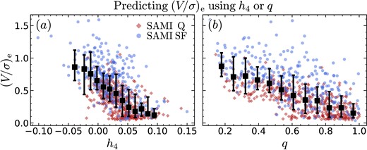
As a predictor of (V/σ)e, h4 (panel a) performs similarly to projected axis ratio q (panel b). The blue circles/red diamonds are SAMI star-forming/quiescent galaxies, the black squares are the running median, with the errorbars encompassing the 16th–84th percentiles of the data. Using h4 alone, one can predict (V/σ)e with a typical uncertainty of 0.23, which reduces to 0.16 if considering only quiescent galaxies; these results are similar to what we would get using galaxy shape q instead of h4.
6.8 Caveats and future outlook
There are two difficulties with our interpretation of h4 being related to dry mergers. First, a key prediction of the dry merger hypothesis is that it affects the outskirts (R > Re) more than the central regions. Even though we observe our galaxies in projection (so part of the outskirts are probed along the line of sight), the magnitude of the expected signal is unclear. A comparison with numerical simulations would be beneficial. Resolved studies have shown that – for regular rotators – the central regions have indeed lower h4, as expected from this scenario (van de Sande et al. 2017b, their fig. 9d). However, the picture for non-regular rotators is not as clear, with the centre possibly having higher h4 (Emsellem et al. 2004, their fig. 4). A quantitative study of the radial distribution of h4 over a large sample of galaxies could address this question. A second prediction of the dry merger hypothesis is that it would lead to mass and even stronger size growth, yet we find almost no evidence of independent correlations between h4 and Re (Fig. 10, Table 3, rows 13–24). The only exception are LEGA-C quiescent galaxies, where the h4–M⋆ and h4–Re correlations have comparable PCCs and significance (rows 23–24). There are two possible explanations why the h4–Re correlation is not observed in the other samples, and especially in the SAMI quiescent sample. The first is that the mass ranges are different, with LEGA-C probing more massive galaxies than SAMI. However, other effects may be hiding the h4–Re correlation. For example, if star-forming galaxies transition to quiescence without significant changes to their size and kinematics, this would add newly quiescent galaxies that are large (because star-forming galaxies are on average larger than quiescent galaxies of the same mass) but have low h4. However, after accounting for M⋆, we find no evidence of an independent correlation between h4 and stellar-population age (we used the light-weighted age measurements from Scott et al. 2017). Future studies based on larger samples may help answer some of the open questions.
Compared to (V/σ)e, h4 presents the advantage of requiring no spatial information, so it can be measured for large single-fibre surveys such as the Sloan Digital Sky Survey (York et al. 2000). As already noted, it may be interesting to explore if and to what extent h4 is related to galaxy quiescence (expanding on the work of Brownson et al. 2022, Piotrowska et al. 2022, and Bluck et al. 2022). Note that the high S/N required to measure h4 may bias the resulting sample, more so than studies based on velocity dispersion alone. With this caveat in mind, the current generation of large single-fibre surveys of the local Universe will give us access to even larger samples than SDSS (e.g. the Dark Energy Spectroscopic Instrument Survey, DESI; DESI Collaboration 2016). Interestingly, the upcoming generation of large single-fibre surveys will include deep spectroscopy that is ideal to measure h4 (e.g. the 4MOST Hemisphere Survey, Taylor et al., in preparation; the WEAVE-StePS Costantin et al. 2019 and 4MOST-StePS surveys; and the DESI Bright Galaxy Survey, Ruiz-Macias et al. 2021), while future high-redshift programs will enable us to study h4 for galaxies at cosmic noon (MOONRISE survey, Maiolino et al. 2020).
7 SUMMARY AND CONCLUSIONS
In this work, we present the first study of integrated h4 for a statistical sample of both star-forming and quiescent galaxies. Using the ppxf software on optical spectroscopy data from the SAMI, MAGPI, and LEGA-C surveys, we model the LOSVD as a Gauss–Hermite series. h4 is the coefficient of the fourth-order Hermite polynomial in the Gauss–Hermite expansion; mathematically, it represents the excess kurtosis. Physically, integrated h4 is related to both the rotation-to-dispersion ratio (V/σ)e and to spatially resolved h4, as we show using a set of simple toy models (Section 2; Figs 1 and 2). We select galaxies with stellar mass |$M_\star \, \gt 10^{10.5} \, \mathrm{M_\odot }\,$|, where, after quality selection (Fig. 5), we are typically 80–98 per cent complete (Fig. 6). For this sample, we find that
The largest magnitude and highest significance correlation is between h4 and (V/σ)e (Sections 5.2 and 5.5, Figs 9 and 12, Table 3, rows 1–12 and 37–48).
After controlling for (V/σ)e, the second-largest magnitude correlation is between h4 and M⋆; this suggests that h4 contains additional information compared to (V/σ)e, in agreement with the models. This information might be connected to mass assembly.
At fixed (V/σ)e or M⋆, the h4 distribution has large intrinsic scatter, reflecting physical variability between galaxies (Sections 5.1 and 6.3).
Quiescent galaxies have larger h4 than coeval star-forming galaxies (Section 5.1, Fig. 7), both in the local Universe (SAMI, z = 0.05) and 7 Gyr ago (LEGA-C, z = 0.7).
When controlling for (V/σ)e, the difference disappears, suggesting that (V/σ)e and resolved h4 vary together.
We interpret h4 as a combination of (V/σ)e and as a measure of the fraction of dry mergers. The latter explains the h4–M⋆ correlation at fixed (V/σ)e, and the lack of independent correlation with σap (Sections 5.4–5.5; Figs 11 and 12).
Given our interpretation, we would expect a correlation between h4 and Re, but this is only detected for LEGA-C quiescent galaxies (Section 5.3). A possible explanation is that the late addition of large, low-h4 star-forming galaxies may hide the h4–Re correlation.
Our results are qualitatively unchanged if we remove slow-rotator galaxies, but the significance of the trends is reduced. Fast-rotator quiescent galaxies have intermediate h4 between star-forming galaxies and slow rotators (Section 5.1.2, Fig. 8c).
ACKNOWLEDGEMENTS
We thank the anonymous referee for insightful comments that greatly improved this article. FDE and AvdW acknowledge funding through the H2020 ERC Consolidator Grant 683184. FDE and RM ackwoledge funding through the ERC Advanced grant 695671 ‘QUENCH’ and support by the Science and Technology Facilities Council (STFC). JvdS acknowledges support of an Australian Research Council Discovery Early Career Research Award (project number DE200100461) funded by the Australian Government. SB acknowledges funding support from the Australian Research Council through a Future Fellowship (FT140101166) ORCID 0000-0002-9796-1363. JJB acknowledges support of an Australian Research Council Future Fellowship (FT180100231). CF is the recipient of an Australian Research Council Future Fellowship (project number FT210100168) funded by the Australian Government. HÜ gratefully acknowledges support by the Isaac Newton Trust and by the Kavli Foundation through a Newton-Kavli Junior Fellowship. LMV acknowledges support by the COMPLEX project from the European Research Council (ERC) under the European Union’s Horizon 2020 research and innovation program grant agreement ERC-2019-AdG 882679.
The SAMI Galaxy Survey is based on observations made at the Anglo-Australian Telescope. The Sydney-AAO Multi-object Integral-field spectrograph (SAMI) was developed jointly by the University of Sydney and the Australian Astronomical Observatory, and funded by ARC grants FF0776384 (Bland-Hawthorn) and LE130100198. The SAMI input catalogue is based on data taken from the Sloan Digital Sky Survey, the GAMA Survey, and the VST ATLAS Survey. The SAMI Galaxy Survey is funded by the Australian Research Council Centre of Excellence for All-sky Astrophysics (CAASTRO), through project number CE110001020, and other participating institutions. The SAMI Galaxy Survey website is http://sami-survey.org/.
Funding for SDSS-III has been provided by the Alfred P. Sloan Foundation, the Participating Institutions, the National Science Foundation, and the U.S. Department of Energy Office of Science. The SDSS-III web site is http://www.sdss3.org/.
GAMA is a joint European-Australasian project based around a spectroscopic campaign using the Anglo-Australian Telescope. The GAMA input catalogue is based on data taken from the Sloan Digital Sky Survey and the UKIRT Infrared Deep Sky Survey. Complementary imaging of the GAMA regions is being obtained by a number of independent survey programmes including GALEX MIS, VST KiDS, VISTA VIKING, WISE, Herschel-ATLAS, GMRT, and ASKAP providing UV to radio coverage. GAMA is funded by the STFC (UK), the ARC (Australia), the AAO, and the participating institutions. The GAMA website is http://www.gama-survey.org/.
Based on observations made with ESO Telescopes at the La Silla Paranal Observatory under programme IDs 179.A-2004. Based on observations collected at the European Organisation for Astronomical Research in the Southern hemisphere under ESO programme 1104.B-0536. We wish to thank the ESO staff, and in particular the staff at Paranal Observatory, for carrying out the MAGPI observations. Part of this research was conducted by the Australian Research Council Centre of Excellence for All Sky Astrophysics in 3 Dimensions (ASTRO 3D), through project number CE170100013.
The Pan-STARRS1 Surveys (PS1) and the PS1 public science archive have been made possible through contributions by the Institute for Astronomy, the University of Hawaii, the Pan-STARRS Project Office, the Max-Planck Society and its participating institutes, the Max Planck Institute for Astronomy, Heidelberg and the Max Planck Institute for Extraterrestrial Physics, Garching, The Johns Hopkins University, Durham University, the University of Edinburgh, the Queen’s University Belfast, the Harvard-Smithsonian Center for Astrophysics, the Las Cumbres Observatory Global Telescope Network Incorporated, the National Central University of Taiwan, the Space Telescope Science Institute, the National Aeronautics and Space Administration under Grant No. NNX08AR22G issued through the Planetary Science Division of the NASA Science Mission Directorate, the National Science Foundation Grant No. AST-1238877, the University of Maryland, Eotvos Lorand University (ELTE), the Los Alamos National Laboratory, and the Gordon and Betty Moore Foundation.
This work extensivey used the freely available Debian GNU/Linux operative system. We used the Python programming language (van Rossum 1995), maintained and distributed by the Python Software Foundation. We further acknowledge direct use of astropy (Astropy Collaboration 2013), ltsfit (Cappellari et al. 2013), matplotlib (Hunter 2007), numpy (Harris et al. 2020), pathos (McKerns et al. 2011), pingouin (Vallat 2018), ppxf (Cappellari 2017), scipy (Jones et al. 2001), and topcat (Taylor 2005).
DATA AVAILABILITY
The reduced data used in this work are available in the public domain. For SAMI, through the SAMI Data Release 3 (Croom et al. 2021a). Ancillary data come from the GAMA Data Release 3 (Baldry et al. 2018) and raw data are from SDSS DR7 (Abazajian et al. 2009), SDSS DR9 (Ahn et al. 2012), and VST (Shanks et al. 2013, 2015). For MAGPI, the raw data (and a basic data reduction) are available through the the ESO Science Archive Facility. For LEGA-C, the raw data and a catalogue of basic photometric and kinematic measurements are available through the ESO Science Archive Facility.
Integrated h4 measurements are available contacting the corresponding author.
Footnotes
Below this stellar mass threshold, star-forming galaxies appear to have rotation-to-dispersion ratios that decrease with decreasing stellar mass (Falcón-Barroso et al. 2019).
But note the non-Gaussian analysis of Krajnović et al. (2011).
Using Sèrsic models with index n higher than one adds weight to the central, low-velocity regions; for this reason, the exponential model is the most conservative in the Sèrsic family with n ≥ 1.
This measurement is conceptually similar to the corresponding measurement for the LEGA-C survey, Section 3.3.3.
Even though Balmer absorption goes against this trend (i.e. it is typically strongest for star-forming galaxy spectra), we mask these spectral regions due to strong contamination from gas emission lines (Appendix A).
It is understood that q also depends on inclination, so its value as a probe of orbital structure is only statistical.
As we noted, this negative correlation disappears if we replace the observed σap with σvir, which includes a multiplicative inclination correction based on the observed axis ratio q (van der Wel et al. 2022).
It would be interesting to compare h4 across the three surveys, but this requires careful matching of the different observing set-ups, and is the subject of a future work (D’Eugenio et al. 2023).
Note that, for the quiescent mocks, |$\langle \Delta \, h_4 \rangle$| is not consistent with 0, i.e. we recover a biased value of h4. The reason for this bias is not clear; we note that we oversampled the spectra by a factor of × 10 to safeguard against resampling errors, and use the same templates to create the mock and as input to ppxf to safeguard against template mismatch.
References
APPENDIX A: EMISSION-LINE SUBTRACTION
In Section 5.1, we compare the value of h4 between star-forming and quiescent galaxies. For such a comparison to be meaningful, we have to be careful about possible measurement bias. In star-forming galaxies, the spectrum is characterized by strong emission lines due to warm ionized gas. For our data, these include |$[\mathrm{O\,\small {\rm II}}]\lambda \lambda \, 3727,3729$| and the Balmer series. All of these lines occur in the same spectral regions where stellar absorption features are present. Subtracting the emission lines may introduce a bias because, typically, the EW of the emission is larger than the EW of the absorption lines (in absolute value). This means that the subtraction residuals may impact the recovered value of h4. On the other hand, masking the emission lines means introducing a different bias: in this case, the affected absorption lines are also masked so they are ignored in calculating h4, whereas they would be included for spectra with no emission lines.
To ensure uniform treatment of all targets, in our default measurements we mask the spectral regions of possible strong emission lines in all galaxies, regardless of whether any emission is detected. This way, while ignoring some information, we ensure the same treatment for both star-forming and quiescent galaxies. While we deem this approach to be the least biased, it comes with its own problem. By definition, the fraction of stars with prominent Balmer absorption must be different between star-forming and quiescent galaxies, therefore masking these lines (as we do in our default measurement) has a different effect between the two galaxy populations.
To address the effect of this bias, we use the SAMI data to test the effect of two alternative treatments of emission lines, which, unlike the default method, do not mask regions of possible emission. For the first test, we model the emission lines simultaneously using Gaussian templates (following Bezanson et al. 2018 and the implementation of Driver et al. 2022 and Dogruel et al., in preparation); in this case, we find a large systematic offset and large scatter compared to the default measurement (median offset |$\Delta \, h_4 = -0.007$|, standard deviation 0.029). This result suggests that subtracting the emission lines has a relatively large impact on the recovered velocity distribution of the stars, likely because the random uncertainties on the emission lines are large compared to the flux in the absorption lines. For the second test, we mask pixels affected by prominent emission using iterative σ clipping. This time we find a smaller systematic bias and modest scatter (median offset |$\Delta \, h_4 = 0.002$|, standard deviation 0.009). In both cases, the systematic offset is smaller than the difference between star-forming and quiescent galaxies we report in Section 5.1, so, for our purposes, the precise treatment of emission lines does not affect our conclusions.
APPENDIX B: EFFECT OF ALTERNATIVE SPECTRAL TEMPLATE LIBRARIES
Our default measurements are obtained from ppxf using the MILES SSP library as spectral templates. What is the impact of this choice on our results and, more in general, on the value of h4 ? Here, we compare results from the MILES SSP library to three alternatives: the MILES stellar library (Falcón-Barroso et al. 2011), the Indo-US stellar library (Valdes et al. 2004), and the C3K/MIST SSP library (Choi et al. 2016; Conroy et al. 2019). We repeat our SAMI h4 measurements using each of these three sets of spectra as input to ppxf, leaving everything else unchanged. We then compare the difference |$\Delta \, h_4$| between these new measurements and the default h4. In Fig. B1, the solid red/dashed blue contours trace quiescent/star-forming galaxies (the contours enclose the 30th, 50th, and 90th percentiles of the data). For the MILES stellar library (panel a), we find a median value |$\langle \Delta \, h_4 \rangle = -0.0266\pm 0.0005$| for quiescent galaxies, and |$\langle \Delta \, h_4 \rangle = -0.0177\pm 0.0007$| for star-forming galaxies; the scatter about the medians are, respectively, 0.010 and 0.013, smaller than the error cut we adopted in Section 4.2. For the Indo-US stellar library (panel b), we find the largest offsets: the median values are |$\langle \Delta \, h_4 \rangle = -0.0298\pm 0.0005$| and −0.0205 ± 0.0007, and the scatters are 0.011 and 0.012, respectively, for quiescent and star-forming galaxies. Finally, for the C3K/MIST SSP library (panel c), we have |$\langle \Delta \, h_4 \rangle = -0.0054 \pm 0.0007$| and −0.0081 ± 0.0010, and the scatters are 0.015 and 0.018. In summary, replacing the SSP libraries with a stellar library, we find a lower overall h4, more so for quiescent galaxies; this means that, using these h4 measurements instead of our default values, we would infer a smaller – but still statistically significant – difference between quiescent and star-forming galaxies. The scatter about the median offsets are of the order or smaller than the measurement uncertainties. In summary, even though the magnitude of our h4 measurements is dominated by systematics, our conclusions about the difference h4 between star-forming and quiescent galaxies are unchanged if we use any of the other libraries considered here.
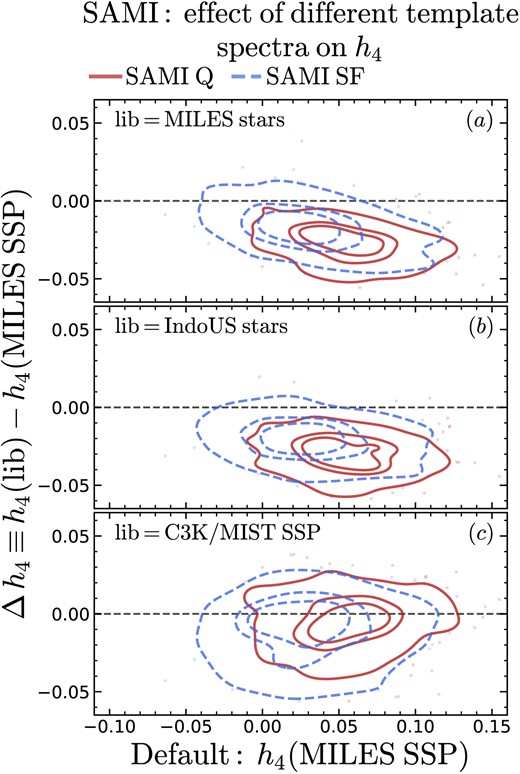
Effect of different input template spectra on the measured value of h4. The x-axis shows the default h4 measurement, obtained by modelling the galaxy spectra as a linear combination of SSP spectra from the MILES library. The y-axis shows the difference between alternative measurements of h4 and the default value. The solid red/dashed blue contours trace the 30th, 50th, and 90th percentiles of quiescent/star-forming SAMI galaxies. Panels a, b, and c show the effect of replacing the MILES SSP spectra with the MILES stellar spectra, the Indo-US stellar spectra, and the C3K/MIST SSP spectra. Stellar spectra tend to give lower values of h4, more so for quiescent galaxies; this translates into a smaller difference between star-forming and quiescent galaxies. We verified that the difference is still statistically significant, regardless of the library used.
APPENDIX C: AGE BIAS
As discussed in Section 3.2.2, for a meaningful comparison of h4 between star-forming and quiescent galaxies, we need to understand the effect of systematic differences in the spectra of these two classes of objects. To this end, we use two mock spectra, representing an idealized pair of a quiescent and a star-forming galaxy. For the quiescent galaxy, we assume a constant star formation rate SFR > 0 from the big bang until a look-back time of 10.25 Gyr (z ≈ 2), followed by SFR = 0. For the star-forming galaxy, we swap the intervals: SFR = 0 from the big bang until a look-back time of 10.25 Gyr, then constant SFR > 0. For each of these two spectra, we create a version with h4 = 0, and a version with h4 = 0.06, so we have four models in total. For each model, we then create 1000 random-noise realizations with S/N = 20 Å−1 and Gaussian noise. We then calculate |$\langle \Delta \, h_4 \rangle$|, the median offset between the measured and input values of h4. For h4 = 0, we find |$\langle \Delta \, h_4 \rangle = -0.0025\pm 0.0004$|10 and |$\langle \Delta \, h_4 \rangle = -0.0008\pm 0.0024$| for the quiescent and star-forming spectra. For h4 = 0.06, we find |$\langle \Delta \, h_4 \rangle = -0.0028\pm 0.0005$| and |$\langle \Delta \, h_4 \rangle = -0.0021\pm 0.0015$| for the quiescent and star-forming spectra. Even though some of these offsets are statistically significant, their magnitude is ×10 smaller than the maximum measurement uncertainties used for the quality cut (u(h4) < 0.05). As for the scatter, the standard deviation for the quiescent mocks is 0.010 (for h4 = 0) and 0.017 (for h4 = 0.06). These values are smaller than our threshold measurement uncertainties. For the star-forming mocks, the values are 0.075 (for h4 = 0) and 0.046 (for h4 = 0.06), which are comparable to our cut in the measurement uncertainties.
We remark here that real galaxies show clear evidence of correlation between the stellar population properties (age and chemical abundance) and kinematics. This is true not only in the Milky Way (e.g. Freeman & Bland-Hawthorn 2002; Nordström et al. 2004; Rix & Bovy 2013; Bland-Hawthorn & Gerhard 2016), but is well established in external galaxies too (e.g. Poci et al. 2019; Shetty et al. 2020, and Foster et al. 2023). For this reason, the tests we performed here are only a first-order approximation of the h4 bias between star-forming and quiescent galaxies.
APPENDIX D: SELECTION BIAS AGAINST LOW-MASS LEGA-C STAR-FORMING GALAXIES
Our quality selection (Section 4.2) results high completeness, except for the LEGA-C star-forming subset (Section 4.3, Fig. 6f). Incompleteness is most severe below |$M_\star = 10^{11} \, \mathrm{M_\odot }$|. Based on the h4–M⋆ correlation, we expect that, if it were possible to include non-selected star-forming galaxies in our analysis, the difference between star-forming and quiescent galaxies would be even stronger.
However, we cannot exclude that star-forming galaxies that do not meet our quality cut may be biased in other properties in addition to M⋆; what if these biases were to act opposite to the M⋆ bias?
In Fig. D1, we show that – below |$10^{11} \, \mathrm{M_\odot }$| – selected and non-selected star-forming galaxies differ in both structure (panel a) and stellar populations/dust (panel b). In the first panel a, the distribution of Sérsic index n of non-selected galaxies (grey histogram) clearly peaks at n = 1, with a small tail to higher n’s; in contrast, selected star-forming galaxies (dashed blue histogram) peak at n = 1.5 and have a broader distribution; our selection is biased against low-concentration, discy systems. In panel b, the distribution of non-selected galaxies is bluer, and extends also to significantly redder objects; so our selection is biased against both the youngest and most dust-obscured star-forming galaxies. However, using PCCs (Section 5), we find that – after controlling for M⋆ – n correlates with h4 and U-V shows no independent correlation with h4. This means that – had we accounted for the bias against low-n galaxies – the reported differences between star-forming and quiescent galaxies would be even larger.
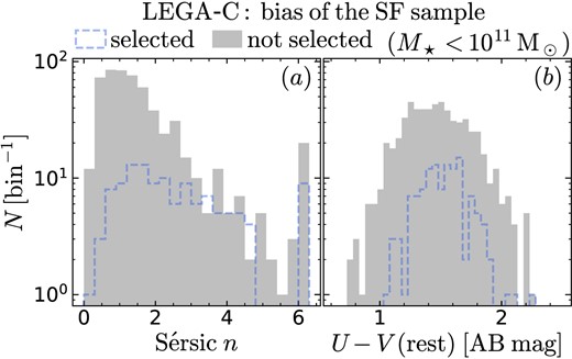
Below stellar mass |$10^{11} \, \mathrm{M_\odot }$|, the star-forming galaxies we select from LEGA-C differ systematically from their parent sample, in both structure (as highlighted by the Sérsic index n, panel a) and stellar-population properties (expressed by the rest-frame U-V colour, panel b). Based on the trends between h4 and M⋆, we expect non-selected star-forming galaxies to have lower h4 than selected star-forming galaxies; a higher completeness sample would probably reinforce our results. Differences in concentration and colour appear to be second-order effects, at best.
