


ABSTRACT
Type Ia supernovae (SNe Ia) arise from the thermonuclear explosion in binary systems involving carbon–oxygen white dwarfs (WDs). The pathway of WDs acquiring mass may produce circumstellar material (CSM). Observing SNe Ia within a few hours to a few days after the explosion can provide insight into the nature of CSM relating to the progenitor systems. In this paper, we propose a CSM model to investigate the effect of ejecta−CSM interaction on the early-time multiband light curves of SNe Ia. By varying the mass-loss history of the progenitor system, we apply the ejecta−CSM interaction model to fit the optical and ultraviolet (UV) photometric data of eight SNe Ia with early excess. The photometric data of SNe Ia in our sample can be well matched by our CSM model except for the UV-band light curve of iPTF14atg, indicating its early excess may not be due to the ejecta−CSM interaction. Meanwhile, the CSM interaction can generate synchrotron radiation from relativistic electrons in the shocked gas, making radio observations a distinctive probe of CSM. The radio luminosity based on our models suggests that positive detection of the radio signal is only possible within a few days after the explosion at higher radio frequencies (e.g. ∼250 GHz); at lower frequencies (e.g. ∼1.5 GHz), the detection is difficult. These models lead us to conclude that a multimessenger approach that involves UV, optical, and radio observations of SNe Ia a few days past explosion is needed to address many of the outstanding questions concerning the progenitor systems of SNe Ia.
1 INTRODUCTION
Type Ia supernovae (SNe Ia) are employed as the standardized candle in measuring cosmological distance through the luminosity–width relation (Riess et al. 1998; Perlmutter et al. 1999; Riess et al. 2007), although their progenitor systems are still unclear (e.g. Howell 2011; Maoz, Mannucci & Nelemans 2014) and they may have different progenitor populations even for spectroscopically normal ones (e.g. Wang et al. 2013, 2019). The conventional scenario is that SNe Ia are the results of the thermonuclear explosions of carbon–oxygen white dwarfs (WDs) whose masses approach the Chandrasekhar limit through merging with or accretion from a binary companion (e.g. Hillebrandt & Niemeyer 2000). In the merger scenario, the so-called double degenerate (DD) channel, the companion is another carbon–oxygen WD (Iben & Tutukov 1984; Webbink 1984), while in the single degenerate (SD) channel, a WD accretes matter from a main sequence, red giant, or helium star (Whelan & Iben 1973; Nomoto 1982). These two channels may both encounter difficulties when confronted with observations. The DD channel predicts a relatively high degree of polarization (Bulla et al. 2016), while the observed continuum polarization of SNe Ia is usually lower than 0.2 per cent (Wang, Wheeler & Höflich 1997; Wang & Wheeler 2008; Porter et al. 2016; Cikota et al. 2019; Yang et al. 2020). On the other hand, direct evidences of the SD channel have not been found from extensive observational efforts, such as the null detection of H/He emission lines in the nebular spectrum (Mattila et al. 2005; Lundqvist et al. 2013; Shappee et al. 2013; Maguire et al. 2016; Tucker et al. 2020), and the absence of supersoft X-ray signals as can be expected from the accretion process of progenitors (Nelemans et al. 2008; Kilpatrick et al. 2018).
Multiband observations within a few days after the explosion provide a powerful probe to investigate the physical origins of SNe Ia. In the SD channel, interaction with the companion can lead to radiations in the X-ray, ultraviolet (UV), and optical wavelengths several hours after the explosion in certain viewing angles (Kasen 2010; Maeda, Kutsuna & Shigeyama 2014). An early flux excess can also be produced if 56Ni is mixed to the outer layers of the ejecta due to hydrodynamic turbulence during the thermonuclear explosion (Magee et al. 2018, 2020), or if there is nuclear burning on the surface of the WD progenitor (Jiang et al. 2017, 2018; Maeda et al. 2018; Li et al. 2021; Magee et al. 2021). The interaction with circumstellar matter (CSM) can transform the kinetic energy of the ejecta into radiation and power the light curves of SNe with significant mass-loss history (Chevalier & Fransson 1994; Wood-Vasey, Wang & Aldering 2004; Svirski, Nakar & Sari 2012; Moriya et al. 2013; Takei & Shigeyama 2020). CSM interaction can also be the energy source of the first light-curve peak shown a few days after the explosion for some core-collapse SNe (Bersten et al. 2013; Piro 2015; Förster et al. 2018; Jin, Yoon & Blinnikov 2021). Likely, the possibility exists that the early flux excess of SNe Ia may originate from ejecta−CSM interaction (Moriya et al. 2023).
In recent decades, a large amount of photometric and spectroscopic observations of SNe Ia are available due to the rapid growth in time-domain surveys (e.g. Filippenko et al. 2001; Law et al. 2009; Kochanek et al. 2017; Graham et al. 2019), but data within the first few days after the explosion are still rare. This situation is mainly limited by the cadence of the SN survey programme, which is usually around 2 ∼ 3 d to cover as large a survey area as possible. With recent wide-field SN survey programmes (Law et al. 2009; Tonry et al. 2018; Dekany et al. 2020), more and more early signals of SNe Ia have been captured, such as the spectroscopic normal ones [e.g. SN 2011fe (Nugent et al. 2011), SN 2012cg (Marion et al. 2016), SN 2017cbv (Hosseinzadeh et al. 2017; Wang et al. 2020), SN 2018oh (Dimitriadis et al. 2019; Li et al. 2019), SN 2019np (Sai et al. 2022), and SN 2021aefx (Ashall et al. 2022; Hosseinzadeh et al. 2022)], subluminous 2002es-like ones [e.g. iPTF14atg (Cao et al. 2015) and SN 2019yvq (Miller et al. 2020a; Burke et al. 2021)], and the super-Chandrasekhar explosion [e.g. SN 2020hvf (Jiang et al. 2021)].
The above nine SNe Ia also constitute the sample of this paper. The first detection of SN 2011fe is just several hours after its explosion, and such early photometric data in consistence with a tα law constrain the radius of the progenitor to that of a WD (Li et al. 2011; Nugent et al. 2011; Bloom et al. 2012). The other eight SNe Ia are revisited in this paper because they show apparent flux excess during their early phases compared with the light curve of typical objects such as SN 2011fe. In particular, SN 2017cbv exhibits apparent blue excess in its early phases. This flux excess may be generated from the decay of 56Ni mixed in the outer layers of the ejecta (Magee & Maguire 2020), 56Ni produced at the surface layers due to a helium detonation (Maeda et al. 2018), the interaction with the companion star (Hosseinzadeh et al. 2017), or ejecta−CSM interaction. For the companion interaction scenario, the predicted large amount of UV radiation is not supported by observations (Hosseinzadeh et al. 2017). Besides, the predicted H/He emission lines in the nebular spectra relating to the SD channel are not observed for SN 2017cbv (Sand et al. 2018).
In this paper, we revisited the influence of CSM interaction on the early multiband light curves of SNe Ia, since the popular channels of progenitor systems may generate CSM through the processes involving mass accretion/excretion, stellar wind, or nova explosions. Section 2 describes the early flux excess of the eight revisited SNe Ia in our sample. In Section 3, two models of ejecta−CSM interaction are introduced. The fits to the optical and UV luminosity are shown in Section 4. We show the radio radiation from the relativistic electrons generated by the ejecta−CSM interaction in Section 5. The conclusions are given in Section 6.
2 THE EARLY EXCESS OF THERMONUCLEAR SUPERNOVAE
Several recent studies have modelled the early-phase observations of SNe Ia through their UV properties (Brown et al. 2012a), optical rises (Jiang et al. 2020; Miller et al. 2020b; Fausnaugh et al. 2021), and colour evolutions (Bulla et al. 2020). In this paper, we focus on the ejecta−CSM interaction to model eight SNe Ia with the strongest evidences of early flux excess. Among them, SN 2012cg (Marion et al. 2016), iPTF14atg (Cao et al. 2015), and SN 2019yvq (Miller et al. 2020a) show an initial declining flux excess in the UV bands which may be related to the ejecta−CSM interaction. The early flux excesses of SN 2017cbv (Hosseinzadeh et al. 2017; Maeda et al. 2018; Magee & Maguire 2020), SN 2018oh (Dimitriadis et al. 2019; Levanon & Soker 2019), SN 2019np (Sai et al. 2022), and SN 2021aefx (Ashall et al. 2022; Hosseinzadeh et al. 2022) are still under debate, while SN 2020hvf (Jiang et al. 2021) seems to show optical bumps within the first day since the discovery which is consistent with the expectations from ejecta−CSM interaction. SN 2016jhr also has early observations showing flux excess compared to typical normal SNe Ia, but it is not in our sample since its early flash is likely to be triggered by a helium detonation on the surface of the WD (Jiang et al. 2017).
The optical light curves of SNe Ia in our studies have different photometric systems, including the Sloan Digital Sky Survey photometry, the Johnson–Cousins UBVRI system, the Kepler filter (SN 2018oh), and no-filter observations (SN 2020hvf). All the UV-band light curves are from the Swift satellite. Therefore, we adopt the optical luminosity (Lopti) to characterize the early excess of the eight SNe Ia in our study to reduce the influence of the magnitude systems among the observations of SNe Ia, and we adopt the UV-band luminosity (LUV) to represent the early-phase evolution in UV bands. The Lopti defined in this paper is the integration of the blackbody spectrum fitted by the multiband photometric data from 4000 to 8000 Å. As shown in Fig. 1, the blackbody spectrum is a favourable profile fitting the early-time multiband photometric data of SNe Ia. For iPTF14atg, SN 2018oh, and SN 2020hvf, the optical multiband observations are absent in the duration of early excess, and the observational band is PTFr band (iPTF14atg), Kepler filter (SN 2018oh), or no-filter (SN 2020hvf), respectively. Therefore, we adopted the shape of the single-band light curve as the shape of the Lopti curve during the flux-excess phases for these three SNe Ia. We then shifted the single-band flux to the scale of the corresponding optical luminosity with the overlap between the single-band data and multiband data to obtain the Lopti curve.
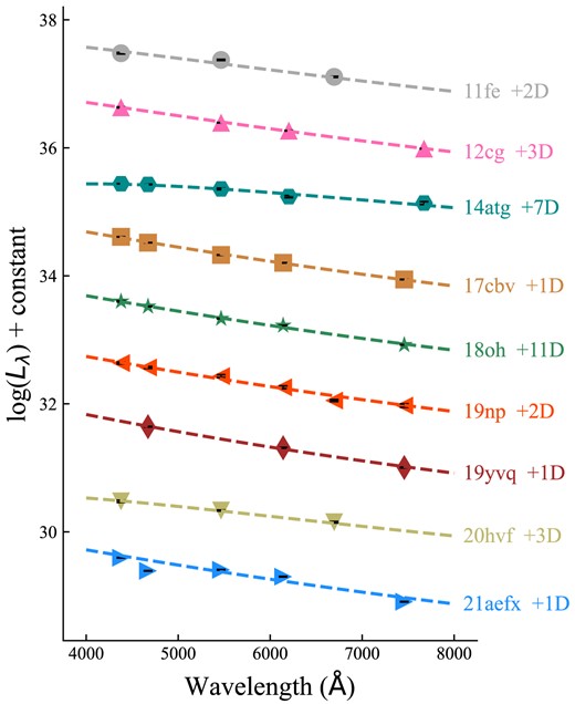
The symbols are the early-phase luminosity of the revisited SNe Ia at each optical band’s efficient wavelength (Lλ). The dashed lines are the corresponding blackbody spectrum fits. The phases listed in the figure correspond to the explosion of each SN Ia.
The optical photometric data of SNe Ia are de-reddened from the extinction of the Milky Way and host galaxies. The colour excess E(B − V), the total-to-selective extinction ratio (RV), and the luminosity distance of the SNe Ia are all from their respective references. Note that we adopted 12.3 Mpc as the distance of SN 2017cbv derived from Sand et al. (2018). A similar distance to SN 2017cbv is also adopted in several other studies (Wee et al. 2018; Burns et al. 2020; Wang et al. 2020). Fig. 2 displays the normalized Lopti curves of the eight SNe Ia, together with SN 2011fe for comparison. We adopt a modified fireball model to fit the early-time luminosity of SNe Ia, in which Lopti ∝ tα, where t is the time since the explosion, and α is a power-law index (Riess et al. 1999; Ganeshalingam, Li & Filippenko 2011). Note that the ‘explosion time’ defined in our paper is likely the first-light time due to the possible existence of a so-called ‘dark phase’ between the explosion epoch and the time of the first time for SNe Ia. The index α is not fixed to be 2.0 owning to the possible evolution of expansion velocity or fireball temperature during the early time. Besides, we fitted the early-time luminosity curve using the epochs from +5 to +8 d since the explosion due to the early excess of the revisited SNe Ia in our study. The ratio between the optical luminosity at +8 d since the explosion and the peak luminosity is about 0.4, consistent with the choice in Miller et al. (2020b). The early-time Lopti curve of SNe Ia satisfies the tα law with the index α ∼ 2.0, which is consistent with previous results (Pereira et al. 2013; Firth et al. 2015; Zhang et al. 2016). The early-time optical excesses of the eight SNe Ia over the tα law (Lopti,excess) are shown in the lower panel of Fig. 2, and it can be roughly described by two quantities, the maximum of Lopti,excess (|$L_{\text{opti, excess}}^{\text{max}}$|) and the rising time (Trise) of Lopti,excess since the explosion. For simplicity, the values of |$L_{\text{opti, excess}}^{\text{max}}$| and Trise are just from the corresponding data point without any process like the Gaussian process fit or smooth process. These two quantities can provide a preliminary diagnosis of our ejecta−CSM interaction model.
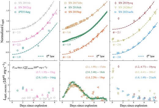
Upper panels: the symbols represent the normalized optical luminosity (Lopti) of SN 2011fe (Zhang et al. 2016), which has no early excess and the eight SNe Ia with early excess, including SN 2012cg (Marion et al. 2016), iPTF14atg (Cao et al. 2015), SN 2017cbv (Hosseinzadeh et al. 2017; Wang et al. 2020), SN 2018oh (Dimitriadis et al. 2019; Li et al. 2019), SN 2019np (Sai et al. 2022), SN 2019yvq (Miller et al. 2020a; Burke et al. 2021), SN 2020hvf (Jiang et al. 2021), and SN 2021aefx (Ashall et al. 2022; Hosseinzadeh et al. 2022). Lopti is the integration of the blackbody spectrum from 4000 to 8000 Å fitted by their multiband photometric data except for iPTF14atg, SN 2018oh, and SN 2020hvf due to the lack of multiband observations during their early phases (see Section 2 for more details). The dashed lines show the tα fit to the photometric data of each SN Ia. The lower panels show the differences between the Lopti of each SN Ia and the tα law derived from the SN Ia itself. For comparison, we list the rising time (Trise) and the peak of the Lopti,excess (|$L^{\text{max}}_{\text{opti, excess}}$|) of the eight SNe Ia with early excess.
The same process is also applied to generate the early-phase UV-band light curves of each SN Ia with extinction corrections using the same RV and E(B − V) as for Lopti. Fig. 3 shows the normalized LUV of SNe Ia. Similarly, a tα law of LUV is generated from the observed data of SN 2011fe, with α = 2.3, 2.4, or 2.0 for UVW1, UVW2, or UVM2 band, which are consistent with the result reported in Marion et al. (2016). Note that the template of the UV-band light curve is from the smoothed curve of SN 2011fe rather than the fitted tα law of SN 2011fe, and the difference between the smoothed curve and the tα law is minimal within a few days since the explosion as shown in Fig. 3. Comparing Figs 2 and 3, SN 2012cg, iPTF14atg, SN 2017cbv, SN 2019np, SN 2019yvq, and SN 2021aefx all have early-time multiband observations (from optical to UV bands), and all show significant excess over the tα law, while the UV-band coverage is absent for SN 2018oh and SN 2020hvf during the phases corresponding to the early optical excess.
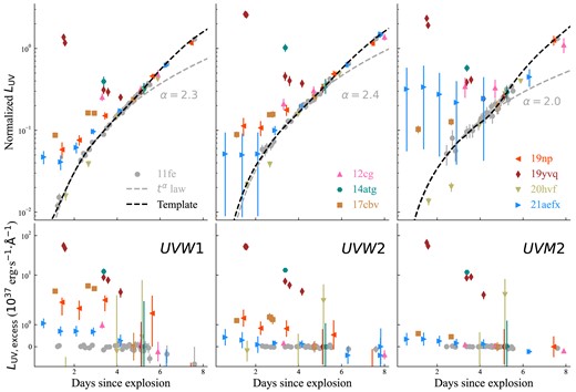
Be similar with Fig. 2 but for the luminosity of UVW1 band, UVW2 band, and UVM2 band, respectively. The dashed grey lines are the tα fit to the photometric data of SN 2011fe. The dashed black lines are smooth to the photometric data of SN 2011fe and are regarded as the template of UV-band luminosity in our study. The lower panel shows the differences between the LUV of each SN Ia and the template of LUV derived from SN 2011fe. The references of the photometric data are same as shown in Fig. 2 except for SN 2011fe (Brown et al. 2012b).
With the definition of both Lopti and LUVW1, it is straightforward to examine the possible CSM interaction origin of the early excess emission in SNe Ia. We will compare |$L_{\text{opti, excess}}^{\text{max}}$| and Trise of the revisited SNe Ia with our CSM model covering a broad range of model parameters to give a quick look of whether our CSM model is reasonable for the early excess of SNe Ia. We then fit the early excess of Lopti curves and predict the related LUVW1 curves. The model parameters from these well-fitted models are employed to predict further the radio radiations related to the ejecta−CSM interactions of these SNe Ia.
3 THE CSM INTERACTION MODEL
The ejecta−CSM interaction has been studied previously for SNe (e.g. Chevalier 1982a; Chevalier & Fransson 1994; Wood-Vasey et al. 2004; Moriya et al. 2013). The CSM density (ρCSM) considered in this study follows the expression |$\rho _{\text{csm}} = \dot{M}_{\text{w}}/(4\pi R^2 v_{\rm w})$|, where R is the distance from the SN, |$\dot{M}_{\text{w}}$| is the mass-loss rate of CSM, and vw is the wind speed. We adopt vw = 10 km s−1 in the study. For a constant |$\dot{M}_{\text{w}}$|, the total CSM mass MCSM is equal to |$(R_{\text{out}}-R_{\text{in}})\dot{M}_{\text{w}}/v_{\rm w}$| with Rin and Rout being the inner and outer boundaries of the CSM, respectively. In general, Rin is related to the position of the surface of the progenitor and we set Rin to zero, while Rout is assumed to vary from 1011 to 1016 cm in our study.
The velocity of SN ejecta (vej) satisfies vej = R/t as expected from a homologous expansion, where t is the time since SN explosion. The density (ρej) of the ejecta follows the power-law profile of ρej ∝ R−δ and ρej ∝ R−n for regions interior and exterior of a transition velocity vt (Matzner & McKee 1999; Kasen 2010), respectively. The indices n and δ are equal to 10.0 and 0.5 as expected from self-similar solutions. The transition velocity vt is formulated by the SN kinetic energy Eej and ejecta mass Mej as |$v_\mathrm{ t} = [\frac{2(5-\delta)(n-5)E_{\text{ej}}}{(3-\delta)(n-3)M_{\text{ej}}}]^{1/2}$| (Moriya et al. 2013). The value of vt is about 1.2 × 10⁴ km s−1 assuming Eej = 1.5 × 1051 erg and Mej = 1.4 M⊙ (Maeda et al. 2018).
3.1 Model_sh
The first scenario considered in our study, named Model_sh, has the characteristic parameters of Rout ∼ 1012 cm, |$\dot{M}_{\text{w}}\sim 10^{-1}\ \text{M}_{\odot }\, \text{yr}^{-1}$|, and the corresponding total CSM mass MCSM ∼ 0.003 M⊙. The duration of CSM interaction in the Model_sh is less than an hour, and the interaction process can be regarded as a shock breakout, which results in a thin shell expanding with velocity Vsh at a distance Rsh and a shell thickness ΔRsh. We adopt ΔRsh/Rsh ∼ 0.2 in the Model_sh, which is different from Maeda et al. (2018), but is consistent with the results in Chevalier (1982a). The Rsh evolves as Rsh = Rout + Vsht. Vsh is determined by the equation assuming that the mass of the shocked ejecta is equal to the total mass of the CSM such that |$\int _{V_{\text{sh}}}^{\infty }4\pi (vt)^2\rho _{\text{ej}}t\mathrm{d}v = M_{\text{csm}}$| (Maeda et al. 2018). The bolometric luminosity (L) from this adiabatically expanding shell can be solved by the first law of thermodynamics as |$L\propto \exp (-\frac{t_ht+t^2/2}{t_ht_d(0)})$|, where th = Rout/Vsh and td(0) is the diffusion time-scale when t = 0 (Maeda et al. 2018). The observed multiband light curves can be generated with the assumption of blackbody radiation. Note that the bolometric luminosity is monotonically decreasing with time, while the light curve of a certain waveband has a unimodal structure. Thus, the predicted flux contributions by Model_sh allow calculations of quantities such as the maximum optical luminosity of the ejecta−CSM interaction and the rising time since the explosion.
3.2 Model_ext
The interaction with extended CSM cannot be simplified to the shock breakout process since the interaction can last more than a few days. A similar situation may happen for SNe Ia, because the mass-loss history for the progenitor may be long enough to generate CSM with an extended distribution. Based on this picture, we consider the scenario Model_ext, which has a more extended CSM (e.g. the outer boundary of CSM is ∼1015 cm), and we assume that the unshocked CSM is optically thin. The evolution of Rsh and Vsh for the shocked CSM satisfies the conservation of momentum as follows,
where Msh is the total mass of the shocked ejecta and CSM. In Model_ext, we only consider the interaction process during the first few days after the explosion, and |$\dot{M}_{\text{w}}$| is basically less than 10−4 M⊙ yr−1 as has been constrained by radio or X-ray observations of SNe Ia (Panagia et al. 2006; Russell & Immler 2012; Chomiuk et al. 2016; Lundqvist et al. 2020). Thus, the shocked SN ejecta is always confined inside the exterior part of the ejecta with vej > vt. With the solution of the kinetic evolution, the corresponding bolometric luminosity L is given by the power of the shocked CSM with a conversion efficiency ϵ as |$L = \frac{\epsilon }{2}\dot{M}_{\text{w}}V_{\text{sh}}^3$|, where ϵ = 0.15 in our simulations in consistence with previous studies (Chevalier 1982a; Moriya et al. 2013). On the other hand, one important quantity in the Model_ext is |$\dot{M}_{\text{w}}(R)$| which is a function of the distance R as given below,
As shown in equation (2), |$\dot{M}_{\text{w}}(R)$| increases to |$\dot{M}_{\text{w}}(0)$| within the distance of R1 relating to an index of n1. |$\dot{M}_{\text{w}}(R)$| is equal to a constant |$\dot{M}_{\text{w}}(0)$| between R1 and R2. |$\dot{M}_{\text{w}}(R)$| decreases to zero from R2 to R3 with an index of n2. CSM could be ignored for a distance larger than R3. The range of parameters n1 and n2 is from 0.0 to 3.0.
Therefore, the observed light curves for Model_ext can be numerically solved based on equation (1). As a simplified situation with a constant |$\dot{M}_{\text{w}}(R)$|, Moriya et al. (2013) acquired the integrated formula of the luminosity curve of CSM interaction. We compared the evolution of Rsh between the integrated formula from Moriya et al. (2013) and our numerical solutions with a constant |$\dot{M}_{\text{w}}(R)$| as shown in Fig. 4, which demonstrate the validity of our numerical procedure. Note that our ejecta−CSM interaction model is one-dimensional assuming a spherical explosion and spherical distribution of CSM. The polarimetric observations suggest the explosion of SNe Ia is approximately spherical (Wang & Wheeler 2008), and the distribution of CSM is also spherical if the mass-loss process is isotropic. However, the interaction with an aspherical CSM may exist, which may generate different luminosity curves and possible polarimetric signals.
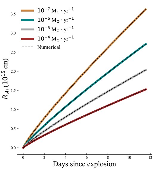
The orange, cyan, grey, and red solid lines show the evolution of the radii of the shocked CSM shell (Rsh) calculated by the formula in Moriya et al. (2013) with |$\dot{M}_{\text{w}}$| of 10−7, 10−6, 10−5, and 10−4 M⊙ yr−1, respectively. The dashed black lines are the evolution of Rsh solved numerically by our CSM model.
3.3 Dusty CSM
Assuming any typical gas-to-dust ratios, we introduce the effect of dusty CSM on the UV-band light curves. As estimated in Amanullah & Goobar (2011), the pre-existing circumstellar dust within ∼1016 cm would be destroyed by the peak luminosity of SNe Ia. Consequently, the evaporation radius of circumstellar dust would rapidly increase as the increase of bolometric luminosity soon after the explosion. Taking SN 2011fe as an example, the bolometric luminosity at +1, +2, and +4 d since the explosion is about 3.5 × 1040, 2.0 × 1041, and 1.4 × 1042 erg s−1, respectively. With the assumption of the peak bolometric luminosity of 1043 erg s−1 and a rough estimation of the evaporation radius from Amanullah & Goobar (2011), the hypothesized evaporation radii for SN 2011fe at +1, +2, and +4 d since the explosion is about 6 × 10¹⁴, 1.4 × 10¹⁵, and 3.7 × 1015 cm, respectively. However, time-dependent dust destruction is a complicated process during the early phase of SNe Ia. Nevertheless, we only consider the dusty CSM in the Model_ext rather than in Model_sh due to the difference in characteristic distances. To investigate the absorption and scattering from circumstellar dust, we consider a simple dust model in which the chemical composition is just silicate with a typical size of |$0.05\ \mu \text{m}$|, indicating that the dust extinction is more significant in UV bands than in the optical.
For simplicity, we assume a spherical distribution of the dust within an inner boundary of 1 × 1015 cm and an outer boundary of 5 × 1015 cm. The optical depth in B-band is adopted as 0.15, the corresponding optical depth in UVW1 band is 1.1, and the averaged optical depth from 4000 to 8000 Å is about 0.07. Thus, the radiative transfer process in dusty CSM for optical bands is ignored in this paper. Assuming the same wind velocity (10 km s−1), the mass-loss rate of the dust is about 1 × 10⁻⁸ M⊙ yr−1, which is about 10−2 times of the typical value of |$\dot{M}_{\text{w}}(0)$| (∼10−6 M⊙ yr−1) in the Model_ext as illustrated in Fig. 5. We assume that the inner boundary of circumstellar dust increases linearly from 1 × 1015 cm at the initial state to 5 × 1015 cm at +4 d since the explosion, which is consistent with the above discussion of the hypothesized evaporation radius relating to the early-phase bolometric luminosity of SN 2011fe. The time-dependent dust destruction makes the radiative transfer in the dusty CSM a dynamic process. We incorporated this dynamic process in our Monte Carlo radiative transfer programme in Hu, Wang & Wang (2022b) to solve for the UV fluxes in dusty CSM.
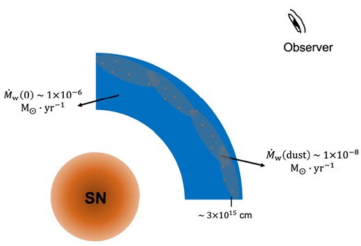
The illustration of the configuration of Model_ext with dusty CSM around SNe Ia modelling UV-band light curves. The grey area with grey dots is where the dust exists. The mass-loss rate of the dust (|$\dot{M}_{\text{w}}(\text{dust})$|) is related to B −band optical depth of 0.15 and the dust distance of 3 × 1015 cm. For comparison, |$\dot{M}_{\text{w}}(0)$| with a characteristic value of around 1 × 10⁻⁶ M⊙ yr−1 is also shown in the figure.
4 FITTING THE EARLY EXCESS EMISSION WITH CSM INTERACTION
Fig. 6 displays the predicted rising time of the optical excess versus the maximum of the optical excess for Model_sh and Model_ext with different parameter configurations. For Model_sh, Rout is set to 1012, 1013, and 5 × 1013 cm, and |$\dot{M}_{\text{w}}$| is set to from 0.001 to 1.0 M⊙ yr−1. The corresponding total CSM mass is in the range of 1.6 × 10⁻⁵–0.16 M⊙. For Model_ext, although R1, R2, R3, and |$\dot{M}_{\text{w}}(0)$| are all free parameters, R2 and |$\dot{M}_{\text{w}}(0)$| can significantly influence the flux relating to the ejecta−CSM interaction. The ranges of parameter R2 considered here is set to 2 × 10¹⁴, 1015, and 5 × 1015 cm, and |$\dot{M}_{\text{w}}(0)$| varies from 10−7 to 10−4 M⊙ yr−1. It is clearly shown that Model_sh in each parameter grid has the characteristics of a very short duration, which is contradictory to the early flux excess of the revisited SNe Ia in this paper except for SN 2020hvf. Meanwhile, Model_ext with certain parameters can fit the early optical excess of SNe Ia satisfactorily. However, combining the photometric data of optical and UV bands may examine the hypothesis that the early excess arises from the ejecta−CSM interaction.
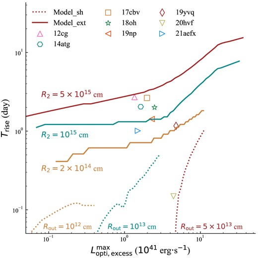
The lines are the predicted rising time of the optical excess versus the maximum of the optical excess for Model_sh (dotted lines) with Rout of 1012 cm (yellow), 1013 cm (cyan), and 5 × 1013 cm (red), and for Model_ext (solid lines) with R2 of 2 × 1014 cm (yellow), 1015 cm (cyan), and 5 × 1015 cm (red), respectively. For each line of Model_sh, the |$\dot{M}_{\text{w}}$| ranges from 0.001 to 1.0 M⊙ yr−1, and the value of |$\dot{M}_{\text{w}}(0)$| for each line of Model_ext ranges from 10−7–10−4 M⊙ yr−1. For simplicity, we set R1 = 0.4 × R2 and R3 = 2.0 × R2. All the symbols are the Trise and |$L_{\text{opti, excess}}^{\text{max}}$| calculated from the luminosity residual shown in the lower panel of Fig. 2 for the eight revisited SNe Ia in this paper.
We adopt Model_sh to fit the early-time optical excess of SN 2020hvf (Rout = 3 × 1013 cm, MCSM = 0.05 M⊙) and Model_ext for the rest seven SNe Ia with the parameter values shown in Table 1. The fitted optical luminosity curves and the predicted UVW1-band luminosity are shown in Fig. 7. The result clearly suggests that ejecta−CSM interaction can explain the early excess in the optical band of SNe Ia, and the total mass of CSM is at the level of about 10−4 M⊙ in agreement with the observations on the non-detection of H emission lines in the nebular spectrum (e.g. Lundqvist et al. 2013; Maguire et al. 2016; Sand et al. 2018; Tucker et al. 2020).
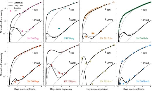
The results of our CSM model fitting the early excess of the eight revisited SNe Ia in this paper. Model_sh is used to fit the signal of SN 2020hvf, and Model_ext is used for the rest seven SNe Ia. For each panel, the dashed grey lines are the normalized luminosity template generated from tα law (Lopti) or smoothing process (LUVW1). The solid black lines are the fitted luminosity curves from our CSM model without considering the existence of dust, while the dotted black lines are the predicted LUVW1 curves with the extinction and scattering of circumstellar dust. All the symbols are the data of each SN Ia with the same colour and shape as shown in Fig. 2.
Here are the parameter values of Model_ext for fitting the early flux excess of SNe Ia except for SN 2020hvf. The unit of parameters R1, R2, and R3 is 1014 cm, and that of |$\dot{M}_{\text{w}}(0)$| is 10−6 M⊙ yr−1. MCSM is the total mass of CSM integrated to the distance of R3.
| SNe | R1 | R2 | R3 | |$\dot{M}_{\text{w}}(0)$| | MCSM/10−4 M⊙ |
|---|---|---|---|---|---|
| 12cg | 6 | 8 | 20 | 3.0 | 0.52 |
| 14atg | 7 | 10 | 30 | 3.0 | 1.2 |
| 17cbv | 3 | 6 | 16 | 3.0 | 0.56 |
| 18oh | 5 | 10 | 25 | 4.0 | 1.1 |
| 19np | 5 | 10 | 20 | 3.5 | 0.87 |
| 19yvq | 1.5 | 3 | 15 | 35.0 | 4.3 |
| 21aefx | 3 | 8 | 18 | 1.5 | 0.37 |
However, the great deviation of the predictions on UVW1-band luminosity suggests that the early-time excess of iPTF14atg may not be generated from the ejecta−CSM interaction but the ejecta−companion interaction since the ejecta–companion interaction can produce much higher temperature and hence more luminous UV-band radiation (Kasen 2010; Cao et al. 2015; Marion et al. 2016). As the discussion in Jiang et al. (2021), the early excess of SN 2020hvf is highly possible to be generated from the CSM interaction process for its short duration of the optical flash. The values of parameter Rout and MCSM in fitting SN 2020hvf are slightly different from that in Jiang et al. (2021) due to the simplification of Lopti for SN 2020hvf in this paper. The fitting Lopti of SN 2018oh can only indicate that the ejecta−CSM interaction may be one of possible origination due to the lack of the early-time UV-band observations. For SNe 2012cg, 2017cbv, 2019np, and 2021aefx, the predicted LUVW1 is consistent with the observed data considering the extinction from dusty CSM. A further diagnosis from radio observations is discussed in Section 5.
5 THE RADIO RADIATION FROM CSM INTERACTION
An evident phenomenon of CSM interaction is the radio radiation emitted by the relativistic electrons. Although almost all the radio observations of spectroscopic normal SNe Ia can only provide an upper limit, the radio radiation from ejecta−CSM interaction has important potential in distinguishing the various scenarios. The theory of the radio radiation from CSM interaction has been well established (Chevalier 1982b, 1998; Björnsson & Lundqvist 2014; Pérez-Torres et al. 2014; Lundqvist et al. 2020), and here we apply this theory to SNe Ia with ejecta−CSM interaction soon after explosion.
5.1 The synchrotron radiation
A reasonable assumption is that the relativistic electrons produced by the ejecta−CSM interaction follow a power-law distribution, dN/dE = N0E−p, where N and N0 are the number density of the relativistic electrons and a scaling parameter, respectively. E = γmec2 is the energy of the electrons with γ being the Lorentz factor. The corresponding synchrotron emission coefficient (jν) is proportional to a declining power law of the frequency of the radiated photons, jν ∝ ν−α, where the parameter α is equal to (p − 1)/2. We adopt α = 1 and p = 3 in this study.
5.2 The synchrotron self-absorption
The effect of the synchrotron self-absorption (SSA) cannot be ignored because N0 and the magnetic field (B) might be large enough to make the shocked area optically thick for the radio radiation. Assuming a uniform opacity distribution with the path length Δs, the optical depth τν is expressed as τν = κνΔs, where κν is the absorption coefficient and κν = κ0(p)N0B(p + 2)/2ν−(p + 4)/2, where κ0(p) is a constant (=5.5 × 1026 for p = 3). The intensity (Iν) is acquired by an integral as |$I_{\nu } = \int _0^{\Delta s} j_{\nu }\exp (-\kappa _{\nu }s)\mathrm{d}s = \frac{j_{\nu }}{\kappa _{\nu }}(1-\exp (-\tau _{\nu }))$|. Thus, the source function (Sν = jν/κν) is proportional to ν5/2.
For the simplicity of calculating Sν, we introduce a characteristic frequency νabs, which has a corresponding optical depth τabs ∼ 1. This directly leads to τν = (ν/νabs)−(p + 4)/2. Besides, we can define a frequency νpeak as |$I_{\nu _{\text{peak}}}\equiv 2kT_{\text{bright}}(\nu _{\text{peak}}/c)^2$|, where k is the Boltzmann constant and Tbright is the brightness temperature. Thus, the intensity of any frequency can be formulated by |$I_{\nu } = \frac{S_{\nu }}{S_{\nu _{\text{peak}}}}\frac{1-\exp (-\tau _{\nu })}{1-\exp (-\tau _{\nu _{\text{peak}}})}I_{\nu _{\text{peak}}}$|. After proper arrangement, the formula is as follows,
where x = νpeak/νabs and f(x) = x1/2[1 − exp (−x−(p + 4)/2)]. Based on the equation (12) in Björnsson & Lundqvist (2014), x ≈ 1.137 for p = 3. With τabs ∼ 1, we can get that νabs = (Δsκ0(p)N0B(p + 2)/2)2/(p + 4).
5.3 The radio luminosity from CSM interaction
The kinetic evolution of the shocked shell can be constrained from Model_ext with the assumption of ΔRsh = 0.2Rsh. Following the results in Pérez-Torres et al. (2014), we assume that γmin ≈ 1.64[Vsh/(70 000 km s−1)]2 and γmin ≥ 1. We then have |$N_0 = (p-2)\epsilon _{\text{rel}}u_{\text{th}}E_{\text{min}}^{p-2}$| by integrating the power-law distribution of the relativistic electrons, where |$u_{\text{th}} = (9/8)\rho _{\text{csm}}V_{\text{sh}}^2$| is the thermal energy density and ϵrel is the ratio of the energy density of the relativistic electrons and uth. Besides, the magnetic field is determined by B2/(8π) = ϵButh, where ϵB is the ratio of the magnetic energy density and uth. We set ϵrel = 0.1 and ϵB = 0.01 in our simulations (Pérez-Torres et al. 2014).
Assuming that the shocked shell is homogeneous, the intensity along the line of sight is a function of the polar angle due to the path length. We define a parameter h = sin θ, where θ is the polar angle with respect to the direction of the line of sight. For h = 0, we denote νabs = νabs,0, τν = τν,0, and |$\tau _{\nu _{\text{abs}}} = \tau _{\nu _{\text{abs,0}}} = 1$|. For 0 ≥ h ≥ 1, τν(h) = ξhτν,0, where ξh = Δs(h)/(2ΔRsh). Thus, Iν(h) can be directly derived from equation (3) by replacing νabs and τν with νabs,0 and τν(h), respectively. The luminosity Lν is the integration over h as |$L_{\nu } = 8\pi ^2R_{\text{sh}}^2\int _0^1I_{\nu }(h)h\mathrm{d}h$|. We then define a factor ϑ = Lν/Lν,0, where |$L_{\nu ,0} = 4\pi ^2R_{\text{sh}}^2I_{\nu }(0)$|. Thus, we can get the observed luminosity as,
where |$L_0 = \frac{8\pi ^2kT_{\text{bright}}}{c^2f(x)}R_{\text{sh}}^2\vartheta$|. For optically thin or thick shell, equation (4) is reduced to |$L_{\nu } = L_0\nu _{\text{abs,0}}^{(p+3)/2}\nu ^{-(p-1)/2}$| or |$L_{\nu } = L_0\nu ^{5/2}/\nu _{\text{abs,0}}^{1/2}$|, respectively. In our simulations, the optical depth τν,0 evolves with time during the process of ejecta−CSM interaction.
5.4 The predicted radio luminosity by the Model_ext
Here, we compare the predicted radio radiation from the ejecta−CSM interaction process with the early-phase radio observations of SNe Ia. For SNe 2012cg, 2019np, and 2021aefx, the predicted radio radiation is compared with their observed upper limits of radio fluxes. For SNe 2017cbv, 2018oh, and 2019yvq, the predicted radio radiation is compared with the observational data of normal SNe Ia from Chomiuk et al. (2016) due to the lack of the early-time radio observations of these three events. The predicted curves of radio luminosity for the low frequencies (e.g. 1.5, 4.0, and 5.5 GHz) and for the high frequency (250 GHz) are shown in Fig. 8 with the same CSM parameter values as shown in Table 1. At the beginning of the ejecta−CSM interaction, the optical depth of radio bands is so large due to SSA that the radio luminosity at low frequencies is relatively low. As the shocked shell travels outwards, the CSM density rapidly decreases, resulting in a sharp decrease of the radio radiation for both high and low frequencies. The predicted radio luminosity is compared with the observations of SNe Ia excluding the peculiar ones such as Iax, 02es-like, Ca-rich, super-Chandrasekhar, and Ia–CSM in Fig. 8. The predicted curves are below the upper limits of radio observations, except for SNe 2011fe and 2014J. This implies that even with the revisited SNe Ia, which show obvious early light curve bumps, the existing observations are not sensitive enough to reveal the underlying CSM interaction. The progenitor mass-loss rate soon before the explosion is even more tenuous for those SNe with detection limits lower than the predicted radio flux. For instance, the upper limit of the mass-loss rate of SN 2011fe and SN 2014J is about 1 × 10⁻¹⁰ M⊙ yr−1 from our calculation, which is a little bit smaller than the upper limit from Chomiuk et al. (2016) due to the configuration setting of CSM interaction models.
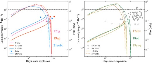
The left-hand panel: the symbols are the observed upper limits of radio fluxes of SN 2012cg (pink, 4.0 GHz), SN 2019np (purple, 1.5 GHz), and SN 2021aefx (blue, 5.5 GHz), respectively. The solid lines are the predicted radio luminosities derived from the ejecta–CSM interaction with the same parameter values shown in Table 1. The right-hand panel displays the predicted radio radiation in 1.5 GHz for SNe 2017cbv (solid orange line), 2018oh (solid green line), and 2019yvq (solid yellow line), comparing with the upper limits of radio fluxes of SNe Ia (filled grey circles) from the tables in Chomiuk et al. (2016), including the highlighted SNe 2011fe (open circles) and 2014J (open diamond) and excluding the peculiar ones such as Iax, 02es-like, Ca-rich, super-Chandrasekhar, and Ia–CSM. The dashed lines in both panels are the corresponding radiation curves in 250 GHz. The corresponding radio flux scale assuming a distance of 20 Mpc, is displayed on the vertical axis on the right-hand side. For comparison, the horizontal dotted line is the sensitivity of ALMA with an integration time of 300 s. The SSA effect is significant, especially at lower frequencies, and poses a challenge to radio observations at frequencies below ∼10 GHz.
Besides, the radio light curves shown in Fig. 8 suggest that the radio observation at higher frequency (e.g. ∼250 GHz) is several orders of magnitude stronger than at lower frequency (e.g. ∼1.5 GHz). However, the biggest constraint is that the radio observations must be triggered within a few days after the explosion of SNe Ia with early optical excess. Such high-frequency observations may be achievable by the Atacama Large Millimeter/submillimeter Array (ALMA) telescope. As shown in Fig. 8, the luminosity of 250 GHz can exceed about 1027 erg s−1 Hz−1 during +1 to +5 d with respect to the explosion. The corresponding flux is about 10.0 mJy at a distance of about 20 Mpc, which happens to be within the sensitivity of the ALMA. It is critical to discover nearby SNe Ia within one or two days after the explosion and triggering the multiband photometric, spectral, and radio observations. The multimessenger observations time-domain observational approach involving optical telescopes such as the Zwicky Transient Facility (ZTF; Bellm et al. 2019), the Wide Field Survey Telescope (WFST; Hu et al. 2022a; WFST Collaboration 2023), the Ultraviolet Transient Astronomy Satellite (ULTRASAT; Ben-Ami et al. 2022), and ALMA radio observations will provide us the best chance to capture the UV, optical, and radio signals from the ejecta−CSM interaction of SNe Ia.
6 CONCLUSIONS
In this paper, we revisited the possible ejecta−CSM interaction origin of the early excess emission in SNe Ia. The CSM interaction described by Model_sh is similar to that of the shock breakout process, in which the distance of CSM is about 1011 ∼ 1013 cm. At such a short distance scale, the temperature of the shocked CSM rapidly decreases as it expands. Therefore, the corresponding thermal radiation duration is so short that Model_sh can fit only the early flash of SN 2020hvf among the revisited eight SNe Ia. When the radial distribution of CSM extends to about 1015 cm, the CSM interaction continues for a few days. The Model_ext describes a situation in which the mass-loss rate is a function of the time before the explosion. Under the appropriate parameter values, Model_ext can fit the optical excess of the rest seven SNe Ia. By considering the extinction and scattering from circumstellar dust, the Model_ext can match the UV-band light curve except for iPTF14atg, which may rule out the possibility that the early excess emission in iPTF14atg arises from the ejecta−CSM interaction. In particular, the CSM interaction model relating to the case of Model_ext also predicts radio radiations that can be detectable a few days past explosion at ∼250 GHz, leading to a multiband diagnosis of the circumstellar environment surrounding SNe Ia.
The success of Model_ext in fitting the observed data of the revisited SNe Ia suggests that the SNe Ia with early excess require more observations to distinguish whether this excess originates from 56Ni mixing in the ejecta, helium detonation on the surface of a WD, interaction with the companion, or ejecta−CSM interaction. It is necessary to compare the observational characteristics of these four scenarios in the first few days after the SN explosion. In particular, multimessenger observations, including the X-ray, UV, optical, and radio bands, are all needed in distinguishing these scenarios.
ACKNOWLEDGEMENTS
This work was supported by the Major Science and Technology Project of Qinghai Province (2019-ZJ-A10) and the National Key Research and Development Programs of China (2022SKA0130100). MH acknowledges support from the Jiangsu Funding Program for Excellent Postdoctoral Talent. XW was supported by the National Natural Science Foundation of China (NSFC grants 12288102, 12033003, and 11633002), the Scholar Program of Beijing Academy of Science and Technology (DZ: BS202002), and the Tencent Xplorer Prize. LW was sponsored (in part) by the Chinese Academy of Sciences (CAS) through a grant to the CAS South America Center for Astronomy (CASSACA) in Santiago, Chile.
DATA AVAILABILITY
The data underlying this article will be shared upon reasonable request to the corresponding author.
