


ABSTRACT
High-cadence observations of high-energy stellar flares from cool and ultracool dwarfs are often limited by the faint nature of their host stars. Many low-mass sources cannot be detected in quiescence by photometric surveys, meaning they are not targeted for high-cadence observations. This reduces the chances of detecting the rarest high-energy flare events. We used the 13-s cadence full-frame images of Next-Generation Transit Survey (NGTS) to search for flares from M and L dwarfs. This included stars that were too faint to detect in quiescence. We detect 160 flares from 135 stars, with spectral types ranging from M3 to L2.5. We use our sample to study the energies, amplitudes and durations of flares from M and L dwarfs. We measure bolometric flare energies up to 4.5 × 1034 erg for ultracool dwarfs, but conclude that we have not reached a maximum limit to the energy released during white-light flares. We use our results to study the incidence rate of flares of mid- and late-M stars, not accounting for age or binarity, and find that 1.4 ± 0.4 and |$9^{+16}_{-3}$| per cent of mid- and late-M stars, respectively, exhibit flares with amplitudes above 1 mag in the NGTS bandpass. Future studies with greater numbers of NGTS fields will expand upon this work.
1 INTRODUCTION
In recent years, increasing numbers of studies of ultracool stars (Teff < 2600 K) have sought to understand their flaring behaviour (e.g. Schmidt et al. 2019; Medina et al. 2020; Ilin et al. 2021a; Murray et al. 2022). These low-mass M and L stars are the current targets of surveys searching for exoplanets residing within the habitable zone of their host star (e.g. Gillon et al. 2013; Gibbs et al. 2020; Sebastian et al. 2021). Their low effective temperatures mean that transiting habitable zone planets reside closer to the host star than in the Solar system (e.g. Kopparapu et al. 2013). This proximity to the host star aids both the detection and characterization of any such planets, as their shorter orbital periods enable the detection of multiple transits over monthly or yearly time-scales (e.g. Mikal-Evans 2021). Consequently, these systems are the targets of characterization efforts with observatories such as JWST and the Extremely Large Telescope. However, the proximity of the planets to their host stars also exaggerates the effects of stellar flares. Stellar flares are energetic events caused by magnetic reconnection events in the upper stellar atmosphere (e.g. Benz & Güdel 2010). These events release energy into the surrounding plasma, accelerating charged particles away from the reconnection site. This results in non-thermal particles spiralling downwards along the newly reconnected field lines and some also moving away from the stellar surface, in some cases being ejected. Down-spiralling particles impact, heat, and evaporate the chromospheric plasma and in turn heat the photosphere (e.g. Fletcher et al. 2007; Kowalski & Allred 2018). The entire flare process releases energy from radio to hard X-ray wavelengths. The optical flux (white-light flares) is believed to be dominated by the emission at the flare footpoints, where the charged particles impact the chromosphere and cause heating of the photosphere, although Heinzel & Shibata (2018) noted a potential contribution from flare loops for low-mass stars. The optical emission is typically characterized as a plasma with a temperature of 9000 K, although higher temperatures have measured during the flare rise, and cooler during the decay. The ultraviolet emission is also thought to be associated with these regions, potentially from the initial chromospheric heating of dense plasma (e.g. Kowalski et al. 2017).
Flares, and associated particle ejections, have been highlighted for their potential role in the habitability of exoplanets around low-mass stars. These roles include possibly providing the NUV energy required for prebiotic photochemistry (e.g. Ranjan, Wordsworth & Sasselov 2017; Rimmer et al. 2018), while also potentially changing the equilibrium chemistry of the exoplanetary atmosphere (e.g. Venot et al. 2016; Chen et al. 2021). However, the strength of these effects depend on a number of factors, including the energies and frequency of flare events, along with where they occur on the stellar surface (e.g. at high latitudes; Ilin et al. 2021a).
Studies seeking to characterize the flaring activity of cool and ultracool dwarfs have made use of both targeted observations of individual stars (e.g. Ducrot et al. 2020) and data available from wide-field exoplanet surveys (e.g. Rimmer et al. 2018; Glazier et al. 2020). Wide-field exoplanet surveys such as Kepler and TESS observe tens to hundreds of thousands of stars simultaneously for months or years at a time (e.g. Borucki et al. 2010; Ricker et al. 2014). The data from such surveys has been used to study how flare properties such as amplitude, duration and energy vary with stellar properties such as mass and age (e.g. Yang et al. 2017; Ilin et al. 2021b). These studies have also used these measurements to probe the rates and incidence of stellar flares, finding that like Solar flares, they occur with a power-law distribution in energy (Gershberg 1972; Lacy, Moffett & Evans 1976; Hawley et al. 2014). This power-law distribution results in higher energy flares being rarer than their lower energy counterparts. For low-mass stars, the highest energy flare events can be tens of thousands of times more energetic than that ever seen from the modern Sun (e.g. Carrington 1859; Tsurutani et al. 2003; Günther et al. 2020). However, despite their potential importance in our total understanding of the habitability of rocky exoplanets around low-mass stars, the detection of the highest energy flares is often limited by the requirement for stars to be visible in quiescence to be selected for observations. The low luminosities of low-mass stars, especially ultracool dwarfs, mean that often only the closest systems can be detected in quiescence by wide-field surveys. These stars are therefore the ones selected for short cadence observations, such as with the 20 s and 2-min cadence TESS observation modes (e.g. Medina et al. 2020; Ilin et al. 2021a). This acts to reduce the number of stars observed, minimizing the chances of detecting the highest energy, and thus the rarest, flare events. In order to study these events, large sample sizes are required.
One way to increase the sample of high-energy flares from cool and ultracool dwarfs is to target faint stars, including those that are not detectable during quiescence. While the more common low-energy flares will not be detectable from such stars, the highest energy events that can change the stellar brightness by magnitudes will be. For stars that are not detectable in quiescence, these flares will result in them becoming visible for a short duration of time. By targeting these stars, which outnumber their closer and brighter counterparts, studies greatly increase their chances of detecting the highest energy flare events, and probing their amplitudes, durations and energies. If full-frame images (FFIs) are available, studies can place apertures on the positions of these stars to generate light curves, without the need for prior targeting. Wide-field transient surveys, which cover large fractions of the sky each night, have made use of this method to study high-energy flares from low-mass and ultracool stars (e.g. Schmidt et al. 2019; van Roestel et al. 2019). Results of these works include the detection of a ΔV = 11 flare from an L0 dwarf (Schmidt et al. 2016) and the study of how the flare incidence rates change for mid-to-late M stars (e.g. van Roestel et al. 2019; Rodríguez Martínez et al. 2020; Webb et al. 2021). These works have observed an increase in the flare incidence of field age M stars with decreasing stellar mass. However, the large areas of sky covered each night by transient surveys often limits the temporal resolution of detected flares, with some studies consequently fitting empirical flare templates to estimate peak amplitudes and total energies (e.g. Schmidt et al. 2019). Consequently, in order to both detect and precisely characterize high-energy flares from cool and ultracool dwarfs, wide-field, and high-cadence FFI photometry is necessary.
Surveys capable of the wide-field, high-cadence photometry needed to detect high-energy flares from faint stars have come online in recent years. Webb et al. (2021) used 20-s cadence Dark Energy Camera g′ photometry from the Deeper, Wider, Faster (DWF) programme to study flares on faint stars. From 12 DWF fields, Webb et al. presented flares with amplitudes up to Δg′ ∼6 and used their results to study the population of short duration flares. However, this programme does not comprise the full operating mode of the Dark Energy Camera, and these 20-s cadence observations were restricted to a few nights per field, limiting the number of high-energy events that could be detected in their images.
Another survey that obtains the wide-field and high-cadence FFIs needed to study the highest energy flares from low-mass stars is the Next-Generation Transit Survey (NGTS; Wheatley et al. 2018). As NGTS is designed to search for exoplanet transits, each survey field is observed for months, resulting in hundreds of hours of observations (e.g. Wheatley et al. 2018; Acton et al. 2021). This long baseline increases the chance of detecting rare flare events in the FFIs. Jackman et al. (2019b) used the 13-s cadence NGTS FFIs to detect a Δi′ ≈6 amplitude flare from an L2.5 dwarf, the first such flare detected from a star with an effective temperature cooler than 2000 K. Jackman et al. (2019b) detected this flare by placing apertures on, and generating light curves for, the known locations of cool and ultracool dwarfs in NGTS images. This result showed that this method is a viable way of searching for high-energy flares from faint M and L stars.
In this work, we present the detection of white-light flares from faint cool and ultracool dwarfs. We have used the NGTS FFIs to specifically target these stars to study their high-energy flaring behaviour. We present how we generated our input catalogue and how we searched for flares from these stars. We also discuss how we characterized each star in our sample, and measured the properties of each detected flare. We will also compare our results to previous works that have studied flares from cool and ultracool dwarfs, showing how the NGTS FFIs provide an insight into the behaviour of high-energy flares from these faint stars.
2 OBSERVATIONS
NGTS is a ground-based wide-field transiting exoplanet survey and consists of 12, 20 cm f/2.8, telescopes located at the Paranal Observatory in Chile (Wheatley et al. 2018). The primary mission of NGTS is to search for Neptune-sized exoplanets around K and M stars. To achieve this, the telescopes each have a bandpass between 520–890 nm and a total instantaneous field of view of 96 deg2. Each NGTS camera obtains FFIs with a 13-s cadence. Unlike other wide-field surveys (e.g. TESS) NGTS does not have a pre-determined target list and instead apertures can be placed anywhere with the NGTS images to generate light curves.
2.1 Input catalogue
In the primary mode of operations, NGTS measures light curves for all stars within its field of view brighter than I = 16. These light curves are searched for exoplanet transits and other astrophysical signals (e.g. Bayliss et al. 2018; Casewell et al. 2018; Jackman et al. 2018). However, within each field of view, there are approximately 2500 low-luminosity red stars fainter than this limit which will not have light curves generated (Jackman et al. 2019b). These low-luminosity red stars are M and L dwarfs, which are known to show extreme flaring events, with the capability of changing the stellar brightness by magnitudes (e.g. Schmidt et al. 2016). While these stars are too faint to be observed as planet-hosting targets with NGTS, by placing apertures on their positions, we can measure any variability which may increase their brightness. This has already been proven as a viable method by Jackman et al. (2019b), who through this method detected a white-light flare from the i′ = 21.46 mag L2.5 dwarf ULAS J224940.13–011236.9. By targeting the coolest stars and searching for flares in this way, we can find the rarest and the highest energy events which may be missed by other surveys. We analysed 20 NGTS fields in this work and their properties are given in Table 1.
The NGTS fields used in this work. Here, RA and Dec. refer to the centre of each field. Nsources is the number of sources in the compiled target list for each field.
| Field name | RA | Dec. | First night | Last night | Nights | Nsources |
|---|---|---|---|---|---|---|
| NG0531–0826 | 05:31:25 | −08:26:15 | 2015 Sep 23 | 2016 Apr 20 | 136 | 1563 |
| NG0603–3345 | 06:03:22 | −33:45:00 | 2016 Aug 06 | 2017 May 05 | 189 | 3220 |
| NG0612–2518 | 06:12:25 | −25:18:45 | 2015 Sep 21 | 2016 May 14 | 157 | 2094 |
| NG0618–6441 | 06:18:57 | −64:41:15 | 2015 Sep 21 | 2016 May 24 | 159 | 1700 |
| NG1340–3345 | 13:40:56 | −33:45:00 | 2016 Apr 18 | 2016 Aug 31 | 69 | 1302 |
| NG1421+0000 | 14:21:44 | 00:00:00 | 2016 Jan 05 | 2016 Aug 31 | 99 | 1799 |
| NG2058–0248 | 20:58:35 | −02:48:45 | 2016 Apr 20 | 2016 Dec 01 | 126 | 1152 |
| NG2152–1403 | 21:52:15 | −14:03:45 | 2016 Apr 20 | 2016 Dec 17 | 125 | 3098 |
| NG2201–1941 | 22:01:00 | −19:41:15 | 2017 Apr 22 | 2017 Nov 22 | 148 | 2429 |
| NG2137–3056 | 21:37:18 | −30:56:15 | 2017 Apr 22 | 2017 Nov 22 | 152 | 2298 |
| NG2206–2807 | 22:06:19 | −28:07:30 | 2017 Apr 22 | 2017 Nov 22 | 117 | 2245 |
| NG1442–3056 | 14:42:10 | −30:56:15 | 2017 Jan 01 | 2017 Aug 24 | 144 | 2419 |
| NG0504–3633 | 05:04:37 | −36:33:45 | 2017 Aug 15 | 2018 Mar 17 | 169 | 2749 |
| NG0914–1652 | 09:14:45 | −16:52:30 | 2016 Oct 07 | 2017 Jun 21 | 164 | 2447 |
| NG1429–3056 | 14:29:11 | −30:56:15 | 2017 Jan 01 | 2017 Aug 24 | 110 | 2398 |
| NG2143–0537 | 21:43:56 | −05:37:30 | 2017 Apr 22 | 2017 Nov 22 | 147 | 2904 |
| NG1615+0000 | 16:15:07 | 00:00:00 | 2017 Mar 04 | 2017 Sep 21 | 137 | 2112 |
| NG1637+0000 | 16:37:47 | 00:00:00 | 2017 Mar 04 | 2017 Sep 21 | 137 | 2632 |
| NG0442–3345 | 04:42:37 | −33:45:00 | 2017 Aug 15 | 2018 Mar 17 | 170 | 2484 |
| NG2251+0000 | 22:51:58 | 00:00:00 | 2017 May 07 | 2017 Dec 14 | 146 | 2109 |
For each NGTS field, we compiled our catalogue in two steps. First, we generated a Hertzsprung–Russell (HR) diagram of all Gaia DR2 (Gaia Collaboration et al. 2018) sources which fall within the field of view. We then selected all stars which satisfied the following criteria:
MG > 10.
G–GRP > 1.2.
σϖ/ϖ < 0.2.
where MG, G – GRP, ϖ, and σϖ are the absolute Gaia magnitude, colour from the Gaia G and RP bandpasses, measured parallax, and error. Our absolute magnitude limit was chosen to exclude giant stars. We have chosen the G – GRP colour here over the GBP − GRP to avoid known issues surrounding particularly red objects due to their low GBP magnitude and background fluctuations. The third criterion was chosen to exclude Gaia sources with spurious astrometric solutions.
However, it has previously been noted that for the coolest dwarfs (e.g. L dwarfs) only the closest examples will have been detected by Gaia (e.g. Smart et al. 2017). Consequently, to include very faint red objects that may have been missed by Gaia, we constructed a second subset using 2MASS J, H, and Ks magnitudes (Skrutskie et al. 2006). We followed the adapted Lépine & Gaidos (2011) criteria used by Muirhead et al. (2018) for cool dwarfs in the TESS input catalogue. For sources with H − Ks < 0.25, we require sources to follow the limits defined by Lépine & Gaidos (2011) and have
J − H < 1.0.
0.746 < J − Ks < 0.914.
and for H − Ks ≥ 0.25 we require J − H < 0.914, following the Muirhead et al. (2018) adaptation to keep ultracool dwarfs in the sample. These colour criteria generate a second list of faint red objects for which light curves are obtained. There is a possibility this secondary subset of faint red objects will be contaminated by galaxies. We cross-matched our subset with the GLADE galaxy catalogue (Dalya et al. 2016) and removed 2MASS sources which matched within 15 arcsec (the radius of an NGTS aperture). We also made sure not to duplicate sources by cross-matching our Gaia- and 2MASS-based catalogues together and removing duplicated 2MASS entries. This second subset of faint red stars means we can push our input catalogue to later spectral types, which either do not have a Gaia parallax or are not detected at all in Gaia DR2. We note here that this secondary subset of faint red stars without parallax or proper motion vetting will include red subgiant and giant stars. While this does limit the use of this subsample for probing the average flaring behaviour and rates of ultracool dwarfs (e.g. Paudel et al. 2018, 2020), by including these stars, we can push down to the latest spectral types and probe the high-energy limits of their flaring activity. We also have not taken any steps to account for binarity, due to the lack of parallax information for much of our sample, instead assuming stars are isolated single stars. We combined the sources from our two steps to generate a single input catalogue. We then cross-matched this catalogue with the input catalogue from the main NGTS survey, which were stars brighter than I = 16. We cross-matched these stars within 15 arcsec to avoid duplicating the results of flare surveys that might use the automatically generated NGTS light curves. We removed any matches to create a final catalogue, which was used to place NGTS apertures and generate light curves. The distribution of stars on the Hertzsprung-Russell diagram and in 2MASS colours are shown in Figs 1 and 2.
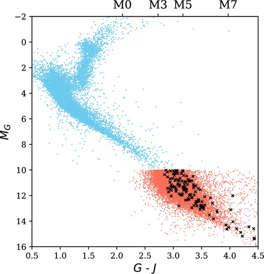
HR diagram of the stars targeted in this survey, shown in orange. Stars which flared are shown with black crosses. The blue points indicate stars with I < 16 observed in the standard NGTS operations. We have plotted G − J to include stars too faint to have an RP magnitude. Shown also are the spectral types for each G − J colour, calculated from the average magnitudes for M stars from Cifuentes et al. (2020). Not included in this figure are stars that were too faint to have a parallax measurement, or be included in Gaia DR2.
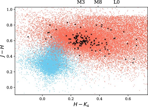
Colour–colour diagram for stars in our survey, using 2MASS J, H, and Ks magnitudes. The colours of points are the same as in Fig. 1.
2.2 Flare detection
For the faintest stars, a flare will result in the star becoming visible to NGTS for a short period of time. To detect flares in the NGTS light curves, we utilized the two-step detection method outlined in Jackman et al. (2021b), and used in previous searches for flares in NGTS light curves (Jackman et al. 2018, 2019a,b, 2020). We searched for flares from individual stars on a night-by-night basis. First, we searched for flare candidates within individual nights by flagging regions where there were at least three consecutive outliers lying six median absolute deviations (MADs) above the median of the nightly light curve. The MAD is a measure of the variance within a data set and is robust against the presence of outliers, such as those introduced by flare events, which will increase the standard deviation of a night. The second step of this method searches for flares that dominated the light curve of an entire night. An example of such a flare is the QPP-exhibiting flare discussed in Jackman et al. (2019a). To detect these flares for a given source, we compared the median of each night against the median of the entire light curve. A night was flagged in this step if its median lay five MAD above the median of the entire light curve. Both of these steps were performed through an automated method for each light curve in our data set, with flagged candidates saved to disc. Flagged candidates were then eyeballed to remove false positive candidates. Examples of false positive candidates include astrophysical signals due to variability other than flares (e.g. RR Lyrae), human-made signals due to satellites passing through apertures, and systematic trends.
Once we had eyeballed flare candidates to remove false positive signals, we checked each candidate to confirm the source of the flare. This was particularly important for sources with a nearby star contributing light to the photometric aperture. If the images are not checked, flares from a neighbouring flaring source can be mistakenly attributed to the target of interest. To verify our flare sources, we followed a similar method to Yang et al. (2017), Yang & Liu (2019), and Jackman, Shkolnik & Loyd (2021a), who searched for flares in the Kepler light curves. To isolate the flare emission for each source, we calculated a residual image, by subtracting the pre-flare NGTS image from the peak-flare NGTS image. The pre-flare image was chosen to be that immediately before the start of the flare, to best match the quiescent stellar emission. We then used this residual image to verify the source of each flare event. Sources, where the flare was coming from a neighbouring star, were flagged and masked from our analysis.
2.2.1 Understanding our detection efficiency
In order to combine information from both the flaring and non-flaring stars in our analysis, we must understand the efficiency of our detection method. This has added importance in this analysis, due to our sample combining flares from stars that are too faint to detect in quiescence and those that are. To characterize the efficiency of our flare detection method, we used flare injection and recovery tests. We did this following the method outlined in Jackman et al. (2021b), which itself was based on the injection and recovery tests discussed in Davenport et al. (2014) and Jackman et al. (2020). This method involves injecting flare templates of known duration, amplitude and energy into light curves, and measuring which flares are successfully identified with our chosen detection method. In this work, we used the empirical flare model from Davenport et al. (2014). This model was created from 1-min short cadence Kepler observations of flares from the active M dwarf GJ 1243 and is regularly used in the literature to model simple flare events (e.g. those lacking significant substructure). This model enables users to create flares using the amplitude and the t1/2 duration, or the full width at half-maximum (FWHM). We first used this model to generate a grid of artificial flares with t1/2 durations between 30 s and 70 min, and amplitudes up to 2000 times the quiescent flux of the star. We used the quiescent flux values from Section 2.4 for calculating the amplitude. We chose a maximum amplitude value of 2000 rather than a smaller value such as those used by previous studies (e.g. Günther et al. 2020; Jackman et al. 2021b) as we need our flare injection tests to probe our sensitivity to the highest energy flares. Along with this, for many of our stars, we will only be sensitive to flares with amplitudes of several magnitudes, necessitating the injection of very high-amplitude flares.
Once we had generated our grid of flares, we performed our flare injection. For each star, we injected 50 flares per night, drawing the amplitude and t1/2 duration of each flare randomly from our grid. We ran our flare detection algorithm on each night and recorded whether we would have detected each event, along with the energy of each injected event. We used this recorded data to calculate how the efficiency of our detection method changes as a function of energy for each star. Our detection efficiency should be zero for the lowest amplitude and energy flares (e.g. E < 1031 erg), whereas for the highest amplitude and energy events (e.g. E > 1034 erg) it should approach unity. For each star, we placed our injected flares into 20 bins spaced logarithmically in energy, and calculated the fraction of detected flares per bin. We then followed Davenport (2016) and used a smoothing Weiner filter, with a window size of three bins, to calculate our final detection efficiency for each star. We also calculated our detection efficiency as a function of amplitude, so we are able to calculate our flare incidence rates as functions of both energy and amplitude in Section 3.3.
2.3 Stellar characterization
We characterized the sources in each NGTS field by fitting their spectral energy distribution (SED). We did this using the BT-Settl grid of models (Allard, Homeier & Freytag 2012), which allowed us to go to effective temperatures below 2300 K. Where possible, we cross-matched each source in our target list with Gaia DR2, 2MASS, WISE (Cutri & et al. 2014) and Pan-STARRS (Chambers et al. 2016) to obtain astrometric information and broad-band photometry. Where possible we have obtained the distance to sources by cross-matching them with the catalogue of Bailer-Jones et al. (2018), which measures distances from Gaia DR2 parallaxes. We then followed the method of Gillen et al. (2017) and convolved each filter with the BT-Settl models, to create a grid of bandpass fluxes in Teff–log g space. To perform SED fitting for each star in our target list, we used least squares fitting. We chose this over an MCMC process, as has been used in previous flare studies, for the comparative speed of fitting all stars in our target lists. By fitting all stars, both flaring and non-flaring, we are able to probe the average flaring behaviour of ultracool dwarfs, rather than just the behaviour of individual flare stars. This is particularly important for our analysis of the flare incidence in Section 3.3. During this process, we fitted for the effective temperature Teff, surface gravity log g, and a scaling factor S. This scaling factor was used to renormalize the model photometry to match the observed values, and was equal to (R*/d)2, where (R*) is the stellar radius and d is the distance. To calculate the stellar radii, we multiplied the scale factor for each star by the corresponding Gaia DR2 distance value. For sources, which do not have a distance measured by Bailer-Jones et al. (2018), we used the values for the effective temperature and absolute J magnitude of M and L dwarfs from Cifuentes et al. (2020) to calculate the absolute J from our best-fitting SED temperature. We then used this absolute magnitude with the apparent 2MASS J magnitude to calculate the distance.
To account for extinction and reddening in each star, we first cross-matched each source with the 3D dust maps of Green et al. (2019). These maps combine Pan-STARRS and 2MASS photometry with Gaia astrometry to provide probabilistic estimates for reddening along a given line of sight. For stars that were covered by this map and have a Gaia DR2 distance, we used the median predicted value for the extinction AV at the listed distance. For stars without distances, we performed a preliminary SED fit to constrain Teff and S. These stars posed a unique problem, as by being too faint for Gaia distance values, they may either be very low-mass nearby M or L dwarfs (such as the flaring L2.5 dwarf discussed by Jackman et al. 2019b) where reddening can be ignored, or further away faint higher mass stars where reddening becomes more important. To try and account for this, we compared this preliminary Teff to the Baraffe et al. (2015) stellar models for main-sequence stars to estimate the radius and, in turn, the distance of our given star. This estimated distance was then used with the Green et al. (2019) dust maps to obtain a measure of the extinction and reddening, which was carried into our final SED fitting. Stars that were not covered by the Green et al. (2019) dust map were assumed to close by and assigned a value of AV = 0 with a standard deviation equal to the value from the Schlegel, Finkbeiner & Davis (1998) reddening maps (e.g. Green et al. 2021). We used our estimated values of AV as a fixed value in our SED fitting, using the extinction law of Fitzpatrick (1999) with the improvements applied by Indebetouw et al. (2005). When applying the effects of extinction and reddening to our fitted SEDs we used RV = 3.1.
2.4 Flare amplitudes
The amplitude of white-light flares is commonly calculated from the fractional flux F/Fq − 1, where F is the measured flux at the peak of the flare light curve and Fq is the quiescent stellar flux. To measure Fq studies will calculate the median flux of the quiescent light curve either around or immediately preceding a flare (e.g. Howard et al. 2019). However, as many of the stars in our survey are too faint to detect during quiescence, we cannot directly measure Fq in this manner. To measure the amplitudes of the flares detected in our survey from stars that are too faint for NGTS to measure a quiescent flux, we follow a method similar to that used by Jackman et al. (2019b) and calculate our flare amplitudes in terms of magnitude using
where mq and m are the quiescent magnitude and peak magnitude (during the flare), respectively. We obtained the quiescent magnitude mq for each flare star from our cross-matching with catalogue photometry in Section 2.3. To calculate a flare amplitude, we first measured the instrumental magnitude within the NGTS filter at the peak of the flare. We then converted this NGTS instrumental magnitude to the same bandpass as the quiescent magnitude by applying a linear relation between the two filters. This linear relation was measured by cross-matching all low-mass stars within each NGTS field with the chosen catalogue. We then used the converted NGTS magnitude with the catalogue quiescent magnitude with equation (1) to calculate the amplitude of each flare. We used three reference bandpasses when calculating flare amplitudes. These were, in ranked preference, the Gaia G, Pan-STARRS i′ and 2MASS J filters. If one was not available, we used the next best available catalogue magnitude. By using catalogue photometry to calculate the quiescent instrumental flux of each flare star, we have been able to account for the intrinsic faintness of many of our sources. For the stars that were bright enough for NGTS to detect in quiescence, we measured Fq directly by calculating the median of the light curve 10 min before the start of the flare. We also calculated the amplitudes of these flares using the method applied to the faint stars. We found agreement between the amplitudes measured by each method, and a comparison is shown in Fig. 3. To determine whether a star was bright enough to measure the quiescent flux directly, we compared its catalogue magnitude to an empirical limit measured from our cross-match between the instrumental and catalogue magnitudes. This limit was implemented because our sample includes stars that while too faint to be included in the standard NGTS analysis, were bright enough to detect in quiescence. We calculated the median and MAD of every NGTS light curve and flagged stars where the median was less than three times the MAD. We then obtained the corresponding catalogue magnitudes of each of these stars. We took the fifth percentile of these catalogue magnitudes as our empirical limit for when a star became too faint to directly measure the quiescent flux from the NGTS light curve. By combining these methods, we could calculate the flare amplitudes of both stars that were too faint and bright enough for NGTS to detect in quiescence.
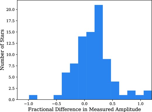
Histogram showing the fractional difference between the amplitudes measured using the methods for bright stars and for faint stars (depending whether or not they are detected by NGTS in quiescence).
2.5 Flare energies
We followed the method from Jackman et al. (2019b) to calculate the energy of each flare. We assumed that the flare spectrum can be modelled with a 9000 ± 500 K blackbody. This assumption is based on optical multicolour and spectroscopic observations of flares from active M stars (Hawley & Fisher 1992; Kowalski et al. 2013). The approximation of the flare spectrum as a 9000 K blackbody is commonly used in white-light flare studies to measure the bolometric energy of flares (e.g. Shibayama et al. 2013; Günther et al. 2020), allowing us to compare our results to previous works. However, we note here that recent studies have shown that the temperatures of white-light flares can vary both within and between events (e.g. Loyd et al. 2018; Froning et al. 2019; Howard et al. 2020a). This is especially relevant around the impulsive rise phase of flares, where these works have measured optical and FUV continuum temperatures of up to 40 000 K. However, while these results do limit the use of a single temperature flare model, we are currently not able to predict the temperatures of individual flares, limiting us from using a more detailed model that may incorporate flare feature-related temperature changes.
To calculate the flare energy, we used the flare amplitude light curve obtained in Section 2.4. We normalized the flare blackbody to match the stellar quiescent flux within the NGTS bandpass. For each time-step, in the flare light curve, we multiplied this renormalized blackbody by the corresponding flare amplitude, integrated it over all wavelengths and multiplied it by 4πd2 to calculate the flare luminosity. Here, d is the distance to the star, which we discussed in Section 2.3. This series of flare luminosities was then integrated over time to obtain the bolometric flare energy. We propagated the uncertainty of the stellar parameters and flare temperature to our final energy using a Monte Carlo method (e.g. Pugh et al. 2016; Jackman et al. 2021b). We generated 1000 blackbody curves with temperatures drawn from a normal distribution with a mean of 9000 K and standard deviation of 500 K (e.g. Hawley & Fisher 1992; Kretzschmar 2011; Pugh et al. 2016) We performed the above energy calculation with each of these 1000 blackbody curves and took the median result as our final energy, and used the 16th and 84th percentiles to measure the lower and upper uncertainties, respectively.
2.6 Flare duration
When measuring flare time-scales, we are limited by the fact that, depending on the stellar brightness, we may not be able to observe the flare for its full duration. Consequently, to provide relevant information about how long flares from ultracool dwarfs can last for, we have measured the duration of our flares using two methods. First for every flare, we have measured the ‘visible duration’, the length of time a flare is visible in NGTS. We measured this property directly through visual inspection of the NGTS light curves. For stars that are visible in quiescence, this is equal to the full flare duration as measured in previous flare studies (e.g. Jackman et al. 2021b).The other property we measure is the t1/2 time-scale, also known as the FWHM of the flares. This is the duration for which the flare is above half the maximum flux. To measure this we, use our flare amplitude light curves from Section 2.4. For flares from stars that are too faint to detect in quiescence, we only report this value for flares that are detected both above and below their half-flux level. For complex flares, we report the duration between the first and last time the flare goes above and below the half level (e.g. Loyd et al. 2018).
2.7 Flare impulse
Another metric we are able to calculate for the flares in our sample is the impulse. The flare impulse, |$\mathcal {I}$|, is defined as the ratio between the amplitude and t1/2 time-scale of the flare (Kowalski et al. 2013), and provides a metric for evaluating the evolution of the flare morphology around the peak. As the impulse depends on both the flare amplitude and the t1/2 time-scale, both a very short duration or a very high-amplitude flare will have a large impulse value. Previous studies have measured impulse values between 10−4 and 100 for flares from M dwarfs, using observations in different filters (Kowalski et al. 2013; Howard & MacGregor 2022), and used these values to describe the morphology of particular flares as gradual (|$\mathcal {I}\lt 1$|) or impulsive (|$\mathcal {I}\gt 1$|). We have used our measured amplitude and t1/2 values to calculate the impulse for each flare in our sample.
3 RESULTS
We have detected 160 flares from 135 stars from a search of 20 NGTS fields. These sources range from M3 to L2.5. We have provided the flare amplitudes and energies, and host star properties as a machine-readable table. The first five rows are shown as an example in Table 2.
Properties of the first five flares detected in our sample and their host stars. The full table is available as a machine-readable file online. The J flag indicates distances calculated from the absolute J magnitude–distance relation from Cifuentes et al. (2020).
| Field name | RA | Dec. | 2MASS | Distance (pc) | J Flag | Teff(K) | ΔmNGTS | E (erg) |
|---|---|---|---|---|---|---|---|---|
| NG0531–0826 | 05:28:02.73 | −07:54:38.48 | 05280272–0754382 | 161.42 ± 5.37 | N | |$2639^{+21}_{-22}$| | 1.56 | |$1.16^{+0.11}_{-0.10}\times 10^{34}$| |
| NG0531–0826 | 05:32:22.10 | −08:45:11.89 | 05322209–0845122 | 165.90 ± 9.51 | N | 3052 ± 22 | 2.99 | |$6.98^{+0.60}_{-0.63}\times 10^{34}$| |
| NG0531-0826 | 05:32:51.86 | −07:40:29.94 | 05325186–0740300 | 306.54 ± 17.38 | N | |$3172^{+25}_{-21}$| | 3.04 | |$3.19^{+0.27}_{-0.22}\times 10^{35}$| |
| NG0531–0826 | 05:33:01.25 | −09:04:36.16 | 05330125–0904362 | 625.35 ± 150.33 | N | |$3213^{+28}_{-31}$| | 2.50 | |$1.68^{+0.14}_{-0.13}\times 10^{35}$| |
| NG0531–0826 | 05:26:46.02 | −07:19:32.14 | 05264600–0719321 | 308.45 ± 25.52 | N | |$3127^{+51}_{-56}$| | 3.46 | |$6.04^{+0.65}_{-0.76}\times 10^{35}$| |
3.1 Flare energy
Where possible we calculated the bolometric energy of flares detected in our survey, following the method outlined in Section 2.5 and assuming the flare spectrum can be modelled with a 9000 K blackbody curve. The energies calculated range between 4.3 × 1031 and 1.1 × 1036 erg for spectral types M3 to L2.5. If we isolate those stars that were too faint to see in quiescence, the energies vary between 8.9 × 1031 and 6.0 × 1035 erg. If we focus specifically on ultracool dwarfs, our energies range between 4.3 × 1031 and 4.5 × 1034 erg, for eight flares.
As we are studying the highest amplitude flares, we have used our sample to study how the maximum flare energy varies with spectral type. This is shown in Fig. 4. This upper envelope has been studied previously using Kepler and NGTS by Davenport (2016) and Jackman et al. (2021b), respectively, to investigate whether there is an intrinsic maximum limit in the energy that can be released from flares. Jackman et al. (2021b) found that while they did identify an apparent upper limit in the flare energies of K and early-M stars observed with NGTS, this was consistent with not having observed for long enough to detect the rarest, highest energy, events. In addition to this, the observing strategies of these surveys also meant that studies of the maximum flare energies were limited to stars earlier than mid-M spectral type, as stars below this were typically too faint to be included in photometric target lists. We have been able to use our sample to study the maximum flare energies on stars later in spectral type than mid-M. We find that late-M stars in our sample broadly exhibit flares with energies up to 1035 erg, with a slight decrease in the observed maximum energies for ultracool dwarfs. To test whether we are probing the flare energy limit, we compared our results to those from Schmidt et al. (2019). Another study that has investigated the energies of large amplitude flares from late-M stars is Schmidt et al. (2019), who used ASAS-SN observations. Schmidt et al. (2019) used ASAS-SN observations to study the energies of high-amplitude flares from mid-to-late M stars. They found lower energy limits in the V band up to log (EV) = 34.5 erg, which using the V band to bolometric energy conversion from Rodríguez Martínez et al. (2020) correspond to EBol = 35.9 erg. This suggests that similar to the results for early M stars from Jackman et al. (2021b), the upper envelope of our sample in Fig. 4 is not the true limit of flare energies, and is instead due to the selection effect of our finite observing time not being enough to sample the highest energy events, which by their nature are also the rarest. Future studies with greater numbers of NGTS fields and data will aim to rectify this in the future, by sampling greater numbers of ultracool dwarfs.
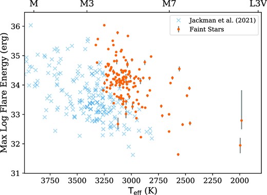
Maximum observed flare energy against effective temperature for M and L dwarfs in our sample. The orange circles indicate stars in our sample. The blue crosses are flare stars detected in the NGTS survey data from Jackman et al. (2021b). Our sample fills in the gap left by the I < 16 sample from Jackman et al. (2021b), showing that the apparent drop off in maximum flare energy for mid-M stars was a selection effect from low numbers of such stars in their sample. Errors were calculated using the method described in Section 2.5.
3.2 Flare amplitudes
We measured the amplitude of all flares in our survey, following the method outlined in Section 2.4. The amplitudes within the NGTS filter for our full sample ranged between ΔmNGTS = 0.3 and 6.2. If we filter our sample to stars that were too faint to see in quiescence, this range changes to between 1.7 and 6.2. We believe that the increased values of flare amplitude for the faintest stars is a selection effect, as we are unable to detect lower amplitude flares from these stars. If we filter on spectral type, we find that for mid-to-late M stars (M4–M7) stars, the flare amplitudes ranged between 0.3 and 5.7 for the full sample, and 1.7 and 5.3 for faint stars only. For ultracool dwarfs (M8 onwards), our measured amplitudes ranged between 1.0 and 6.2 for all stars, and 3.4 and 6.2 for faint stars. We believe that the increase in maximum flare amplitude for lower mass and temperature stars is due to the increased contrast between the flare spectrum and the quiescent photosphere within the NGTS filter. This means that a flare of fixed peak luminosity will have a larger amplitude for an M8 star than an M4 star. As shown in Fig. 4, the maximum flare energy is broadly constant for mid- to late-M stars, in turn, resulting in our observed increase in flare amplitudes.
3.3 Flare incidence
By including both the flaring and non-flaring stars in our analysis, we can study the fraction of low-mass field stars that exhibit flares in our sample. The wide range of quiescent magnitudes means that our detection method will not be sensitive to the same amplitude flares on all stars. For example, for the stars, we cannot detect in quiescence we will only be able to detect the highest amplitude flares. For stars that we can detect in quiescence, we will detect both these flares and lower amplitude ones. To account for the sensitivity of our detection method, we used the results of our flare injection and recovery tests from Section 2.2.1. For every star in our sample, we measured the flare amplitude corresponding to a 68 per cent detection efficiency. We then used our values to measure the flare incidence rate for amplitudes above chosen values. By requiring a 68 per cent detection efficiency, we ruled out stars for which we would not be able to detect a flare with at least a 1σ confidence in our detection efficiency.
To determine the fraction of mid-to-late M stars that showed high-amplitude white-light flares, we required that each star in our analysis had a Gaia DR2 distance from Bailer-Jones et al. (2018). This allowed us to rule out potential red giant interlopers from our 2MASS-colour sample, that would lower the measured fraction of flare stars. We note here that we do not have age information for our stars. However, our values will be representative of the average behaviour of field stars surveyed by future wide-field surveys such as the LSST. We calculated the uncertainties on the fraction of flares by assuming a binomial distribution (e.g. Howard et al. 2019). We calculated the fractions of flares with amplitudes above 1, 2, and 3 mag in the NGTS filter for M4–M6 and M7–M8 stars. These results are given in Table 3. We calculated these values by dividing the number of unique flaring stars by the total number of stars in each subset. We find that 1.4 ± 0.4 and |$9.1^{16}_{3.0}$| per cent of M4–M6 and M7–M8 stars, respectively, flare with amplitudes above 1 mag in the NGTS filter. We also find that higher amplitude flares, which broadly correspond to the rarer higher energy events, are rarer in both spectral bins. We also find that for a fixed amplitude, the incidence increases for the later spectral type M7–M8 bin. We attribute this to the increased contrast between the flare and quiescent spectrum in the NGTS filter for these stars, which means that lower energy (and more common) flares have amplitudes above 1 mag.
The percentage of mid-to-late M stars that showed high-amplitude flares in our analysis. These values were calculated using stars that had detection efficiencies of 68 per cent at each amplitude, as calculated through flare injection and recovery tests. The values in brackets note the total number of stars in the sample, and the number of stars which flared.
| ΔmNGTS = 1 | 2 | 3 | |
|---|---|---|---|
| M4–M6 | 1.4 ± 0.4 (771,11) | 0.48 ± 0.11 (3510,17) | 0.13 ± 0.03 (9673,13) |
| M7–M8 | |$9.1^{+16}_{-3.0}$| (11,1) | |$3.2^{+6.8}_{-1.2}$| (31,1) | |$1.1^{+2.9}_{-0.1}$| (89,1) |
| ΔmNGTS = 1 | 2 | 3 | |
|---|---|---|---|
| M4–M6 | 1.4 ± 0.4 (771,11) | 0.48 ± 0.11 (3510,17) | 0.13 ± 0.03 (9673,13) |
| M7–M8 | |$9.1^{+16}_{-3.0}$| (11,1) | |$3.2^{+6.8}_{-1.2}$| (31,1) | |$1.1^{+2.9}_{-0.1}$| (89,1) |
We also used our sample to study the fraction of flaring epochs (e.g. Kowalski et al. 2009; Chang, Wolf & Onken 2020), to measure how likely an M star will be flaring above a given amplitude at any instant. We calculated these by first calculating the total time stars in each sample were flaring with a flux above the amplitude limits specified in Table 3. We then divided these values by the total time each sample was observed for. This gives the instantaneous possibility of observing a flare with an amplitude above each limit. These values also provide a reference for transient surveys that may wish to predict the chance of observing a high-amplitude flare from an M dwarf at any one moment. These results are shown in Fig. 4. We find that in any given NGTS 13 s observation, there is a 6.5 ± 0.7 × 10⁻⁵ per cent chance a mid-M star is flaring with a flux one magnitude above its quiescent level. This value changes to 1.7 × 10 ± 0.3 × 10⁻³ per cent for late-M stars. We find that these values are much lower than the corresponding values in Table 3. This is due to the fact that most stars in our sample spend only a small fraction of their time flaring with the large amplitudes studied here.
The percentage of epochs that were flaring above a given amplitude value. As in Table 3, these values were calculated using stars that had detection efficiencies of 68 per cent at each amplitude, as calculated through flare injection and recovery tests.
| ΔmNGTS = 1 | 2 | 3 | |
|---|---|---|---|
| M4–M6 | 6.5 ± 0.7 × 10⁻⁵ | 5.6 ± 0.3 × 10⁻⁵ | 1.4 ± 0.1 × 10⁻⁵ |
| M7–M8 | 1.7 ± 0.3 × 10⁻³ | 1.7 ± 1.7 × 10⁻⁵ | 2.4 ± 1.2 × 10⁻⁵ |
| ΔmNGTS = 1 | 2 | 3 | |
|---|---|---|---|
| M4–M6 | 6.5 ± 0.7 × 10⁻⁵ | 5.6 ± 0.3 × 10⁻⁵ | 1.4 ± 0.1 × 10⁻⁵ |
| M7–M8 | 1.7 ± 0.3 × 10⁻³ | 1.7 ± 1.7 × 10⁻⁵ | 2.4 ± 1.2 × 10⁻⁵ |
3.4 Flare durations
As discussed in Section 2.6, we measured the duration of each flare we detected. We did this through multiple methods, which we will discuss the results of here. First, we calculated the t1/2 time-scale of every flare, the time the flare flux is above 50 per cent of the flare amplitude. We find that t1/2 values range between 23 s and 38 min or mid-M stars, and 30 s to 8.8 min for ultracool dwarfs. We have plotted the t1/2 duration against the measured energy for our flares in Figs 5 and 6. We find that there is overlap between flares from stars we could and could not detect in quiescence. This overlap is due to the t1/2 time-scale being a measure of the duration around the peak of the flare. We are able to observe this flare region from both faint and brighter stars. For the ultracool dwarfs in Fig. 6, the smaller sample limits our analysis. However, we find that faint stars can have flares with t1/2 durations between 1 and 2 min can have energies up to approximately 4 × 1033 erg. For both samples, we attribute the lack of flares at long t1/2 durations and low flare energies to the sensitivity of our detection method, as opposed to a lack of flares (e.g. Jackman et al. 2021b).
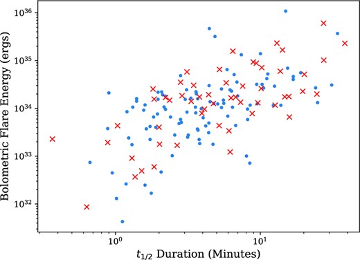
The bolometric energy against the t1/2 duration for flares from mid-M stars in our sample. The blue points and red crosses indicate stars that were and were not detected in quiescence, respectively.
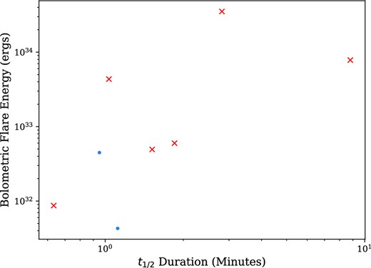
The bolometric energy against the t1/2 duration for flares from ultracool dwarfs in our sample.
For these stars, we have also measured the full visible duration, determined by eye. The values for our full sample range between 90 s and 1.84 h. If we filter our sample to the stars that were too faint to detect in quiescence, this range changes to between 90 s and 1.74 h.
3.5 Flare impulse
We measured the flare impulse of events in our sample, shown against effective temperature in Fig. 7. The impulse is the ratio between the flare amplitude and the t1/2 duration and provides a measure of how rapidly the flare light curve changes around the peak. We measured impulse values between 0.04 and 161. Our most impulsive flares came from the faint ultracool dwarfs in our sample, suggesting that these events are capable of releasing energy and evolving on very short time-scales. In addition to this, we found that all our flares from ultracool dwarfs have an impulse value |$\mathcal {I}$| greater than 1, making them impulsive flares (Kowalski et al. 2013). This is something we discuss further in Section 4.6.
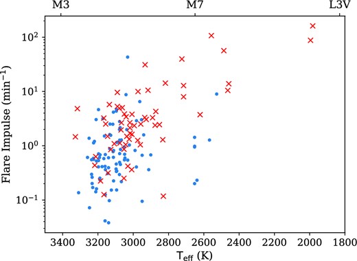
The flare impulse against effective temperature for stars in our sample. As in Fig. 5, the blue points and red crosses indicate stars that were and were not detected by NGTS in quiescence. We attribute the lack of flares in the bottom right-hand region due to the sensitivity of our detection method.
4 DISCUSSION
4.1 Flare amplitude and the impact of flare temperature
In Section 3.2, we presented the results of our flare amplitude measurements, finding that for stars between M4 and M7 the flare amplitudes ranged between 0.3 and 5.7 mag in the NGTS filter. For ultracool dwarfs, the flare amplitudes ranged between 1.0 and 6.2, highlighting how we are able to detect higher amplitude flares from cooler stars due to the increased contrast between the flare and quiescent spectrum. We are also able to use our results to estimate the g′ and U-band amplitude of flares in our sample, for comparison with surveys such as the Vera Rubin observatory (Ivezić et al. 2019) that will cover large fractions of the sky each night and detect rare high-amplitude flare events. If we assume the flare spectrum is given a 9000 K blackbody, then our measured amplitudes for mid -to-late M stars in the g′ and U bandpasses range between 1.3 and 8.2 mag and 3.4 and 11.0 mag, respectively. For ultracool dwarfs, these change to 4.4 and 11.1 for g′ and 7.8 and 16.4 for U band.
However, recent studies have found evidence for flare temperatures beyond 9000 K at the peaks of flares (e.g. Kowalski et al. 2013; Loyd et al. 2018), in some cases reaching up to 40 000 K for high-energy flares from low-mass stars (e.g. Froning et al. 2019; Howard et al. 2020b). Along with this, Howard et al. (2020b) found evidence for an increase in the peak flare temperature with flare energy in low-mass stars. As we are probing the highest energy events from ultracool dwarfs, it is possible that the flares in our sample have temperatures greater than 9000 K. Such temperatures would increase the flare amplitude in filters bluer than NGTS. We therefore also calculated the range of flare amplitudes assuming a peak flare temperature of 40 000 K and the same amount of flux in the NGTS bandpass. In this scenario, we expect flare amplitudes up to 8.8 and 12.4 mag in the g′ and U bands for M4–M7 stars, and up to 11.8 and 17.7 mag for ultracool dwarfs. We note that these values should be taken as examples of the maximum possible amplitudes in these filters for flares in our sample, as only a few flares observed spectroscopically or with two-colour photometry have had measured temperatures reaching 40 000 K. Regardless of this, these values highlight the explosive nature of these events, and the flares that could be detected with NGTS.
4.2 Flare incidence in surveys
In Section 3.3, we measured the fraction of mid-to-late M dwarfs in our sample that showed high-amplitude flares. We found that 1.4 ± 0.4 per cent of M4–M6 stars exhibited flares with an amplitude above 1 mag in the NGTS filter. We also found that the incidence rate of flares decreased with amplitude, namely that higher amplitude flares were rarer than lower amplitude ones. Flares are known to occur with a power-law distribution in both energy and amplitude, so this result is not unexpected (e.g. Howard et al. 2019). We found that for a given amplitude, the flare incidence increases as we go to lower mass M7–M8 stars. We believe this is due to the changing contrast between the flare and quiescent spectrum, as discussed in Section 3.2. As we go to lower mass and temperature stars, the contrast between the blue flare spectrum and the quiescent stellar spectrum increases. Therefore, flares of the same energy will appear larger on lower mass stars. Consequently, as we got to later spectral types, events within a fixed amplitude bin will correspond to lower energy flares. As mentioned above, flares are known to occur with a power-law distribution in energy (e.g. Lacy et al. 1976; Gershberg & Shakhovskaia 1983; Hawley et al. 2014), with lower energy flares occurring more often than higher energy ones. Therefore, we are probing more common flares and the incidence of detected flares increases, as observed.
We note that other studies that have measured higher flare incidence rates for mid-M stars than those we have presented in Table 3. For example, Rodríguez Martínez et al. (2020) used ASASSN V-band photometry to measure a flare incidence rate of ∼ 25 per cent for M5 stars, while Howard et al. (2019) used EvryScope g′ data to measure a rate of ∼20 per cent for M4 stars. In redder bandpasses, Yang & Liu (2019) measured a flare rate for early- and mid-M stars of 9.74 per cent from Kepler observations, while Günther et al. (2020) measured a rate of 30 per cent for M4–M6 stars with TESS 2-min cadence observations. Murray et al. (2022) measured fractions of 30–60 per cent for M4–M8 stars observed with SPECULOOS, values that are much higher than those presented in Table 3. We believe the increased flare rates measured by these studies can be attributed primarily to the amplitude limits we have imposed in Table 3. As discussed above, flares have been shown to occur with a power-law distribution in amplitude and energy, with higher amplitude and energy flares being rarer than their smaller counterparts. Previous studies with higher measured flare rates have typically not imposed a magnitude limit on the incidence. Therefore their samples include more common low amplitude events, increasing the measured fraction of flaring stars. Studies using Kepler and TESS data probe a similar region of the flare spectrum as the NGTS bandpass, however, focus on stars that can always be detected in quiescence, allowing them to detect much lower amplitude flare events. This is also the case for the SPECULOOS data presented by Murray et al. (2022). These observations used a I + z′ filter that covers a similar wavelength range as the NGTS filter, and Murray et al. (2022) was able to detect flares down to an amplitude of 1 per cent in the SPECULOOS light curves. This amplitude threshold is much lower than the one enforced here (approximately 150 per cent), resulting in a higher rate of detections from lower amplitude events.
Other studies that make use of bluer photometry will also benefit from flares appearing larger in their observations than they would in equivalent NGTS photometry. For example, as discussed in Section 2.4, if we assume a 9000 K blackbody for the flare spectrum, a flare on an M5 star with an amplitude of ΔmNGTS = 1 will have g′ and V-band amplitudes of 2.8 and 2.4 mag, respectively. These values are above 98 and 100 per cent of the amplitudes measured in the Howard et al. (2019) and Rodríguez Martínez et al. (2020) samples with Evryscope and ASASSN, respectively. This increase in the measured amplitude once again allows these studies to detect lower energy flares that occur more often, resulting in higher flare incidence rates than those measured here.
We also presented incidence rates in terms of the fraction of flaring epochs in our observations. The rates for mid-M stars are shown in Table 4. We found that mid- and late-M stars flared 6.5 ± 0.7 × 10⁻⁵ and 1.7 ± 0.3 × 10⁻³ per cent of the time. We found that these values were lower than the corresponding values in Table 3, due to stars only spending a small fraction of their time flaring, while our values in Table 3 only required a star to flare once to be included in our flare sample. Our value for fluxes above one magnitude from M4–M6 stars are orders of magnitude lower than the epoch fractions measured by Kowalski et al. (2009) and Chang et al. (2020), but are more similar to those reported from the Palomar Transient Factory Sky2Night Programme by van Roestel et al. (2019). We again attribute this to our focus on higher amplitude flares and the use of bluer filters by other studies. This latter point was also noted by van Roestel et al. (2019), whose flare observations were in the R band and all had measured amplitudes above 0.6 mag. This result notes the importance of specifying amplitude limits when calculating flare incidence rates, along with the dependence of incidence rates on the chosen photometric filter.
4.3 Flare energies of ultracool dwarfs
In Section 3.1, we presented the calculated bolometric energies for flares in our sample. These bolometric energies assume the flare emission can be modelled with a 9000-K blackbody spectrum. We also presented how the maximum observed flare energies in our sample changed with spectral type. We found that the maximum energy continued from the observed behaviour for early-M stars from Jackman et al. (2021b), with most stars having maximum observed energies below 1035 erg. However, we noted that detections of flares with energies above these from other surveys (e.g. Schmidt et al. 2019) meant that upper envelope seen in Fig. 4 does not represent a true maximum energy limit for flares. While these may not represent the upper limit of flare energies, our detections are still some of the most energetic for flares from ultracool dwarfs.
We also note the detection of flares from two L dwarfs in Fig. 4. One of these is the L2.5 dwarf ULAS J224940.13–011236.9 reported by Jackman et al. (2019b). The other is from 2MASS J16331457+0118507. Our SED fitting gives a best-fitting effective temperature of |$1995^{+173}_{-180}$| K, resulting in a spectral type of L1.5 (Cifuentes et al. 2020). While still rare compared to M dwarfs, observations of flares from early L dwarfs have become more common in recent years. This is due to a combination of serendipitous discoveries and concerted efforts to obtain photometry of these ultracool objects (Schmidt et al. 2016; Gizis et al. 2017; Paudel et al. 2018; Jackman et al. 2019b; Paudel et al. 2020). The most recent of these studies, Paudel et al. (2020), used K2 photometry to obtain light curves of 45 L dwarfs, finding 11 flares on 9 of them. Eight of these were from early L dwarfs, giving a total number of 14 L0-L5 dwarfs with white-light flares. Our detection of a flare from 2MASS J16331457+0118507 brings this number up to 15. This star flared with an energy of |$8.9^{+6.4}_{-4.2}\times 10^{31}$| erg, placing it at the lower end of white-light flare energies detected from L dwarfs (e.g. Paudel et al. 2020). Our sample has no overlap with the Paudel et al. (2018, 2020) samples. We expect that with further study of the NGTS FFIs, we will be able to detect more flares from L dwarfs.
4.4 What is the impact of big flares from small stars?
The detection of terrestrial planets in the habitable zones around cool and ultracool dwarfs has meant that these systems have become a focus for studies of exoplanet habitability (e.g. Anglada-Escudé et al. 2016; Gillon et al. 2017; Gilbert et al. 2020). Their low temperatures mean that the habitable zone is closer in that for Solar-type stars. Therefore, the effects of flares on such planets will be exaggerated due to their close proximity to the host star. These effects include changes to the atmospheric chemistry and also providing potentially damaging levels of UV irradiation to surface-dwelling organisms (e.g. Abrevaya et al. 2020). To quantify the effects of the flares shown in Fig. 4, on a hypothetical Earth-like planet that resides in the habitable zone of each flare star, we calculated the ‘equivalent Carrington event’ of each flare. The equivalent Carrington event is a value designed to express the energy received at the top of the atmosphere of each hypothetical planet in units of the energy received by Earth during the 1032 erg flare from 1859 Carrington (1859) and Tsurutani et al. (2003). To calculate the habitable zone of each flare star, we have used the ‘moist greenhouse’ model from Kopparapu et al. (2013). As the relations from Kopparapu et al. (2013) are only applicable for stars with effective temperatures above 2600 K, we have only performed this work for our subset of mid-M stars. Our results are shown in Fig. 8. We can see that for the most energetic flares in our sample, the energy received at the top of the atmospheres is equivalent to over 100 000 times the energy received by Earth during Carrington event. We note that for 1033 erg flares from mid-M stars, events that are often observed in flare studies (e.g. Günther et al. 2020; Seli et al. 2021) and are 10 times more energetic than the Carrington event (Tsurutani et al. 2003), the close in nature of the habitable zone means that Earth-sized planets will still receive flux of approximately 1000 equivalent Carrington events. However, we will note here that we have assumed that each flare region is located on the stellar equator, meaning the planet will receive the maximum amount of flux. Studies have suggested that M dwarfs may exhibit starspots at higher latitudes than on the Sun, and possibly just within single hemispheres (e.g. Brown et al. 2020), resulting in flare regions at higher latitudes. Ilin et al. (2021a) recently used TESS short cadence observations of four rapidly rotating ultracool dwarfs to measure the latitude of the flare emission. They measured latitudes between 55° and 81°, higher than that seen on the Sun, suggesting that, at least for rapidly rotating ultracool dwarfs, flare emission comes from closer to the poles than the equator. Ilin et al. (2021a) also estimated the effect this would have on the flux received by an orbiting planet, finding that a flare at 81° had its flux attenuated by up to 85 per cent. While this would result in nearby planets receiving less flux at the surface, we note that each flare would still result in a nearby Earth-sized planet receiving an energy equivalent to over 100 Carrington events. This highlights the importance of the close proximity of these planets to their host stars, and how this can exaggerate the effects of flares.
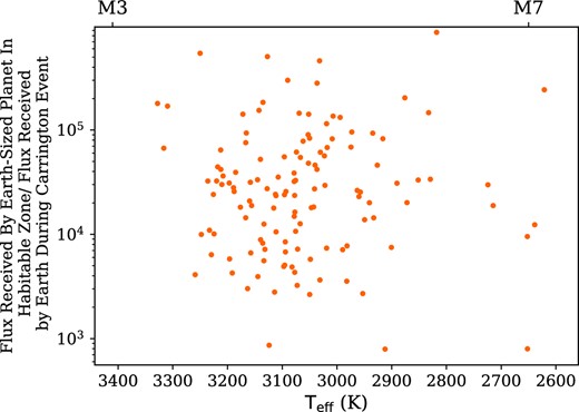
Flares from Fig. 4 plotted in terms of equivalent Carrington events. This is ratio between the flux received at Earth during the 1032 erg flare of 1859 (Carrington 1859; Tsurutani et al. 2003), and the flux received at the top of the atmosphere of a hypothetical Earth-sized planet in the habitable zone of each star. We calculated the location of the habitable zone for each star using the moist greenhouse model from Kopparapu et al. (2013). Note the highest energy flares are equivalent to the bolometric energy from over 100 000 Carrington events, due to the proximity of the habitable zone.
4.5 Flare duration and detecting similar events with TESS
In Section 3.4, we presented the measured durations for flares in our sample. We measured the durations in two ways, the t1/2 and total duration. We presented the distribution of t1/2 durations and bolometric flare energies for our mid-M and ultracool dwarfs in our sample in Figs 5 and 6. We found that for mid-M stars, flares with t1/2 durations above 10 min can have energies up to 1036 erg. We also note a lack of flares at long durations and low energies, which we attributed in Section 3.4 to the decreasing sensitivity of our detection method. To test this, we used the results of our flare injection and recovery tests. We found that, similar to Jackman et al. (2021b), the efficiency of our detection method drops off for lower energy and longer duration flares. This is likely due to the lower amplitude of these events, which in turn do not reach the thresholds for flare detection outlined in Section 2.2.
We found that the total durations of our flares ranged between 90 s and 4.6 h. When we considered only the flares from stars that were too faint to detect in quiescence, this range changed to between 90 s and 1.74 h. We are able to use our measured total durations to estimate whether other surveys may be able to detect similar flares from faint stars. In particular, we have investigated this for TESS, specifically for the TESS FFIs. As discussed in Section 1, previous studies have used TESS short cadence observations to study flaring activity of low-mass stars. However, these postage stamps are typically not placed on stars that are too faint to be detected in quiescence, such as ultracool M and L dwarfs. Consequently, the FFIs become the only option to detect flares from these faint stars. However, in the primary (Cycles 1 and 2) and first extended mission (Cycles 3 and 4) of TESS, the cadence of these images (30 and 10 min, respectively) may be too long to detect such events, that are only visible for short durations of time. However, in the second extended mission (Cycles 5 and 6), the FFI cadence changed to 200 s, meaning more flares are likely to be visible. For stars fainter than i′ = 13, NGTS, and TESS have comparable noise properties (Ricker et al. 2014; Wheatley et al. 2018). Consequently, we can use our results to inform what fraction of flares from faint stars can be detected in the publicly available TESS FFIs from the primary and first two extended missions.
To determine whether a flare in our sample would have been detected in each respective cadence mode, we require the full duration to be at least three times the TESS cadence. This is to better reflect the detection methods used in previous flare studies that require the detection of multiple data points above a set threshold before a signal is considered a flare candidate (e.g. Doyle, Ramsay & Doyle 2020; Tu et al. 2020; Jackman et al. 2021b). However, we note here that we have not incorporated the smearing effects of longer cadence observations that can reduce measured flare amplitudes, potentially resulting in some flares not reaching the thresholds required for a detection trigger (e.g. Yang et al. 2018; Howard & MacGregor 2022). We also note that despite the similar overall wavelength coverage, the NGTS bandpass has a shorter effective wavelength (6568 Å) than the TESS bandpass (7452 Å). Flares detected with NGTS would likely have smaller amplitudes in TESS light curves. These factors mean that our estimates of the flare incidence in TESS observations will be upper limits.
We find that for our full sample of flares from stars that are too faint to detect in quiescence, up to |$1.7^{+3.4}_{-0.7}$| per cent would have been detected in the 30-min cadence FFIs. This increases to |$22^{+6.6}_{-4.5}$| and |$87^{+5.9}_{-3.2}$| per cent for the 10- and 200-s cadence modes, respectively. As expected, the shorter cadence FFIs would have detected a greater fraction of flares. If we focus on our sample of flares from ultracool dwarfs, we find that both the TESS 30- and 10-min cadence FFIs would have detected up to |$17^{+24}_{-6.5}$| per cent, while the 200-s cadence FFIs would have detected up to |$67^{+13}_{-21}$| per cent of the flares in our sample. We note that the uncertainties here are larger than for the full sample due to smaller number of flares detected from ultracool dwarfs. However, it still shows that the 200-s cadence FFIs available in the TESS second extended mission should provide an excellent resource and opportunity for detecting the highest energy flares from the faintest M and L stars.
4.6 Flare impulse
In Section 3.5, we measured the impulse of each of the flares in our sample. The impulse is the ratio of the flare amplitude and t1/2 time-scale, and describes how quickly the flare light curve evolves around its peak. For our full sample we measured impulse values between 0.04 and 161, with the most impulsive flares coming from the faint ultracool dwarfs in our sample. Previous studies have measured impulse values (in units of min−1) between 10−4 and 100 (e.g. Kowalski et al. 2013; Howard & MacGregor 2022). We note that the impulse is dependent on the chosen bandpass, as bluer wavelengths can result in an increased amplitude and impulse. For reference, Howard & MacGregor (2022) used 20 s cadence TESS photometry of flares from M stars to measure impulse values between 10−4 and 4, while Kowalski et al. (2013) used U-band photometry to measure values between 0.02 and 96.0 for flares from active M stars. Our values for late M and L dwarfs reach up to and exceed these values, even though the NGTS bandpass covers similar wavelengths as TESS. This means that the high-energy flares we have detected from these stars are very impulsive, depositing the majority of their energy over short time-scales. Kowalski et al. (2013) measured the impulsiveness time-scale in the U band and the Balmer jump ratio of 20 flares from mid-M dwarfs and found that the most impulsive flares exhibit reduced Balmer jumps at their flare peaks. The Balmer jumps for the most impulsive events increased the continuum emission in the NUV by a factor of 1.5–2, whereas it was increased by factors of 3–4 for gradual events (Kowalski et al. 2019). The peaks of impulsive flare events were noted by Kowalski et al. (2013) as therefore having a stronger relative contribution from the thermal blackbody continuum. In total, 49 per cent of the flares in our sample have an impulse value greater than 1, while all of our flares from ultracool dwarfs in our sample have an impulse greater than 1. If the trend observed by Kowalski et al. (2013) holds for later spectral types, then we would expect the NUV continuum emission of high-energy flares from ultracool dwarfs to be slightly dominated by the thermal blackbody and not the Balmer continuum as for more gradual events.
However, we note that for faint stars, our detection method is biased towards more impulsive events. We confirmed this by using the results of our injection and recovery tests to calculate the impulse corresponding to the 68th perecentile of the detection efficiency for each ultracool dwarf in our sample. We find that we would not expect to detect any flares from ultracool dwarfs with impulses below values between 1 and 5. Consequently, the bottom right-hand region in Fig. 7 is a selection effect and ultracool dwarfs may still exhibit gradual flare events. However, the ones we do detect in our survey would suggest that some of the most impulsive, and perhaps thermal blackbody dominated, flare events may come from ultracool dwarfs.
5 CONCLUSIONS
We have presented the results of a targeted search for mid-M and ultracool stars with the NGTS. We used FFIs from 20 NGTS survey fields to target stars that we could detect in quiescence and stars that only became visible to us during a flare. We calculated the amplitudes, durations and, where possible, the energies of each detected flare. We detected 160 flares from 135 sources, which had spectral types ranging from M3 to L2.5. We calculated flare energies ranging between 4.3 × 1031 and 1.1 × 1036 erg. Of these flares, eight were from ultracool dwarfs, and had energies ranging between 4 × 1031 and 4.5 × 1034 erg.
We used our sample of stars to calculate the incidence rate of high-amplitude flares from mid-M stars. We found that 1.4 ± 0.4 and |$9.1^{+16}_{-3.0}$| per cent of M4–M6 and M7–M8 stars, respectively, flared with an amplitude above 1 mag in the NGTS filter. This value is lower than the flare incidence rates for mid-M stars reported by some other previous flare surveys, which we attribute to our focus on high-amplitude flares.
We used our measurements of the total visible durations to estimate the fraction of flares in our sample that would have been detected in different TESS observing modes. We found that for stars that were too faint to detect in quiescence, only |$1.7^{+3.4}_{-0.7}$| per cent would have been detected in the 30-min FFIs. However, this increased to |$22^{+6.5}_{-4.5}$| and |$87^{+5.9}_{-3.2}$| per cent of flares for the 10 min and proposed 200 s FFIs, respectively, highlighting the benefit of fast cadence observations in detecting high-energy flares from faint stars.
We intend to expand upon this work in the future to probe a larger sample of ultracool dwarfs. By incorporating more NGTS fields into our analysis, we will be able to increase the precision in spectral type for our analysis of the flare incidence rates and better probe the occurrence rates of the highest energy flares, allowing us to study the behaviour of the most extreme flare events.
Acknowledgement
This research is based on data collected under the NGTS project at the ESO La Silla Paranal Observatory. The NGTS facility is funded by a consortium of institutes consisting of the University of Warwick, the University of Leicester, Queen’s University Belfast, the University of Geneva, the Deutsches Zentrum für Luft- und Raumfahrt e.V. (DLR; under the ‘Großinvestition GI-NGTS’), the University of Cambridge, together with the UK Science and Technology Facilities Council (STFC; project references ST/M001962/1 and ST/S002642/1). JAGJ was supported by STFC PhD studentship 1763096 for this work. PJW, RGW, and SG acknowledge support by STFC under consolidated grants ST/P000495/1 and ST/T000406/1. JSJ acknowledges support by Fondecyt grant 1201371 and by the ANID BASAL project FB210003. This research has made use of the SVO Filter Profile Service (http://svo2.cab.inta-csic.es/theory/fps/) supported from the Spanish MINECO through grant AYA2017-84089.
DATA AVAILABILITY
Flare properties are provided as a supplementary file online.
