


ABSTRACT
We present an algorithm to extend subhalo merger trees in a low-resolution dark-matter-only simulation by conditionally matching them to those in a high-resolution simulation. The algorithm is general and can be applied to simulation data with different resolutions using different target variables. We instantiate the algorithm by a case in which trees from ELUCID, a constrained simulation of |$(500\, h^{-1}\, {\rm Mpc})^3$| volume of the local universe, are extended by matching trees from TNGDark, a simulation with much higher resolution. Our tests show that the extended trees are statistically equivalent to the high-resolution trees in the joint distribution of subhalo quantities and in important summary statistics relevant to modelling galaxy formation and evolution in halos. The extended trees preserve certain information of individual systems in the target simulation, including properties of resolved satellite subhalos, and shapes and orientations of their host halos. With the extension, subhalo merger trees in a cosmological scale simulation are extrapolated to a mass resolution comparable to that in a higher resolution simulation carried out in a smaller volume, which can be used as the input for (sub)halo-based models of galaxy formation. The source code of the algorithm, and halo merger trees extended to a mass resolution of |$\sim 2 \times 10^8 \, h^{-1}\, {\rm M_\odot}$| in the entire ELUCID simulation, are available.
1 INTRODUCTION
In the concordant Lambda cold dark matter (ΛCDM) cosmology, the peaks of the density field, known as dark matter halos, are the building blocks of large-scale structures of the Universe. Galaxies form and evolve through gas cooling and condensation in the gravitational background provided by dark matter halos (e.g. White & Rees 1978; Mo, van den Bosch & White 2010). Galaxies are complex ecosystems where various components, such as dark matter, gas, stars, and black holes, interact through complicated physical processes, presenting interesting and yet challenging problems for modern astrophysics. Enormous efforts, motivated by both theory and observation, have been made to model galaxy formation under various assumptions. Perhaps the most powerful approach to study galaxy formation is hydrodynamic simulation, which relies on the advances in computational resources and aims at modelling galaxies from first principles (e.g. Springel & Hernquist 2003; Springel 2010; Genel et al. 2014; Vogelsberger et al. 2014, 2020; Crain et al. 2015; Schaye et al. 2015; Marinacci et al. 2018; Naiman et al. 2018; Nelson et al. 2018, 2019; Springel et al. 2018; Pillepich et al. 2018b, 2019; Davé et al. 2019 ). Here physical processes for galaxy formation are simulated with a set of differential equations, complemented with subgrid physics to deal with situations of limited numerical resolution and uncertain processes on small scales. With careful calibrations, hydrodynamic simulations can successfully reproduce many statistical properties of the galaxy population and provide insights into physical processes underlying observational data.
To overcome some of the limitations of numerical simulations, particularly in computational costs and numerical uncertainties, a different category of methods, known as halo-based semi-analytical or empirical methods, have been proposed. These methods simplify the modelling of galaxy formation by splitting it into abstract layers that are assumed to be independent. Specifically, these methods use dark-matter-only (DMO) simulations (e.g. Springel 2005; Boylan-Kolchin et al. 2009; Feng et al. 2016; Habib et al. 2016; Wang et al. 2016, 2018; Falck et al. 2021; Frontiere et al. 2021) as input, find (sub)halos using some algorithms (structure/halo finders), link (sub)halos in different snapshots through some tree builders, and populate (sub)halos or trees with galaxies using empirical relations motivated by physical and observational priors. With such an abstraction, problems in each layer can be solved independently, so that the complexity in modelling the full process of galaxy formation is reduced. There is a vast literature in each of the steps. Examples of the structure finders include those based on the overdensity set obtained with boundary growing and pruning (Springel et al. 2005; Boylan-Kolchin et al. 2009; Planelles & Quilis 2010; Vallés-Pérez, Planelles & Quilis 2022), and those based on direct link of particles (Davis et al. 1985; Diemand, Kuhlen & Madau 2006; Behroozi, Wechsler & Wu 2012). Examples of tree builders include Monte Carlo methods based on the extended Press–Schechter (EPS) formalism (Somerville & Kolatt 1999; Cole et al. 2000; Parkinson, Cole & Helly 2007; Somerville et al. 2008; Zhang, Ma & Fakhouri 2008, see also Jiang & van den Bosch 2014 for a review), those based on linking simulated (sub)halos (Springel et al. 2005; Boylan-Kolchin et al. 2009; Han et al. 2012; Behroozi et al. 2013; Jiang et al. 2014), and those based on post-processing and homogenizing trees produced by other methods (Helly et al. 2003; Jiang et al. 2014). Examples of halo-based models include those matching galaxies and halos based on abundance (Mo, Mao & White 1999; Vale & Ostriker 2004; Guo et al. 2010; Simha et al. 2012), clustering (Guo et al. 2016) and age (Hearin & Watson 2013; Hearin et al. 2014; Meng et al. 2020; Wang et al. 2023), halo occupation distributions (HODs; Jing, Mo & Börner 1998; Berlind & Weinberg 2002; Guo et al. 2015, 2016; Qin et al. 2022; Yuan et al. 2022), the conditional luminosity function (CLFs; Yang, Mo & van den Bosch 2003; Zandivarez, Martínez & Merchán 2006; Yang, Mo & van den Bosch 2008; Robotham, Phillipps & De Propris 2010; Zandivarez & Martínez 2011; Meng et al. 2023) and conditional colour–magnitude distribution (CCMD; Xu et al. 2018), empirical models based on star formation histories of galaxies (Mutch, Croton & Poole 2013; Lu et al. 2014a, 2015b; Moster, Naab & White 2018; Behroozi et al. 2019; Moster et al. 2020), and semi-analytical models (SAMs) that emphasize more on physical motivated prescriptions than empirical models (White & Frenk 1991; Kauffmann, White & Guiderdoni 1993; Cole et al. 1994; Somerville & Primack 1999; Cole et al. 2000; Kang et al. 2005; Springel et al. 2005; Somerville et al. 2008, 2012, 2021; Guo et al. 2011; Ade et al. 2014; Popping, Somerville & Trager 2014; Lu et al. 2014b; Henriques et al. 2015; Lacey et al. 2016; Stevens, Croton & Mutch 2016; Baugh et al. 2019; Yung et al. 2019, 2023; Henriques et al. 2020).
The halo-based models described above capitalize heavily on structures resolved by DMO simulations. Because of computational limitations, these simulations always need to trade off between large simulation volumes and high numerical resolutions, because large volumes are needed to suppress cosmic variances (e.g. Somerville et al. 2004; Moster et al. 2011; Chen et al. 2019), while high resolutions are required to follow galaxy formation and evolution in halos/subhalos accurately. In particular, the properties of subhalos may not be properly resolved at high |$z$| when their masses are below the resolution limit of a large-box simulation. The limited resolution also makes the treatment of the evolution of satellite subhalos uncertain, as they may artificially lose particles and get destroyed as a result (e.g. van den Bosch et al. 2018; van den Bosch & Ogiya 2018; Green, van den Bosch & Jiang 2021). Thus, the application of a halo-based model to a cosmological-scale DMO simulation cannot rely solely on the assembly histories of subhalos provided by the simulation. Because of this, various methods have been adopted to extend the subhalo population in large-box simulations so as to trace the progenitors and subhalos that are missed. For example, Chen et al. (2019) used Monte Carlo trees generated from the EPS formalism to extend simulated trees in ELUCID. Yung et al. (2022, 2023) used EPS-based trees to replace the full assembly histories of halos in their adopted simulations. Chen et al. (2021) adopted the assembly histories of halos from a high-resolution DMO simulation to amend halo histories in a low-resolution DMO simulation, and found that this method is more accurate than the EPS-based amendment.
Some efforts have been made to use satellite subhalos in simulations to model satellite galaxies, but many of them rely on simple assumptions. For example, Chen et al. (2019) and Yung et al. (2022, 2023) did not use any information carried by satellite subhalos in simulations. Instead, they adopted a dynamic friction model to predict the lifetimes of satellite subhalos/galaxies, and used the Navarro–Frenk–White (NFW; Navarro, Frenk & White 1997) profiles of the host halos to assign phase-space coordinates (positions and velocities) to satellites. Because the assignment of phase-space coordinates is random and based on host halos in the current snapshot, the correlation of phase-space coordinates with other current and historical (sub)halo properties is lost. Consequently, the spatial distribution obtained this way may be biased for galaxies selected according to properties that are correlated to the history and environment of subhalos. Guo et al. (2015, 2016), Yuan, Eisenstein & Leauthaud (2020), Yuan, Hadzhiyska & Abel (2023), and Yuan et al. (2022) assigned galaxies obtained from HOD models to random particles in simulated halos. As tested by Bose et al. (2019) with a hydrodynamic simulation, radial distributions of satellite galaxies of given stellar mass match accurately the best-fitting NFW profiles of their host halos, which provides supports to the particle-based assignment scheme. However, the correlation between phase-space properties and other (sub)halo properties are still lost in this scheme. Li et al. (2021) and Ni et al. (2021) extended low-resolution DMO simulations by populating more particles in the simulation volumes, using deep-learning models trained by high-resolution simulations. This method preserves environmental information of the low-resolution simulation, but again, the extension is made at separate snapshots and thus loses information about subhalo formation histories. The two SAMs of GALFORM (Cole et al. 2000; Lacey et al. 2016; Baugh et al. 2019) and L-Galaxies (Henriques et al. 2015, 2020) used simulated phase-space information of satellite subhalos before they are disrupted, and linked a modelled ‘orphan’ galaxy, whose subhalo has been artificially disrupted, to the most bound particle of its subhalo just before disruption. This choice preserves some of the correlations of subhalos described above, but may introduce some other problems. For example, the most bound particles may be biased tracers of their subhalos after disruption, and a single particle in a shallow potential may accidentally lose its binding energy and jump to an unrelated location owing to numerical effects. Perhaps the ultimate solution to reliably resolving satellite subhalos is to use zoom-in simulations of individual subregions of interest (e.g. Kang et al. 2005; Barnes et al. 2017; Nelson et al. 2019). However, such high-resolution zoom-in simulations are still computationally expensive and thus infeasible to cover the volume of a large cosmological simulation.
To build a solid foundation for halo-based models, we develop in this paper a powerful algorithm to extend the resolution of subhalo merger trees in a low-resolution DMO simulation by conditionally matching them with those in another high-resolution DMO simulation. The extended trees have more complete assembly histories for low-mass halos at high-|$z$|, and satellite subhalos extend their lifetimes with assigned phase-space coordinates after they are disrupted by numerical effects. As we will show, the extension algorithm not only reproduces the joint distribution of various subhalo properties, including their phase-space coordinates, but also tries to maximally keep information about individual systems resolved by the target low-resolution simulation, such as properties of satellite subhalos and shapes of their host halos. With such an extension, halo-based galaxy formation models can be built on more complete (sub)halo assembly histories and more reliable predictions for the galaxy population.
This paper is organized as follows. In Section 2, we introduce the simulation data used in our analysis. In Section 3, we describe the algorithm to extend subhalo merger trees. We first present a general scheme that is applicable to a wide range of input data, and then specify cases studied in the present paper. In Section 4, we present tests on the performance of the extension on various properties of the merger trees and the subhalo population. Finally, we summary and discuss our main results in Section 5. Code and data availability are described in the end of the main text.
2 SIMULATION DATA
Throughout this paper, we use two N-body simulations to implement and test the extension of subhalo merger trees.
The first is ELUCID (Wang et al. 2016), a DMO simulation obtained using the N-body code L-Gadget, a memory-optimized version of gadget-2 (Springel 2005). A total of 100 snapshots, from redshift |$z$| = 18.4 to 0, are saved. Halos are identified with the friends-of-friends (FoF) algorithm (Davis et al. 1985) with a scaled linking length of 0.2. Subhalos are identified with the Subfind algorithm (Springel et al. 2001; Dolag et al. 2009), and subhalo merger trees are constructed using the SubLink algorithm (Springel 2005; Boylan-Kolchin et al. 2009). ELUCID has a simulation box with side length of |$500\, h^{-1}\, {\rm {Mpc}}$| and uses a total of 30723 particles to trace the cosmic density field. The mass of each dark matter particle is |$3.08\times 10^8 \, h^{-1}\, {\rm M_\odot}$| and the mass resolution limit of FoF halos is about |$10^{10} \, h^{-1}\, {\rm M_\odot}$|.
The second simulation is TNG100-1-Dark, a run of the Illustris-TNG project (Marinacci et al. 2018; Naiman et al. 2018; Nelson et al. 2018, 2019; Springel et al. 2018; Pillepich et al. 2018b), which is a suite of cosmological hydrodynamic simulations carried out with the moving mesh code arepo (Springel 2010). Processes for galaxy formation, such as gas cooling, star formation, stellar feedback, metal enrichment, and AGN feedback, are simulated with subgrid prescriptions tuned to match a set of observational data (see Weinberger et al. 2017; Pillepich et al. 2018a). A total of 100 snapshots, from redshift |$z$| = 20.0 to 0, are saved for each run. Halos, subhalos, and subhalo merger trees are identified and constructed using the same algorithms as ELUCID, with modifications to include stellar particles and gas cells in the identification of subhalos (see, e.g. Rodriguez-Gomez et al. 2015, for a summary). Here, we choose the TNG100-1-Dark run, the DMO counterpart of the full hydro run, TNG100-1. TNG100-1-Dark (thereafter TNGDark) has a simulation box with side length of |$75 \, h^{-1}\, {\rm {Mpc}}$|. The mass of each dark matter particle is |$6\times 10^6 \, h^{-1}\, {\rm M_\odot}$| and the mass resolution of FoF halos is about |$2\times 10^8 \, h^{-1}\, {\rm M_\odot}$|.
The usage of two simulations with different cosmologies is a deliberate choice to test their effects on the extended subhalo merger trees. In real applications, the cosmology of the low-resolution simulation should exactly match that of the high-resolution simulation. To also test the effects of baryonic processes on subhalo merger trees, we use the TNG100-1 run (thereafter TNG) in some of our analyses. Cosmological and simulation parameters of all the three simulations are listed in Table 1.
Cosmologies and simulation parameters of simulations used in this paper. Box size Lbox, number of resolution units Nresolution, dark matter particle mass mdark matter, and target baryon mass resolution mbaryon are listed in different columns. Nresolution in TNG is the total number of dark matter particles and the initial number of gas cells. Nresolution in TNGDark and ELUCID is the number of dark matter particles.
| Simulation | Cosmology | Lbox | Nresolution | mdark matter | mbaryon |
|---|---|---|---|---|---|
| |$[\, h^{-1}\, {\rm {cMpc}}]$| | |$[\, h^{-1}\, {\rm M_\odot}]$| | |$[\, h^{-1}\, {\rm M_\odot}]$| | |||
| TNG | Planck15 (Ade et al. 2016): h = 0.6774, ΩΛ, 0 = 0.6911, ΩM, 0 = 0.3089, | 75 | 2 × 18203 | 5.1 × 10⁶ | 9.4 × 10⁵ |
| TNGDark | ΩB, 0 = 0.0486, ΩK, 0 = 0, σ8 = 0.8159, ns = 0.9667 | 18203 | 6.0 × 10⁶ | – | |
| ELUCID | WMAP5 (Dunkley et al. 2009): h = 0.72, ΩΛ, 0 = 0.742, ΩM, 0 = 0.258, | 500 | 30723 | 3.08 × 10⁸ | – |
| ΩB, 0 = 0.044, ΩK, 0 = 0, σ8 = 0.80, ns = 0.96 |
3 THE EXTENSION ALGORITHM
As shown in Chen et al. (2019, 2021), subhalo merger trees in a low-resolution simulation like ELUCID are not sufficiently complete to use directly in empirical models of galaxy formation. This incompleteness comes in two different ways in the evolution history of a typical subhalo:
For a central subhalo that is resolved by the simulation at some redshift, part of its assembly history may be missed at higher redshift when its mass goes below the resolution limit.
After a subhalo falls into its host halo, the simulation may not be able to trace it reliably because of strong environmental effects that are not well modelled by the simulation. As a result, the motion of the subhalo may not be well traced, and the subhalo may be disrupted artificially (see, e.g. Bosch et al. 2018; van den Bosch & Ogiya 2018; Green et al. 2021).
Note that such incompleteness affects not only low-mass subhalos, but also massive ones because massive subhalos have low-mass progenitors at high |$z$|. To tackle the problem of limited resolution in large-box simulations, some expedient methods have been adopted to amend the simulated merger trees statistically. For example, Chen et al. (2019) planted small seeds of galaxies in central subhalos when they first became resolved in the simulation. Lu et al. (2014a), Lu, Mo & Lu (2015a), Chen et al. (2019), and Yung et al. (2022, 2023) deliberately avoided using properties of simulated subhalos after they are accreted by their hosts, but assigned random positions and velocities to these subhalos according to some assumed density profiles.
Here, we develop a new algorithm to extend the resolution limit of subhalo merger trees. The key of this algorithm is to learn tree properties from a high-resolution simulation first, and then to extend trees in the target, lower resolution DMO simulation by conditionally matching subhalos between the two simulations. This algorithm has the following advantages: (i) subhalo evolution histories at high-|$z$| and after infall are both complete in the amended trees; (ii) distribution of subhalo properties in the high-resolution simulation are retained in the amended trees; (iii) subhalo properties in the target simulation are retained as long as they are resolved by target simulation; (iv) host halo properties in the target simulation, such as shape and orientation, are preserved. The extended trees thus provide a solid foundation to construct halo-based models of galaxy formation.
As a demonstration of the effect of extending subhalo merger trees, Fig. 1 shows the mass function of subhalos at the time of infall. Throughout this paper, we use the ‘top-hat’ mass of the host FoF of a subhalo. This halo mass is calculated within a virial radius within which the mean density is equal to that given by the spherical collapse model (Bryan & Norman 1998). As our convention, we use ELUCID to denote the results obtained from the original ELUCID data, and |$\rm ELUCID^+$| to denote the results obtained from amended subhalo merger trees. In the figure, the results obtained from ELUCID and |$\rm ELUCID^+$| are shown by the solid-blue and solid-black lines, respectively. For reference, the red solid curve, marked as ‘Extension’, is the mass function of subhalos produced by the extension algorithm. Comparing the simulated and amended mass functions, one can see that the extension has a moderate effect, ≈0.15 dex, at the high-mass end (|$M_{\rm inf} \gt 10^{11.5} \, h^{-1}\, {\rm M_\odot}$|), and becomes more significant for subhalos of lower mass, reaching to more than 0.6 dex at the lowest mass end (|$M_{\rm inf} = 10^{10} \, h^{-1}\, {\rm M_\odot}$|). Because low-mass systems dominate the subhalo population, amended summary statistics of subhalos are expected to be significantly different from those derived from the original simulation, indicating the importance of the amendment in modelling the subhalo population reliably.
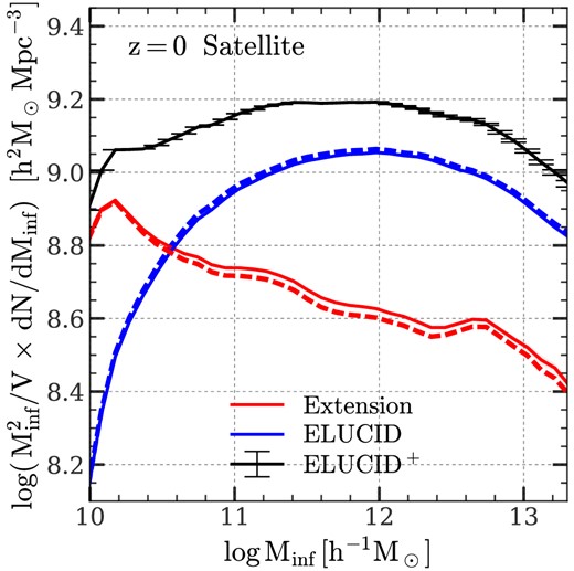
Infall mass functions of satellite subhalos selected at |$z$| = 0 in the ELUCID simulation. The blue solid line (labelled ‘ELUCID’) is the result using subhalos resolved by the original ELUCID simulation. The black solid line (labeled ‘ELUCID+’) is the result obtained from amended merger trees. For reference, the red solid line (labeled ‘Extension’) is the result for subhalos generated by the extension algorithm. A small fraction of the resolved subhalos in ELUCID is moved to ‘Extension’ to ensure a consistent halo-centric radial distribution with the high-resolution simulation, TNGDark, and the amount is the difference between the dash line (before the move) and the solid line (after the move). See Section 3.3 for a detailed description. The mass functions are multiplied by |$M^2_{\rm inf}$| for clarity. Error bars and shaded areas indicate the standard deviations computed from 50 bootstrap resamplings over halos, which are too small to see owing to the large sample size of ELUCID.
For brevity, we only show the results for subhalos at |$z$| = 0 in the main text to demonstrate the performance of our extension algorithm. Our tests showed that the extension algorithm actually works as well at high |$z$|, because the density field is less evolved and the halo population is less diverse (see Appendix A for the details).
The rest of this section is organized as follows. In Section 3.1, we outline the algorithm by listing its four steps. In Section 3.2, we describe each of the steps in general terms, so that the algorithm can be adapted to different target variables and to subhalo merger trees with different resolutions. In Section 3.3, we describe the application of the general framework to a specific case of amending subhalo merger trees of ELUCID with the use of TNGDark. For reference, Table 2 summarizes the notations of variables to be used in the description of the general framework, and Table 3 summarizes the notations in the description of the specific case of using TNGDark to amend ELUCID merger trees. Fig. 2 shows a schematic diagram of the algorithm.
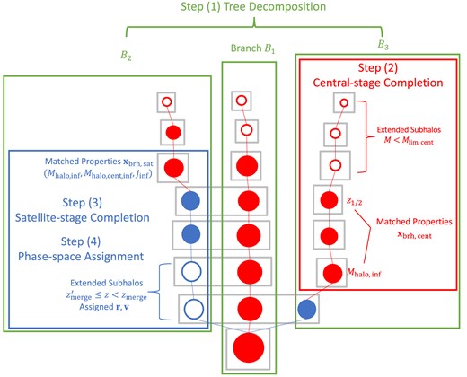
A schematic diagram of the subhalo merger tree extension algorithm, as described in Table 2 and elaborated upon in Section 3.2. Grey boxes represent halos, with red and blue circles representing central and satellite subhalos, respectively. Filled circles denote subhalos that are resolved by the simulation, while empty circles indicate subhalos that were missed and subsequently created through the extension. Subhalos processed at each step of the algorithm are enclosed within a coloured box.
Notations for variables used in the description of the extension algorithm in Section 3.2. The first column lists the location where the notation first appears. The second and third columns list the notations and their descriptions, respectively. Note that most of these are abstract variables used in the description of the general framework. The concrete choices depend on the specific application (see Section 3.3 and Table 3 for the example demonstrated in this paper).
| First appearance | Notations | Descriptions |
|---|---|---|
| Outline of the algorithm | S, S′ | The target low-resolution simulation, and the reference high-resolution simulation used as training source. |
| Tree decomposition | F, T | A forest and a subhalo merger tree. |
| Bi, ri, ci | The i-th branch obtained by decomposing a subhalo merger tree, the root subhalo of this branch, and the ‘last central subhalo’ of this branch. | |
| NB | The number of branches obtained by decomposing a subhalo merger tree. | |
| |$z$|inf, |$z$|first | The infall redshift of a whole branch or of any subhalo in this branch, and the first resolvable redshift of this branch. | |
| Central-stage completion | xbrh, cent | A set of branch properties is used to match central stages of branches. |
| dcent (B, B′) | The L2 distance between two branches B and B′ for the central stage. | |
| Mlim, cent, |$z$|joint | The halo mass threshold below which the extension is applied for a branch, and the corresponding ‘joint’ redshift. | |
| Satellite-stage completion | xbrh, sat | A set of branch properties is used to match satellite stages of branches. |
| dsat(B, B′) | The L2 distance between two branches B and B′ for the satellite stage. | |
| |$z$|merge | The redshift when a satellite subhalo merges into another subhalo. | |
| Phase-space assignment | xsat | The set of satellite properties whose joint distribution is required to be recovered when we assign properties to satellites. |
| xsat, complete, xsat, incomplete | The complete and incomplete parts of xsat that are resolved and missed by the target simulation, respectively. | |
| Imissed | A binary variable indicating whether or not a satellite is missed by the target simulation. | |
| Ci, Hi, |$N_{H_i}$| | The i-th cell obtained by partitioning the feature space of satellites, the set of satellite subhalos in this cell, and the size of this set. | |
| |$d_{\rm cell}(H_i, H_j^{\prime })$| | The L2 distance between two cells Hi and |$H_j^{\prime }$| in the match of conditioning variables. | |
| Ncell, Ncell, max | The total number of cells and its upper bound imposed by us. | |
| Nmin, cell partition, Nmin, cell match | The minimal number of satellites from S and S′, respectively, for a cell to be treated as valid. |
Summary of notations (first panel) and choices (second panel) specific to S = ELUCID and S′ = TNGDark used in Section 3.3. Some intermediate variables are not listed here. A variable that appears in both S and S′ is distinguished by a prime symbol, such as rlf and |$r_{\rm lf}^{\prime }$|.
| Notations | Descriptions |
|---|---|
| Mhalo, inf | The infall mass of a whole branch or of any subhalo (central or satellite) in this branch. |
| Mhalo, host | The mass of the current host halo of any subhalo (central or satellite). |
| Minf, sat, Mhalo, cent, inf, jinf | For any satellite subhalo, these three variables are the halo mass of it right before infall, the halo mass of the central subhalo into which it falls, and its orbital angular momentum, respectively. |
| Mmatch, cent | The threshold of Mhalo, inf below which formation time is not used for the central-stage neighbor matching. |
| |$z$|1/2 | The half-halo-mass formation redshift of a central subhalo, i.e. the redshift at which the halo mass on its main branch first exceeds half of its current halo mass. |
| rp, i, vp, i, Np | The position and velocity of the i-th particle in a halo, and the total number of particles in that halo. |
| |$\mathcal {I}$|, λi, ei, ai, si | For a halo, these give its inertial tensor, the i-th eigenvalue and eigenvector of the inertial tensor, the i-th major axis of the inertial ellipsoid, and the stretching factor along this axis, respectively (see equations 11, 12 and 14). |
| rcom, vcom | The position and velocity of the center of mass (COM) of a halo. |
| Rhalo, host, Rhalo, host | The virial radius and virial velocity of the host halo of a subhalo. |
| r, v | The position and velocity of a subhalo in real space. |
| rlf, vlf | The position and velocity of a subhalo in the local frame defined by its host halo (see equation 13). |
| rlf, θr, lf, ϕr, lf | The spherical coordinates of the local-frame position. |
| |$v$|lf, θ|$v$|, lf, ϕ|$v$|, lf | The spherical coordinates of the local-frame velocity. |
| rlf, com | For a halo, this variable gives the distance between its COM and the minimal potential of its central subhalo, both measured in the local frame. This variable is an indicator to the relaxation state of a halo. |
| Δlog rlf, max | The maximal difference in the halo-centric distance for a subhalo in S to be conditionally matched with a subhalo in S′. |
| Step | Choices |
|---|---|
| Central-stage completion | |${\boldsymbol x}_{\rm brh, cent} = \, [\log M_{\rm halo,inf},\, \log (1+ z_{1/2}) \, ]$| or log Mhalo, inf |
| |$M_{\rm match,cent}=2\times 10^{10} \, h^{-1}\, {\rm M_\odot}$|, |$M_{\rm lim,cent}=10^{10} \, h^{-1}\, {\rm M_\odot}$| | |
| Satellite-stage completion | |${\boldsymbol x}_{\rm brh, sat} = (\log M_{\rm halo, inf},\, \log M_{\rm halo, cent, inf}, \log \, j_{\rm inf})$| |
| Phase-space assignment | Ncell, max = 768, Nmin, cell partition = 32, Nmin, cell match = 32 |
| |${\boldsymbol x}_{\rm sat, complete} = [\log (1+z_{\rm inf}), \log \frac{M_{\rm inf, sat}}{M_{\rm halo, host}}, \log M_{\rm halo, host}, \ r_{\rm lf, com}]$| | |
| |${\boldsymbol x}_{\rm sat, incomplete} = \, ({\boldsymbol r}_{\rm lf},\, {\boldsymbol v}_{\rm lf})$| | |
| Δlog rlf, max = 0.1 |
3.1 Outline of the algorithm
The extension algorithm is designed to work on all subhalo merger trees in a low-resolution simulation, |$\rm S$|, by learning from another high-resolution simulation, |$\rm S^{\prime }$|. The goal is that, for any central subhalo identified in |$\rm S$|, (i) its mass assembly history (MAH) is extended to higher redshift with a mass resolution similar to that of |$\rm S^{\prime }$|, and (ii) its lifetime after infall is extended to be consistent with that expected from |$\rm S^{\prime }$|. Note that we cannot create a subhalo whose mass is always below the resolution limit of S, so that it is not identifiable in S. In Appendix B1, we examine the completeness of the extended population and the effects of these completely missed branches. The algorithm consists of the following main steps:
Tree decomposition: each subhalo merger tree in S or S′ is decomposed into disjoint branches. These branches will be used as pieces to complete trees of subhalos in both central and satellite stages described in the following two steps.
Central-stage completion: the MAH of any central subhalo, defined as the set of halo mass values in the main branch of the subhalo merger tree rooted in this subhalo, is completed down to the same mass limit as |$\rm S^{\prime }$|. With this step, the MAHs of all central subhalos in S are extended well below the mass limit of |$\rm S$|, so that empirical models applied to them can trace star formation in a galaxy to high redshift when the amount of stars formed in galaxy is insignificant. This step is decoupled from the next two steps, so that it can be skipped if the MAH of a central subhalo does not need to be extended.
Satellite-stage completion: the lifetime of a subhalo in S after the infall is extended so that it is not artificially destroyed due to the limited resolution of S. The links of subhalos in merger trees are updated to reflect the addition of subhalos generated by the extension. With this step, the number of satellite subhalos in a host halo is similar to that expected in the high-resolution simulation. Thus, empirical models applied to S will be able to describe the satellite population conditioned on host halos, such as the conditional galaxy stellar mass functions, satellite density profiles, and the one-halo terms of two-point correlation functions (TPCFs).
Assignment of phase-space coordinates to satellite subhalos: positions and velocities are assigned to all the satellite subhalos, both the original population and the population generated by the extension algorithm. In this step, subhalo properties, such as spatial position, velocity, and various properties at the time of infall, are required to be statistically recovered. Phase-space properties of satellite subhalos that are resolvable by |$\rm S$| are kept unchanged whenever possible. Properties of host halos, such as their shapes and orientations, are also preserved whenever possible. With this strategy, the algorithm retains all reliable information from the original simulation, and perform extensions only when necessary.
3.2 Details of the algorithm
3.2.1 Tree decomposition
In the tree decomposition step, we aim to split each subhalo merger tree, T, into a set of disjoint branches |$\lbrace B_i \rbrace _{i=1} ^ {N_B}$|, each consisting of a chain of subhalos that form the main branch of a root subhalo, ri ∈ Bi. Here, NB is the number of branches in T, and |$\cup _{i=1}^{N_B} B_i = T$|. The decomposition starts from a forest F = {T} that initially contains only the target tree T, and proceeds through the following substeps:
We arbitrarily take a tree, Ti ∈ F, out of the forest F, and we denote the root subhalo of Ti as ri.
We extract the main branch, Bi, of ri, out of Ti, and we add Bi into the result set of branches.
The remaining subhalos in Ti form a set of subtrees of Ti. We add all these subtrees back into F.
We go back to the first substep and proceed iteratively until F becomes empty.
For each branch, Bi, we walk through it from the root subhalo, ri, towards high redshift, until we encounter a central subhalo ci ∈ Bi. We refer to this central subhalo as the ‘last central subhalo’ of this branch, and define its redshift to be the infall redshift, |$z$|inf, of the whole branch, and of any subhalo in this branch. Other properties of the last central subhalo, such as its halo mass, the mass of the target halo into which it is merging, and its orbital angular momentum relative to the target halo, are all computed and defined as the infall properties of the whole branch and of any subhalo in this branch. We refer to the subhalo with the highest redshift on Bi as the ‘first resolvable subhalo’ of this branch, and we define its redshift to be the first resolvable redshift, |$z$|first, of this branch.
3.2.2 Central-stage completion
In the central-stage completion step, we only focus on the central part, which consists of subhalos at or before |$z$|inf of each branch. For each target branch B in the low-resolution simulation S, we search a reference branch B′ with the same infall redshift in the high-resolution simulation S′. We require that B be closest to B′ according to some matching (‘distance’) criteria (to be specified below). Such match allows subhalo properties in the history of B′ to be borrowed by its nearest-neighbour B for extensions of properties that are poorly resolved in S. This method, referred to as the nearest-neighbour matching (NNM) in the following, is, effectively, a k-nearest neighbors (kNN) regression with k = 1, a non-parametric regression capable of dealing with highly non-linear patterns in feature space of any dimensionality (e.g. Bishop 2006; James et al. 2013). The general requirement of kNN is that the distributions of properties to be matched are similar in the two data sets. In our NNM, this requirement is achieved by using only properties that are robustly determined in both S and S′, and by standardizing these properties before the matching (see Section 3.3). Based on these considerations, the match between B and B′, the truncation of B and the borrowing from B′ by B will be achieved through the following substeps:
We define a set of branch properties that can be reliably resolved for any branch in both S and S′. We denote these properties collectively as xbrh, cent and |${\boldsymbol x}_{\rm brh, cent}^{\prime }$| in the two simulations, respectively. The branch properties to use should include variables that are the most relevant to the MAH of the central part in a branch.
- For each branch B in S, we search among all branches of the same |$z$|inf in S′ to find a B′ that is closest to B. Here, the distance, dcent(B, B′), between two branches, is the L2 distance between xbrh, cent and |${\boldsymbol x}_{\rm brh, cent}^{\prime }$|, defined as(1)$$ \begin{eqnarray*} d_{\rm cent}(B, B^{\prime }) & =& \Vert {\boldsymbol x}_{\rm brh, cent}-{\boldsymbol x}_{\rm brh, cent}^{\prime } \Vert \nonumber \\ & =& \sqrt{\left({\boldsymbol x}_{\rm brh, cent}-{\boldsymbol x}_{\rm brh, cent}^{\prime }\right)^2}. \end{eqnarray*} $$
The MAH of B before a joint redshift, |$z$|joint, when its mass goes below the resolution limit, Mlim, cent, is truncated and replaced with the MAH of B′ at |$z$| > |$z$|joint. Note that the MAH of B′ is re-scaled to avoid any discontinuity around the joint redshift. Because of the difference in redshift sampling between S and S′, we linearly interpolate the MAH of B′ to the redshift needed by B. The re-scaling and interpolation are in logarithmic scale for MAH and in log (1 + |$z$|) for the redshift. After this substep, the MAH of B is extended from |$z$|first to the first resolvable redshift, |$z_{\rm first}^{\prime }$|, of B′.
A list of new central subhalos, whose halo masses are defined by the extended part of MAH, are created and attached to the tree. To be maximally compatible with S, the positions and peculiar velocities of these subhalos at |$z$|first ≥ |$z$| > |$z$|joint in the extension retain their simulated values in S. For the sake of completeness, the peculiar velocities of these subhalos at |$z_{\rm first}^{\prime } \geqslant z \gt z_{\rm first}$| in the extension are all assigned to be zero, and their spatial positions are set to the simulated position of the subhalo at |$z$|first on B. This choice for assigning phase-space coordinates has no significance, because it is not used anywhere in empirical models of galaxy formation.
By using the branches in the reference simulation S′, the extended MAHs are more precise than the method used in Chen et al. (2019) and Yung et al. (2022, 2023), where EPS-based Monte Carlo trees are used. This is due to the fact that different EPS-based methods may produce statistically different trees (Jiang & van den Bosch 2014), and EPS-based methods need to be calibrated by N-body simulations (Parkinson et al. 2007). Even with such calibration, EPS-trees may not be able to match simulated trees accurately (e.g. Chen et al. 2019).
The extension of trees in the satellite stage is more complicated and we split it into two steps. The first is to extend the lifetimes of subhalos after the infall, and the second is to assign phase-space quantities to subhalos in their host halos. The complexity comes from the fact that satellite subhalos are subject to strong environmental effects, which need to be treated properly in order to correctly predict their properties, such as lifetimes, spatial positions, and velocities. Since phase-space properties of satellite subhalos can be observed, e.g. using the TPCFs of galaxies in real and redshift space and the number density profiles of galaxies around halos (e.g. Zehavi et al. 2005; Li et al. 2006; Wang et al. 2007; Li & White 2009; Shi et al. 2016, 2018; Coil et al. 2017; Banerjee & Abel 2020, 2021; Brainerd & Samuels 2020; Meng et al. 2020; Martín-Navarro et al. 2021) it is necessary for our algorithm to recover them properly.
3.2.3 Satellite-stage completion
In the satellite-stage completion step, we focus only on subhalos at and after |$z$|inf in each branch. For each target branch B in S, the procedure is similar to the NNM adopted in the central-stage completion: we search in S′ a reference branch B′ that matches B the best in infall redshift and other properties, and we extend the lifetime of B after infall using that of B′. The details are contained in the following substeps:
We define a set of branch properties that can be reliably resolved for any branch in both S and S′, and we denote it by xbrh, sat in S, and |${\boldsymbol x}_{\rm brh, sat}^{\prime }$| in S′. Here, the set of branch properties chosen needs to be correlated with the lifetime of a satellite subhalo before it merges into another subhalo.
- For each branch B in S, we match it to a branch B′ in S′ by requiring that the L2 distance, defined asis minimized among all branches with the same |$z$|inf in S′.$$ \begin{eqnarray*} d_{\rm sat}(B, B^{\prime }) = \Vert {\boldsymbol x}_{\rm brh, sat} - {\boldsymbol x}_{\rm brh, sat}^{\prime } \Vert , \end{eqnarray*} $$
The redshift, |$z_{\rm merge}^{\prime }$|, at which B′ merges into another subhalo in S′, is compared with the redshift, |$z$|merge, at which B merges into another subhalo in S. If and only if |$z_{\rm merge}^{\prime } \lt z_{\rm merge}$|, the lifetime of B is extended to |$z_{\rm merge}^{\prime }$|.
If B is extended, a list of new subhalo is created accordingly and attached to the tree.
Once the central-stage and satellite-stage completion steps are taken, links between subhalos in merger trees of S, such as the progenitor and descendant relationships, as well as group memberships, are updated to reflect the extension.
3.2.4 Phase-space assignment
In the phase-space assignment step, we assign positions and velocities to all extended satellite subhalos in S. The phase-space properties of a satellite subhalo are expected to be correlated with other properties. For example, a satellite subhalo of earlier infall is expected to have higher probability to appear in the inner region of its host halo, while a subhalo of recent infall is expected to reside in the outskirt. Other studies have also shown that some properties at the infall time of a satellite subhalo, such as the orbital angular momentum and its mass ratio with the central subhalo, are the main factors that affect its orbital dynamics (e.g. Boylan-Kolchin, Ma & Quataert 2008). Because of these correlations, it is possible to design an algorithm that not only assigns positions and velocities randomly to satellite subhalos, but can also recover the distribution of the satellite population, p(xsat), with respect to a set of variables, xsat, such as position, velocity, and other properties.
In general, modelling the full probability density function (PDF) of xsat is challenging due to its high dimensionality. To simplify the problem, we split ΛCDMsat into two subsets of variables, xsat, complete, which can be completely resolved in S, and xsat, incomplete, which is missed for some subhalos in S and needs to be assigned. We use the following constraints in the splitting:
The incomplete set xsat, incomplete must include position and velocity, or some transformations of them, because they are missed for subhalos in the extension and are the target properties of this step.
The spatial distribution of satellite subhalos must be compliant with the constraints imposed by their host halos. For example, theoretical and numerical studies both show that halos tend to be ellipsoidal rather than spherical (e.g. Sheth, Mo & Tormen 2001; Macciò et al. 2007; Chen et al. 2020), and so satellite subhalos are also expected to have non-spherical distribution if they trace the density field in their host halos. This anisotropy are clearly seen in the distribution of simlulated satellites shown in Fig. 8. Thus, to better recover subhalo distributions in individual host halos, the extension algorithm should make use of shape information of halos, namely it should be ‘shape-preserving’.
Because many satellite subhalos are resolved in S, as can be seen from Fig. 1, the algorithm is required to retain their xsat, incomplete given by S as long as this does not break any consistency with the distribution of xsat obtained from S′. This requirement implies that the ‘retained’ subhalos are not only a statistically valid population, but also compliant to S on a per-subhalo basis. The use of properties given by S in the extension algorithm is referred to as ‘self-consistency’.
Once the split is made for xsat, we can use the product rule of probability to decompose the full PDF into two terms:
where the first and second factors, on the right-hand side, are the conditioning and conditioned terms, respectively. The first term can be estimated reliably from S as a result of the definition of xsat, complete. The conditioned term, on the other hand, is unknown from S, and has to be derived elsewhere, for example, from S′. This decomposition strategy has been widely adopted in theoretical modelling of halos and galaxies. For example, HOD models mainly target at the number of member galaxies of a host halo conditioned on the halo mass. The CLFs, conditional galaxy stellar mass functions, and conditional H i mass functions (CHIMFs) extend this and model, respectively, the distributions of galaxy luminosity, stellar mass, and H i gas mass, conditioned on halo mass (Yang et al. 2003, 2008; Zandivarez et al. 2006; Robotham et al. 2010; Zandivarez & Martínez 2011; Lan, Ménard & Mo 2016; Li et al. 2022; Meng et al. 2023). This idea is also used by Chen et al. (2019) to fix the cosmic variance at the low-stellar-mass end of the galaxy stellar mass function. The CCMD model of Xu et al. (2018) further extends the conditional distribution by including both magnitude and colour as targets. The difference in our task is that the conditioning variable xsat, complete is mutivariant, and hence, the computation and application of p(xsat, incomplete|xsat, complete) require partitions in a high-dimensional feature space. To tackle this, we design the following substeps to numerically learn the conditioned distribution from S′ and assign phase-space properties to satellites in S according to the results learned.
We compute xsat, complete for all satellite subhalos in both S and S′, and we compute xsat, incomplete for all satellite subhalos in S′ and all simulated satellite subhalos in S. In addition, for any subhalo in S, a binary variable, Imissed, is defined to indicate whether or not it is missed by the simulation and thus created in the step of satellite-stage completion.
We train a CART tree classifier (Breiman et al. 1984) that maps xsat, complete to Imissed. Here, the objective function is the misclassification rate and the training sample consists of satellite subhalos from S. So trained, the feature space of xsat, complete is partitioned into a set of subregions |$\lbrace C_i\rbrace _{i=1}^{N_{\rm cell}}$| by the CART tree, with time-integrated effects of environment naturally taken into account. Internally, the CART tree represents each subregion Ci by one of its leaf nodes, and makes prediction for a test data point according to the subregion the point is located in. In what follows, we refer to each subregion as a ‘cell’ and we use Ncell to denote the total number of cells. To alleviate the effects of overfitting due to cosmic variances, we control the fineness of the partition in the training process by limiting the number of subhalos in each cell to be no less than a minimal value, Nmin, cell partition, and the total number of cells to be no larger than a maximal value, Ncell, max.
- Satellite subhalos in S and S′ are assigned to cells according to their xsat, complete. In each cell, Ci subhalos from S and S′ are collectively denoted as Hi and |$H_i^{\prime }$|, respectively:(3)$$ \begin{eqnarray*} H_i &=& \lbrace h \in S| {\boldsymbol x}_{\rm sat, complete}(h) \in C_i \rbrace , \end{eqnarray*} $$where h denotes a satellite subhalo.(4)$$ \begin{eqnarray*} H_i^{\prime } &=& \lbrace h \in S^{\prime }| {\boldsymbol x}_{\rm sat, complete}(h) \in C_i \rbrace , \end{eqnarray*} $$
- The location of Hi (or |$H_i^{\prime }$|) in the feature space is defined by averaging xsat, complete among all subhalos in it:(5)$$ \begin{eqnarray*} {\boldsymbol x}_{\rm sat, complete}({H_i}) &=& \frac{1}{N_{H_i}} \sum _{h \in H_i} {\boldsymbol x}_{\rm sat, complete}(h), \end{eqnarray*} $$where |$N_{H_i}$| and |$N_{H_i^{\prime }}$| are the numbers of subhalos in Hi and |$H_i^{\prime }$|, respectively.(6)$$ \begin{eqnarray*} {\boldsymbol x}_{\rm sat, complete}({H_i^{\prime }}) &=& \frac{1}{N_{H_i^{\prime }}} \sum _{h \in H_i^{\prime }} {\boldsymbol x}_{\rm sat, complete}(h), \end{eqnarray*} $$
- We perform a ‘cell-matching’ that identifies, for each Hi (1 ≤ i ≤ Ncell), a closest neighbour from |$H_j^{\prime }$| (1 ≤ j ≤ Ncell). Specifically, for each cell Ci, Hi is matched with |$H_i^{\prime }$| if |$N_{H_i^{\prime }}$| is larger than a pre-defined threshold, Nmin, cell match. Otherwise, |$H_i^{\prime }$| is considered too small to provide a robust estimate of the PDF of xsat, incomplete in that cell, and we use the NNM to search for a |$H_j^{\prime }$| in another cell Cj to identify the |$H_j^{\prime }$| that is closest to Hi according the L2 distance,and has |$N_{H_j^{\prime }} \geqslant N_{\rm min, cell\ match}$|. With such cell-matching, each cell Ci is attached with a sufficiently large sample of subhalos from S′, so that we can estimate robustly the PDF, p(xsat, incomplete|Ci), conditioned in this cell. This PDF will be used as an approximation to the exact PDF p(xsat, incomplete|xsat, complete) for any xsat, complete ∈ Ci.(7)$$ \begin{eqnarray*} d_{\rm cell}\left(H_i, H_j^{\prime }\right) = \Vert {\boldsymbol x}_{\rm sat, complete}({H_i})-{\boldsymbol x}_{\rm sat, complete}\left({H_j^{\prime }}\right) \Vert , \end{eqnarray*} $$
For each cell Ci, we perform a ‘conditional abundance matching’ to assign a xsat, incomplete to each subhalo in Hi, using the properties of its closest match in |$H_j^{\prime }$|. The quantities used to match and the order of matching depend on the details of S and S′ and on the exact set of properties to be borrowed from S′ and assigned to S. Independent of the detail, the general constraints are that the conditional distribution, p(xsat, incomplete|Ci), must be recovered in Hi after the assignment, and that the assignment is shape-preserving and self-consistent, as stated at the beginning of this step.
With all these steps, an extended version of subhalo merger trees is obtained for S.
3.3 Application to ELUCID and TNGDark
In this application, we extend subhalo merger trees in S = ELUCID. Here, we first specify choices of reference simulation, computation strategies, subhalo quantities and algorithm parameters for this specific application.
As shown by van den Bosch & Ogiya (2018) with a suite of idealized simulations, satellites are easily affected by numerical defects even with large number of bound particles. They found that reliably resolving the tidal evolution of a satellite for a Hubble time on a circular orbit at 20 per cent (10 per cent) of the virial radius of the host halo requires 105 (106) particles. This is too demanding for any state-of-the-art cosmological simulation. For the problem tackled here, because we only require the satellite disruption time and phase-space properties be statistically correct in the reference simulation S′, a more relaxed condition may be sufficient. As shown by Han et al. (2016) with a suite of realistic zoom-in simulations, the number density profile for resolved satellites increases with numerical resolution and becomes convergent when Nacc, the minimal particle number of satellite at accretion, is larger than ∼103. The same conclusion was reached by Guo & White (2013) using the TPCFs of galaxies predicted by applying the subhalo abundance matching technique to a pair of simulations with different numerical resolutions. If we adopt Nacc = 103 for the least massive satellite in ELUCID (|$M_{\rm inf} \sim 10^{10} \, h^{-1}\, {\rm M_\odot}$|), the reference simulation S′ is required to have a particle mass less than |$10^7 \, h^{-1}\, {\rm M_\odot}$|. Based on these, our choice of S′ = TNGDark as the reference simulation is appropriate for extending ELUCID. In Appendix B2, we present a convergence analysis for the volume of the reference simulation. Our findings indicate that the size of the TNGDark volume is sufficiently large to encompass a representative population of (sub)halos needed for the extension algorithm.
To tackle the large data volume of ELUCID, we split the simulation box of |$(500 \, h^{-1}\, {\rm {Mpc}})^3$| volume into 5 × 5 × 5 equal-sized, non-overlapping subboxes, each with volume of |$(100 \, h^{-1}\, {\rm {Mpc}})^3$|. We run the extension algorithm for each subbox independently, and combine the resulted merger trees from all subboxes into a final data product. With such implementation, the required memory and computation costs of each subbox are reasonable for a single node of a modern computer, and the computation in different subboxes can be made parallel with a cluster of nodes.
For the central-stage completion step, we define xbrh, cent, the set of properties to be used in matching branches between S and S′, as
for all branches with Mhalo, inf ≥ Mmatch, cent, and
for all branches with Mhalo, inf < Mmatch, cent. The parameter Mmatch, cent has to be chosen so that branches with Mhalo, inf ≥ Mmatch, cent have reliable values of |$z$|1/2 in S. For S = ELUCID, we have made tests and found that |$M_{\rm match, cent} = 2 \times 10^{10} \, h^{-1}\, {\rm M_\odot}$|, the mass of about 60 N-body particles, is an appropriate choice. Similarly, we set |$M_{\rm lim, cent}=10^{10} \, h^{-1}\, {\rm M_\odot}$|, which defines the joint redshift |$z$|joint of each branch in S in extending the central part of the MAH. Because Mhalo, inf and |$z$|1/2 describe the overall amplitude and detailed shape of the MAH, respectively, our choice ensures that xbrh, cent is tightly correlated with the MAH. Our tests show that this produces a smoother transition at the joint redshift |$z$|joint for individual subhalos than the simple method used by Chen et al. (2019). Using a demarcation of infall mass at Mmatch, cent, we split branches in each of S and S′ into two subsamples. For the higher mass and lower mass subsamples of S, we use the higher mass and lower mass subsamples of S′, respectively, to accomplish the central-stage completion. To suppress the distribution shift produced by the potential discrepancy between the two simulations, we standardize xbrh, cent and |${\boldsymbol x}_{\rm brh, cent}^{\prime }$| so that they have zero mean and unit standard deviation along all dimensions before applying the NNM.
To accomplish the satellite-stage completion, we need to specify the set of branch properties, xbrh, sat, to be used to match branches between S and S′. Here, we choose
where Mhalo, inf and Mhalo, cent, inf are the infall mass of the satellite subhalo and the mass of the host halo it is falling into, respectively, and jinf is the orbital angular momentum. This choice is motivated by the fact that these properties dominate the orbital dynamics of a satellite subhalo (see, e.g. Boylan-Kolchin et al. 2008), and that these properties are numerically stable (see e.g. fig. A3 in Chen et al. 2021). Similar choices have been adopted in some previous empirical models of galaxy formation, such as those developed by Lu et al. (2014a, 2015b). As in the central-stage completion, standardization of xbrh, sat is made before applying the NNM to suppress distribution shift caused by potential discrepancy between the two simulations.
In the step of assigning phase-space coordinates to satellite subhalos, diversity of dark matter halo properties such as mass, size, shape, and orientation requires a large set of halo properties to be included in xsat, complete in order to reliably model the conditional PDF, p(xsat, incomplete|xsat, complete). Such a model is in general very complicated. Here, we simplify the problem by reducing the number of variables. To this end, we transform the phase-space properties of a satellite subhalo using the properties of its host halo, so that they are scaled by the ‘local frame’ defined by the host. By so doing, the host properties are eliminated from the conditioning variable xsat, complete, and the conditioned variable xsat, incomplete becomes dimensionless. This is, effectively, a stacking method that first scales the properties in different systems and then combines the scaled quantities to enhance the signal. This method has been used frequently in literature to extract features from weak signals, such as images or spectra with low signal-to-noise ratios.
For each host halo, we first compute its inertial tensor |$\mathcal {I}$| using
where the summation is over all the Np dark matter particles belonging to the halo, Δrp, i = rp, i − rcom is the position vector of the i-th particle relative to the centre of mass (COM), |${\boldsymbol r}_{\rm com} = \frac{1}{N_{\rm p}} \sum _i {\boldsymbol r}_{\rm p, i}$|, and mp is the mass of each particle. Then, we compute the eigenvalues, λi, and eigenvectors, ei, of the inertial tensor. We describe the shape of the halo by the principal axes, |$a_i\, (i=1,2,3)$|, of its inertial ellipsoid:
The eigenvectors and the principal axes define the local frame of the halo, to which we transform the position, r, and velocity, |$\bf v$|, of each member subhalo using
Here Rhalo, host and Vhalo, host are the virial radius and virial velocity of the host halo, respectively; |${\boldsymbol v}_{\rm com} = \frac{1}{N_{\rm p}} \sum _i {\boldsymbol v}_{\rm p, i}$| is the velocity of the COM obtained by averaging the velocities of all particles in the halo; |$\mathcal {E} = ({\boldsymbol e}_1, {\boldsymbol e}_2, {\boldsymbol e}_3)^T$| is the rotational matrix; |$\mathcal {S} = {\rm diag}(s_1, s_2, s_3)$| is the stretching matrix along the three principal axes, with the stretching factor si along the i-th principal axis defined as
To describe the radial and angular distribution of satellite subhalos in the local frame defined by the host halo, we define, for a subhalo located at rlf with velocity vlf, its halo-centric distance rlf and position angle θr, lf as
Here, Δrlf ≡ rlf − rlf, cent, and Δrlf, com ≡ rlf, com − rlf, cent, with rlf, cent and rlf, com being the local-frame positions of the central subhalo and the COM of the host halo, respectively. So defined, rlf and θr, lf are, respectively, the radial distance and polar angle in the spherical coordinate system with the polar axis parallel to Δrlf, com.
Similarly, we define the halo-centric speed |$v$|lf and velocity polar angle θ|$v$|, lf as
where Δvlf ≡ vlf − vlf, cent, and Δvlf, com ≡ vlf, com − vlf, cent. vlf, cent and vlf, com are the local-frame velocities of the central subhalo and of the COM of the host halo, respectively. Note that both rlf, com and vlf, com are zero by their definitions.
With phase-space properties defined in the local frame, we choose the properties in the conditional PDF of the phase-space assignment step as
Here, |$z$|inf and Minf, sat are the infall redshift and infall mass of the satellite subhalo, respectively, and Mhalo, host is the current mass of the host halo. The separation, rlf, com ≡ ‖Δrlf, com‖, is a quantity that measures the relaxation state of the host subhalo (see, e.g. Macciò et al. 2007; Ludlow et al. 2012; Chen et al. 2020), and is included here to control un-relaxed systems that are expected to be more asymmetric in their mass distribution (see Section 4.5 and Fig. 8 for some examples). By using rlf and vlf as target variables, the shape information of the host halo is automatically included. In some cases, for example, when simulating an extremely large volume or simulating a large ensemble of volumes, storing the full catalogue of dark matter particles into disc is infeasible. Then, we can simply remove the shape information and degrade the local frame (equation 13) to a spherically symmetric coordinate system. Our tests show that, with this simplification, the shape-preserving feature is lost, but spherically averaged summary statistics, such as the number density profiles for satellites and the TPCFs for subhalos, are still precisely corrected by the extension algorithm.
When using the CART tree to split the feature space of xsat, complete in cells, we need to specify a stopping criterion for the recursive space partitioning. Throughout this paper, we set Ncell, max = 768 and Nmin, cell partition = 32, which gives the upper bound of the number of cells and the lower bound of the number of satellite subhalos in each cell, respectively. We have made tests by allowing a relatively large Ncell, max, and found that the partition of feature space is sufficiently fine to reproduce the joint distribution of satellite properties we are interested in. By limiting the minimal cell size, the uncertainties caused by the cosmic variance can be controlled effectively, thus making the extension more stable. With a similar consideration, we set Nmin, cell match = 32, which gives the lower bound of the number of satellites from S′ in the matched cell. Note that these values are specific to the simulations used here, and should be tested when applying the method to other data sets.
Fig. 3 shows the distribution of satellite subhalos from the first subbox of ELUCID in projected spaces of the conditioning variable xsat, complete. Subhalos in several largest cells are plotted using coloured points. In all 2D panels, cells are regular rectangles because of of the bi-partition nature of the CART tree classifier. The 1D distribution of the host halo mass, log Mhalo, host, shows a concentration at |$10^{14} \, h^{-1}\, {\rm M_\odot}$|, indicating a significant cosmic variance in the ELUCID subbox used here. Several largest cells, such as those coloured with cyan, orange, yellow and purple, are located in this concentration. This indicates that the classifier captures this special population of satellites in massive halos where environmental effects are strong, and allocates individual cells to them. Some horizontal strips are clearly seen in the 2D plots, because massive halos are rare and all satellites in one such halo share the same Mhalo, host and rlf, com. Cells are well separated in the 2D panels along the axes of log (1 + |$z$|inf), |$\log \frac{M_{\rm inf, sat}}{M_{\rm halo, host}}$| and log Mhalo, host, indicating the importance of these variables in predicting numerical defects indicated by Imissed (see, e.g. Bosch et al. 2018; Green et al. 2021). This is expected, because environmental processes, no matter physical or numerical, have time-integrated effects that depend on the potential of the satellite itself, the density and tidal strength of the host halo, and the time duration since the infall. In contrast, significant overlaps of cells are seen along the axis of rlf, com, indicating that incomplete relaxation of host halos has a more subtle effect on satellite dynamics.
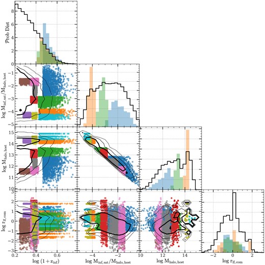
Marginal distributions of |$z$| = 0 ELUCID satellite subhalos in the projected spaces of properties that are used as the conditioning variables in the phase-space assignment step (see Table 3 and Section 3.3 for details). Satellite subhalos that are resolved by ELUCID and created in the satellite-stage completion step are both included. Each diagonal panel shows the 1D distribution of a property. Each off-diagonal panel shows the distribution of a pair of properties. In each diagonal panel, the black histogram shows the distribution of all satellite subhalos while a coloured histogram show the distribution of subhalos in a cell found by the CART tree. Only the biggest three cells are shown. The histograms are arbitrarily normalized for clarity. In each off-diagonal panel, the black thick solid, thin solid, and dotted lines are contours enclosing 50, 75, and 90 per cent of all satellite subhalos, respectively. Dots with the same coluor represent subhalos belonging to the same cell. The biggest 10 cells are shown.
Finally, we specify our choice to rank order features used in the conditional abundance matching. We choose the halo-centric distance, rlf, as the target variable to match, because radial distributions of satellite subhalos in their host halos are the main targets we want to reproduce, and because the polar angle, θlf, is not significantly correlated with rlf, as seen from Fig. 5 that will be described in detail later. With this choice, the matching algorithm proceeds for each cell Ci in the following substeps:
- We collect the set of rlf values from all ELUCID-simulated satellite subhalos that fall into the cell, and denote it as R:Similarly, the set of rlf values in the matched cell from TNGDark is denoted as R′:(18)$$ \begin{eqnarray*} R = \lbrace r_{\rm lf}(h)\, |\, h \in H_i\ {\rm and} \ I_{\rm missed} = 0 \rbrace . \end{eqnarray*} $$(19)$$ \begin{eqnarray*} R^{\prime } = \lbrace r_{\rm lf}(h)\, |\, h \in H_j^{\prime } \rbrace . \end{eqnarray*} $$
We re-sample R′ so that the size of the re-sampled set is equal to the size of Hi. If the original size of R′ is less than required, the resampling has replacement; otherwise, it does not.
- For each simulated ELUCID satellite with a halo-centric distance rlf ∈ R, we match it with a TNGDark satellite that has a halo-centric distance rlf′ ∈ R′, requiring thatwhere Δlog rlf, max limits the matching range and is set to be 0.1. The matching starts from the most massive satellite, as measured by Minf, sat, in ELUCID, to the least massive one. If multiple satellites are found in TNGDark for an ELUCID satellite, the one with the smallest Δlog rlf is selected. Once a match is found, the matched satellite in TNGDark is removed from R′; otherwise, no match is made, and we continue with the next ELUCID satellite.(20)$$ \begin{eqnarray*} {\rm \Delta }\log r_{\rm lf} \equiv |\log \, r_{\rm lf}-\log \, r_{\rm lf}^{\prime }| \leqslant {\rm \Delta }\log r_{\rm lf, max}. \end{eqnarray*} $$
For each ELUCID satellite that is matched with TNGDark satellite, we set its phase-space properties, (rlf, vlf), to the simulated values in ELUCID. We refer to these satellites as ‘ELUCID satellites’, and their mass function is shown by the blue solid line in Fig. 1. For comparison, the blue-dashed line in that figure accounts for all satellites resolved in ELUCID without regard to the matching.
For the remaining ELUCID satellites, either created in the satellite-stage completion step or unmatched to any TNGDark satellite in the previous substep, we randomly match them, one-to-one, with TNGDark satellites that have |$r_{\rm lf}^{\prime }$| values in R′. We use (rlf, θr, lf) and (|$v$|lf, θ|$v$|, lf) from the matched TNGDark subhalo, together with randomly generated azimuthal angles ϕr, lf and ϕ|$v$|, lf (respectively, for the position and velocity) to obtain the local-frame coordinates (rlf, vlf) for each of the remaining ELUCID satellites. These ELUCID satellites are referred to as the population of extension, and their mass function is shown by the red solid line (labelled ‘Extension’) in Fig. 1. For comparison, the red-dashed line is the result for satellites that are created in the step of satellite-stage completion.
Once an ELUCID satellite subhalo is assigned values of (rlf, vlf) either directed by the target simulation or by the extension algorithm, its physical coordinates in phase-space can be obtained by inverting the transformations represented by equation (13).
4 TESTING THE PERFORMANCE OF THE EXTENSION ALGORITHM
The extension algorithm developed above produces subhalo merger trees that are more complete in MAH for both the central and satellite subhalo populations. Because the extension is shape preserving and self-consistent, the trees also retain important information contained in the original, target simulation. In this section, we present various testing results to demonstrate the reliability and accuracy of the extension algorithm.
4.1 MAHs of central subhalos
The central-stage completion step (Section 3.2.2) of our algorithm completes the assembly histories of central subhalos at high redshift when their masses are too small to be resolved in the target simulation. Fig. 4 compares the MAHs obtained from the target simulation (ELUCID), the extended version of it (|$\rm ELUCID^+$|), the reference simulation (TNGDark), and the hydro counterpart of the reference simulation (TNG). The leftmost panel shows the average MAHs of branches with |$z$|inf = 0 in three bins of halo masses at |$z$| = 0. We can understand the result using a series of pair-wise comparisons. First, the MAHs of TNG are almost indistinguishable from those of TNGDark up to |$z$| ∼ 10. This indicates that the overall halo properties, such as the virial mass and the virial radius, are stable against baryonic effects. This stability forms the basis for empirical models built on DMO simulations. Second, significant discrepancy can be seen between TNGDark and ELUCID at |$z$| ≳ 2. Above this redshift, the average MAHs of ELUCID are gradually dominated by unresolved, low-mass subhalos whose MAHs are padded artificially. Thus, an empirical model based on the MAHs of such incomplete histories will miss star formation in low-mass halos at high redshift. Finally, with the central-stage completion, the average MAHs of |$\rm ELUCID^+$| become consistent with the high-resolution simulation TNGDark over the entire redshift range shown. This indicates that our NNM-based extension produces unbiased MAH in the full redshift range up to |$z$| ∼ 10. The standard deviations of the MAHs in ELUCID, shown by the blue-shaded areas, are larger than those in TNGDark, even at low |$z$|. This is a result of the variation in the first resolvable redshift, |$z$|first, of ELUCID branches.
MAHs of central subhalos at |$z$| = 0 in different simulations. Curves are shown with different offsets for clarity. The leftmost panel shows the average histories of subhalos in three bins of |$M_{\rm halo,z=0}/(\, h^{-1}\, {\rm M_\odot})$|, indicated above each bunch of curves. Green, blue, red, and black lines are mean values from TNG, ELUCID, |$\rm ELUCID^+$|, and TNGDark, respectively, with black error bars and blue-shaded areas indicating the corresponding standard deviations among branches. The right three panels show the assembly histories of individual subhalos randomly selected in three bins of |$M_{\rm halo, z=0}/(\, h^{-1}\, {\rm M_\odot})$|, respectively, indicated at the top of the panels. For each subhalo, blue line shows its assembly history before the central-stage completion, which is truncated near the resolution limit of ELUCID. The red line shows the result after extension, which smoothly continues to the mass limit defined by the reference simulation, TNGDark.
The right block of three panels in Fig. 4 shows the MAHs of individual branches randomly selected in three different mass bins at |$z$| = 0. The MAHs resolved by ELUCID are all truncated at some redshifts when their masses are below the resolution limit of ELUCID. In contrast, the MAHs after the extension, labelled as |$\rm ELUCID^+$|, start to deviate from those of ELUCID at some joint redshifts |$z$|joint, but extend smoothly to higher redshift, eventually being truncated as their mass goes below an effective mass limit defined by TNGDark. We note that the smoothness around |$z$|joint is a combined outcome of the discontinuity-removal applied in the substep (iii) of the central-stage completion, and the specific choice of xbrh, cent made for ELUCID (see equation 8). In the history, central subhalos can fall into neighboring halos, temporarily becoming satellites, before being ejected back to the central phase. During their temporary satellite phase, we represent their halo mass by their mass right prior to infall, causing a discontinuity in the MAHs of some central subhalos, as shown in the right block of Fig. 4. These MAHs exhibit temporary plateaus, followed by sudden jumps to higher masses. Many of these infall-ejection events are artificial, arising from the bridging effect of the FoF algorithm (e.g. Klypin, Trujillo-Gomez & Primack 2011). To mitigate this issue, one can simply replace the halo finder with an algorithm that more robustly excludes these artificial links (e.g. Klypin & Holtzman 1997; Knollmann & Knebe 2009; Planelles & Quilis 2010; Behroozi et al. 2012; Vallés-Pérez et al. 2022).
4.2 Joint distribution of satellite properties
As described in Section 3.2.4, the goal of the phase-space assignment step is to recover the joint distribution of a given set of properties, xsat, of satellite subhalos. Fig. 5 shows the marginal distributions of satellite subhalos at |$z$| = 0 in the space of various properties. The subhalo properties presented in the figure are the halo-centric radial distance rlf and the polar angle θr, lf, both defined with respect to the local frame of the host halo, the infall mass Minf, sat, scaled either by Mhalo, host, the current host halo mass, or by Mhalo, cent, inf, the mass of the host halo into which it fell at |$z$|inf, the infall redshift |$z$|inf, and the infall orbital angular momentum jinf. In the 1D distributions of rlf, θr, lf, Minf, sat/Mhalo, host and |$z$|inf, the reference simulation, TNGDark, shows significant differences from the target simulation, ELUCID. The difference between the PDF of the two simulations is quantified by the Kolmogorov–Smirnov (K-S) statistic, which is larger than 0.1 in each of these four panels. These differences are expected and can be interpreted as follows. First, a satellite in ELUCID is more likely disrupted artificially in the inner region of its host halo, because of the denser environment in that region and the long time-integration before arriving there. This causes a shift of the PDF towards larger halo-centric distance as seen in the 1D panel for rlf. The density profiles and correlation functions presented in Figs 6, 7, and 9 also show the effects of such incompleteness in ELUCID. Secondly, the distribution of satellites resolved in ELUCID tends to align in the direction of the COM, as seen from the 1D PDF of cos θr, lf. This is partially due to our choice for the polar direction of the spherical coordinate system used in equation (15), and partially due to the stronger environmental effect on satellites that are closer to xlf, cent, the location of the local potential minimum in the host halo. Thirdly, a satellite with lower infall mass has shallower local gravitational potential to prevent its matter from environmental disruption, especially when it approaches the halo center. As a result, the PDF of the ratio Minf, sat/Mhalo, host for ELUCID is shifted towards higher values of the ratio. Finally, the shift of the PDF of |$z$|inf towards smaller values in ELUCID is a result of the time-integration of numerical loss. Unlike Minf, sat/Mhalo, host, the PDF of Minf, sat/Mhalo, cent, inf for ELUCID shows no significant difference from that for TNGDark. This is a coincidence produced by the left-shifted PDF of |$z$|inf, the right-shifted PDF of Minf, sat/Mhalo, host, and the positive correlation between |$z$|inf and Minf, sat/Mhalo, cent, inf.
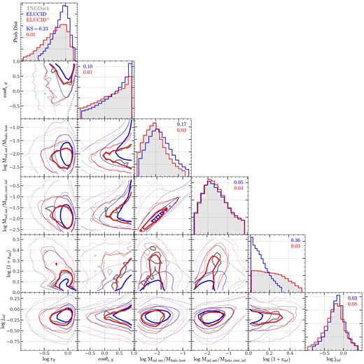
Marginal distributions of satellite subhalos in the projected spaces of several properties as indicated by legends of individual axes. Satellite subhalos in host halos with |$M_{\rm halo, host} \in [10^{12}, 10^{13})\, h^{-1}\, {\rm M_\odot}$| at |$z$| = 0 are used in the plot. Each diagonal panel shows the 1D distribution of a property. Each off-diagonal panel shows the 2D distribution of a pair of properties. The grey, blue, and red histograms or contours are the distributions of subhalos in TNGDark, ELUCID, and |$\rm ELUCID^+$|, respectively. In each off-diagonal panel, the thick solid, thin solid, and dotted lines enclose 30, 60, and 90 per cent of subhalos, respectively.
Summary statistics for spatial distribution of subhalos at |$z$| = 0. In all panels, black, blue, and red symbols are results from TNGDark, ELUCID, and |$\rm ELUCID^+$|, respectively. Green curves in the last row are results from the TNG hydro simulation to demonstrate the effects of baryonic processes. Error bars and shaded areas indicate the standard deviations around the corresponding mean values computed from 50 bootstrap samples. The first row shows the number density profiles, ρN, of satellite subhalos in host halos with different masses, |$M_{\rm halo,host}/(\, h^{-1}\, {\rm M_\odot})$|, indicated at the top of panels. For each given halo mass range, satellite subhalos in three different infall mass ranges are shown by solid, dashed, and dotted lines, respectively, and they are shown in an increasing 1dex vertical offset for clarity. The second row shows the angular distributions of satellite subhalos (see equation 15 and texts around it for the definition of the position polar angle θr, lf) in host halos with different masses, |$M_{\rm halo,host}/(\, h^{-1}\, {\rm M_\odot})$|, indicated at the top of panels. The K-S statistic is computed and indicated in the upper left-hand corner of each panel for the ELUCID (or |$\rm ELUCID^+$|) distribution with respect to the TNGDark distribution in the same panel. The third row shows the distributions of axis ratios of halos with different masses, |$M_{\rm halo,host}/(\, h^{-1}\, {\rm M_\odot})$|, indicated at the top of panels. The axis ratio of each halo is computed by using all subhalos (central and satellite) in this halo, weighted by their infall masses. The K-S statistics are also indicated in the upper left-hand corner of each panel. The fourth row shows the two-point autocorrelation functions of all subhalos (central and satellite) in subsamples with different infall masses, |$M_{\rm inf}/(\, h^{-1}\, {\rm M_\odot})$|, indicated at the top of each panel.
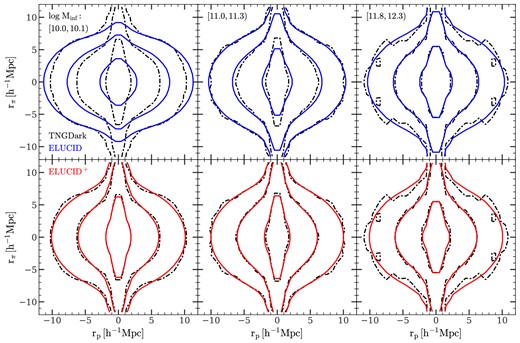
Two-dimensional correlation functions ξ(rp, r|$_{\pi}$|) in redshift space for subhalos (central plus satellite) at |$z$| = 0. Three columns show the results for halos with different infall masses, |$M_{\rm inf}/(\, h^{-1}\, {\rm M_\odot})$|, indicated in the top left-hand corner of the panels in the first row. Black contours in all panels are obtained from TNGDark. Red and blue contours in two rows are obtained from ELUCID and its extended version, ELUCID+, respectively.
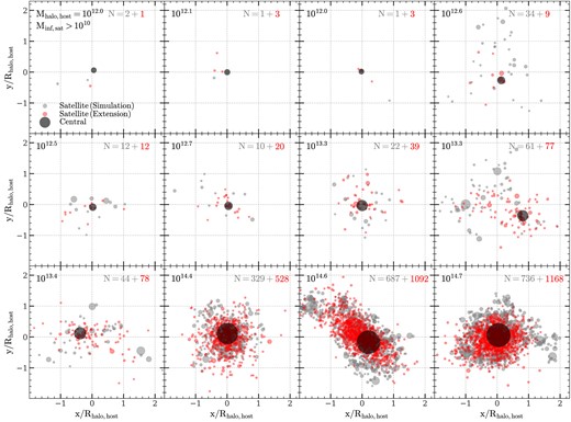
Subhalo distributions in the real space of several example halos in ELUCID. Each panel shows the subhalos in one host halo whose mass, |$M_{\rm halo,host}/(\, h^{-1}\, {\rm M_\odot})$|, is indicated in the top left-hand corner of that panel. Black, grey, and red dots represent central subhalo, satellite subhalos resolved by ELUCID, and satellite subhalos generated by the extension algorithm, respectively. All subhalos with mass greater than |$10^{10} \, h^{-1}\, {\rm M_\odot}$| are shown. Radius of a dot is proportional to the square root of the subhalo infall mass, Minf. The numbers of simulated and extended satellite subhalos are separately indicated in the upper right-hand corner of the panel. The origin of each panel is the COM of the host halo, computed by using all the particles linked to it.
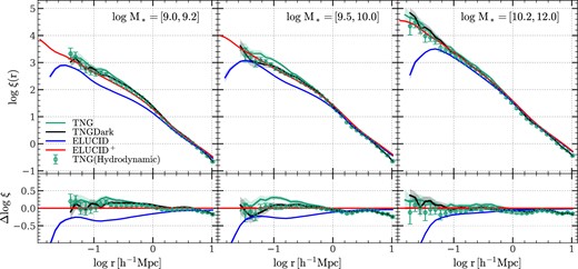
Real-space correlation functions of |$z$| = 0 galaxies with different stellar masses indicated in the top right-hand corner of each panel. These galaxies are obtained by applying a halo-based empirical model adapter, MAHGIC, to four versions of subhalo merger trees. Green, black, blue, and red solid curves are the results of the empirical model implemented with subhalo merger trees in TNG, TNGDark, ELUCID, and |$\rm ELUCID^+$|, respectively. Green dots are results of the simulated galaxies from the TNG simulation. The first row shows the correlation functions ξ(r), and the second row shows the difference of each correlation function with respect to |$\rm ELUCID^{+}$| in the same range of stellar mass. The shaded areas and error bars represent the standard deviations computed from 50 boostrap samples.
The 2D marginal distributions in Fig. 5 present more demanding tests on satellite properties predicted by ELUCID. The discrepancy between ELUCID and TNGDark is even worse in these distributions. Indeed, none of these panels shows consistent contours between the two simulations. This discrepancy indicates that a halo-based galaxy formation model applied to ELUCID will not be able to predict reliably the spatial distribution of satellite galaxies and the joint distribution between spatial positions and other properties of satellite galaxies.
Thus, extensions of the satellite parts of subhalo merger trees are clearly needed by ELUCID. To this end, we separate the difference between ELUCID and TNGDark in the joint distribution of satellite properties into two parts. In the first part, the difference is the amplitude of the distribution function caused by the inadequate number of satellites resolved by ELUCID up to the epoch in question. In the second, the difference is the shape of the distribution function caused by the dependency of artificial disruption on other satellite properties. The two parts of the difference are corrected, separately, by two steps of our algorithm, the satellite-stage completion (Section 3.2.3) and the phase-space assignment (Section 3.2.4).
The red histograms and contours labelled as |$\rm ELUCID^+$| in Fig. 5 show the 1D and 2D marginal PDFs, respectively, of satellite properties after the application of the extension algorithm. In the 1D panels, the discrepancy seen between ELUCID and TNGDark is completely absent between ELUCID+ and TNGDark. The K-S statistics between them in all panels are now below 0.1, indicating small difference between the two sets of the data after the amendment using the extension algorithm. The consistency between ELUCID and TNGDark in 2D distributions is also improved significantly after the amendment, as can be seen from the similarity in contours between ELUCID+ and TNGDark. Remarkably, in the space of each pair of variables considered here, |$\rm ELUCID^+$| follows TNGDark closely even in their 90 per cent contours. The angular distribution, as represented by panels showing pairs that contain θr, lf, is also well recovered, even though we only used the radial distance, rlf, as the quantity to match in the conditional abundance matching step. This is at least partly because of the correlation between θr, lf and other conditioning variables. Although Fig. 5 shows only a specific host halo mass range, our tests showed that the recovery of the distribution of satellite properties in all other halo mass ranges is as good as or even better than the results presented here. Our tests also showed that the algorithm performs equally well for halos identifies at |$z$| > 0 (see Fig. A2 for an example). At high redshift (|$z$| ≳ 4), the sample size of massive halos (|$M_{\rm halo, host} \gtrsim 10^{12} \, h^{-1}\, {\rm M_\odot}$|) in TNGDark is too small to be robustly compared with ELUCID for the joint distribution. In this case, the split of the full set of satellite properties into conditioning and conditioned sets, and the lower bounds we impose on Nmin, cell partition and Nmin, cell match in partitioning the feature space and matching cells, respectively (see Section 3.2.4), are the keys to suppressing the cosmic variance and to achieving a robust assignment of phase-space coordinates.
4.3 Summary statistics of the subhalo population
The recovery of the joint distribution in space of high-dimensionality indicates that other statistical properties of the subhalo population are also recovered. For completeness, Fig. 6 shows four statistical measurements that are commonly used in literature. The first row of Fig. 6 shows the number density profile, ρN, as a function of the halo-centric distance r measured relative to the central subhalo and scaled by the virial radius, Rhalo, host, of the host halo. Results are shown for satellite subhalos with different infall masses, Minf, sat, and in host halos with different masses, Mhalo, host. From curves showing TNGDark results, it is clear that the overall amplitude of ρN is larger for more massive host halos and for less-massive satellites. HOD models (e.g. Jing et al. 1998; Berlind & Weinberg 2002; Guo et al. 2015, 2016; Qin et al. 2022; Yuan et al. 2022) are usually parametrized with this assumption. The profile decreases monotonically with increasing halo-centric distance, which is usually modelled by a double-power-law form, such as the NFW (Navarro et al. 1997) profile. With limited resolution, the profiles revealed by the ELUCID simulation, as shown by blue curves, lack some of these critical features. The profiles of ELUCID follow those of TNGDark at large radii, but they start to bend down when approaching to inner regions of host halos. For satellite subhalos with masses |$\sim 10^{10} \, h^{-1}\, {\rm M_\odot}$|, the profiles start to deviate from those of TNGDark even at r ∼ Rhalo, host. Very few subhalos of such mass are present at r < (1/5)Rhalo, host. These subhalos have masses too close to the mass resolution limit of ELUCID, and are severely affected by numerical artefacts. More massive satellite subhalos in ELUCID are more stable against numerical effects, but they are also underrepresented in the inner region of the hosts, because their progenitors and structures may not be properly resolved. The profiles after extension, marked as ELUCID+ and shown by red curves, are significantly improved. Over the entire ranges of both the host halo mass and the satellite infall mass, the extended profiles follow tightly those of TNGDark all the way to r ∼ 0.1Rhalo, host. At r < 0.1Rhalo, host, the TNGDark profiles become noisy, as seen from the large fluctuations and error bars. However, the ELUCID+ profiles in the innermost regions, r ∼ 10−1.5Rhalo, host, are still stable, owing to the much larger simulation volume and sample size of ELUCID in comparison to TNGDark. Note that training of the extension algorithm is less demanding on sample size than some statistical measures. These results indicate that our extension algorithm is able to combine the large volume of the target simulation with the high resolution of the reference simulation.
When modelling galaxy formation based on subhalos, the number density profiles of satellite galaxies serve as a critical test or calibration for model predictions. These profiles provide the ‘one-halo’ terms in galaxy TPCFs, which can be measured directly from galaxy surveys (e.g. Li & White 2009; Meng et al. 2020). With a halo-based group finder (see, e.g. Yang et al. 2005, 2007; Wang et al. 2020), these profiles can also be measured directly by stacking groups of similar masses and by properly correcting redshift-space distortions (RSDs). Thus, the extension algorithm developed here provides a solid basis to model galaxy clustering reliably.
The second row of Fig. 6 shows the angular distribution of satellite subhalos in terms of the PDF of the cosine of the position angle θr, lf in host halos of different masses. The PDFs all have a minimum at θr, lf ∼ |$\pi$|, increase as the polar angle decreases, and reach to a maximum at θr, lf ∼ 0. This tendency of alignment between the halo COM and satellites is an outcome of our definition of the spherical coordinate system in the local frame (see equation 15). The alignment is stronger in lower mass host halos and particularly significant in halos with |$M_{\rm halo, host} \lt 10^{12} \, h^{-1}\, {\rm M_\odot}$|. This is because lower mass hosts have a smaller number of satellites, which are preferentially distributed around the COM. With a limited resolution, ELUCID misses some of the satellites, and the missed fraction is more significant for satellites that are anti-aligned with the COM and in less-massive hosts. By the definition of the polar angle, these anti-aligned satellites are closer to the central subhalo on average and have smaller mass to resist numerical noise as they approach the potential minimum. After the extension, the PDFs obtained from ELUCID+ become indistinguishable from those of TNGDark, indicating that our algorithm successfully captures the angular distribution of satellites. The K-S statistic, which measures the difference between the PDFs of two distributions, is >0.1 between ELUCID and TNGDark for host halos with |$M_{\rm halo, host} \lt 10^{12.8} \, h^{-1}\, {\rm M_\odot}$| and becomes negligibly small (≤0.02) between ELUCID+ and TNGDark.
The third row of Fig. 6 shows the distribution of the axis ratio for halos with different masses. Following Macciò et al. (2007) and Chen et al. (2020), we use the definition
where q1, q2, and q3 are the three principal axes of the inertial ellipsoid computed using all member subhalos (central and satellite) weighted by their infall masses. So defined, a spherical halo has qaxis = 1 while a needle-shaped halo has qaxis = 0. Compared with TNGDark, halos in ELUCID tend to be slightly more elongated, as seen in the first three bins of halo masses. This is likely caused by the higher odd of disrupting underresolved subhalos in inner regions of ELUCID halos combined with the fact that the distribution of satellite subhalos tends to be more spherical in inner regions of their hosts. After the extension, the distributions of qaxis become more like those in TNGDark. This is a result of the shape-preserving nature of our algorithm together with the recovery of subhalos in the inner regions of host halos. The K-S values after the extension are reduced for halos with |$M_{\rm halo, host} \in [10^{12}, 10^{13.3}) \, h^{-1}\, {\rm M_\odot}$|, but slightly increased for halos with |$M_{\rm halo, host} \lt 10^{12} \, h^{-1}\, {\rm M_\odot}$| and |$M_{\rm halo, host} \geqslant 10^{13.3} \, h^{-1}\, {\rm M_\odot}$|. The slightly worse K-S for the lowest mass halos is caused by the small number of satellites in elongated distribution, as seen from the long tail of the PDF at qaxis ∼ −2. For halos in the highest mass bin, the TNGDark sample is small, and the reference distribution it provides is uncertain, as one can see from the shape of its histogram.
The position polar angle θr, lf and the axis ratio qaxis are two quantities that can be used to describe the anisotropic distribution of satellites in host halos. The anisotropic distribution of satellites, and its dependence on properties such as colour and quenching state, have been detected in observations and tested using simulations (see e.g. Yang et al. 2006; Ibata et al. 2013; Brainerd & Samuels 2020; Martín-Navarro et al. 2021). Because our extension algorithm is shape-preserving and can recover the anisotropic distribution of satellite subhalos, halo-based models using the extended trees are expected to be able to reproduce the anisotropic distribution, and can be used to separate effects produced by the underlying subhalo distribution from those generated by baryonic processes.
The last row of Fig. 6 shows the TPCF ξ(r) of subhalos (central and satellite) with different infall masses, where r is the separation of subhalo pairs. Much like the density profile, the ‘one halo’ term of ξ(r) is underestimated by ELUCID due to missed subhalos, and its deviation from TNGDark becomes more significant in the inner region of host halos. Subhalos with larger infall masses in ELUCID are less affected by numerical defects, and their ξ(r) follows that of TNGDark better. After the extension, the discrepancy is almost completely removed, as one can see by comparing ELUCID+ with TNGDark. The extension allows ξ(r) in the low-resolution target simulation to be extended accurately to very small scales. Note also that the amended correlation functions (red lines) are much smoother than their counterparts in TNGDark (black lines) on scales below |$0.1 \, h^{-1}\, {\rm {Mpc}}$|, again because of the difference in sample size. Complementary to the density profile of satellites, the correlation function carries additional information about clustering on interhalo scales. Since our extension algorithm does not change the ‘two-halo’ term, the small differences between ELUCID+ (or ELUCID) and TNGDark on such scales are due partly to the difference in cosmological models adopted in the two simulations and partly to cosmic variances in TNGDark. These differences can be removed by using identical cosmology for both the target and reference simulations, S and S′, and by taking into account cosmic variances caused by the smaller volume of the reference simulation. In Appendix B, we assess the performance of the extension algorithm by employing a pair of simulations with identical cosmological parameters and initial condition. Notably, the differences in the TPCFs at large radii are effectively removed, as seen from the darkest orange line and the black line in Fig. B3.
It is known that baryonic processes can affect the underlying dark matter distribution. The baryon component tends to make subhalos more concentrated and thus harder to strip by tidal forces in their host halos. The difference in the mass that can be retained by a subhalo can, in turn, change the orbit of the subhalo. However, the distribution of the baryonic component is sensitive to the subgrid physics implemented in a hydro simulation, and its effects are difficult to quantify in a unified way. For example, combining hydrodynamic simulations and subhalo abundance matching models, Simha et al. (2012) showed that the TPCF of galaxies is affected by mass contained in stars, and that the existence of momentum-driven winds in hydrodynamic simulations can modify effects of the baryonic component. As a test, we compute the TPCFs from TNG, the full hydro counterpart of TNGDark, and show the results by green curves in the last row of Fig. 6. The difference between TNGDark and TNG is much smaller than that caused by numerical resolution as measured by the difference between TNGDark and ELUCID, and it is comparable to the uncertainty of our extension algorithm as measured by the difference between TNGDark and ELUCID+. This indicates that our extension algorithm has nearly reached the upper limit of the quality provided by the high-resolution DMO simulation that does not include baryonic effects. To include baryonic effects in our modelling, a simple solution is to keep the extension algorithm unchanged, but to replace the training simulation, S′, with a hydro simulation that implements baryonic processes. This solution, however, will depend on baryonic processes implemented in and the accuracy of the hydro simulation.
4.4 Redshift-space correlation functions
Tests presented above are based on positions of subhalos, and it is clearly important to check how the extension algorithm performs on modelling peculiar velocities of subhalos. Accurate phase-space information is critical to generating reliable mock galaxy samples that mimic the real observations in redsift space. In redshift space, the line-of-sight (LOS) peculiar velocities of subhalos distort the pattern of galaxy clustering in space, which is known as the Finger of God (FOG) effect on small scales (Jackson 1972; Fisher et al. 1994), and the Kaiser effect on large scales (Kaiser 1987). The RSD caused by the FOG effect depends on the density and velocity profiles of subhalos in their host halos, and so low-resolution simulations may not be able to model it accurately.
To see the effect of numerical resolution on RSD, we compute the two-dimensional correlation function, ξ(rp, r|$\pi$|), as a function of the projected separation, rp, and the LOS separation, r|$\pi$|, for pairs of subhalos. The results of TNGDark and ELUCID are shown in the first row of Fig. 7 for subhalos (central and satellite) of different infall masses. Here, we use the |$z$| = 0 snapshot and choose the |$z$|-axis of the simulation box as the LOS direction. For low-mass subhalos with |$M_{\inf }\sim 10^{10} \, h^{-1}\, {\rm M_\odot}$|, the FOG effect is severely suppressed in ELUCID, as seen from the less elongated contours of ξ(rp, r|$\pi$|). This is expected, because a lower mass satellite has a larger probability to be artificially destroyed in ELUCID due to the limited resolution, as seen from the first row of Fig. 6. In contrast, subhalos with higher masses, such as those with |$M_{\rm inf} \sim 10^{12} \, h^{-1}\, {\rm M_\odot}$|, are less likely to be missed, and their RSD patterns in ELUCID follow better those in TNGDark.
The two-dimensional correlation function of the extended population with reassigned phase-space coordinates are shown in the second row of Fig. 7. Comparing with the original ELUCID results, we see that the discrepancy with TNGDark for low-mass subhalos is completely removed and that the contours of ξ(rp, r|$_{\pi}$|) from ELUCID+ match well with their TNGDark counterparts. For high-mass subhalos, the improvement is still evident but less remarkable, because of the smaller difference between ELUCID and TNGDark to start with. Overall, ELUCID+ results match those of TNGDark very well. Contours of ELUCID+ are significantly smoother, again because of the significantly larger simulation volume of ELUCID.
4.5 Subhalos in individual halos
As a visual inspection, Fig. 8 shows some examples of the spatial distributions of satellites in individual halos randomly picked from the population of |$M_{\rm halo, host} \geqslant 10^{12} \, h^{-1}\, {\rm M_\odot}$|. The central, simulated, and extended subhalos are presented by symbols of different colours. The numbers of simulated and extended satellites are listed in each panel. The number of satellites with infall mass above |$10^{10} \, h^{-1}\, {\rm M_\odot}$| is usually smaller than 10 for halos of |$~10^{12} \, h^{-1}\, {\rm M_\odot}$|, less than 100 for halos with mass |$~10^{13} \, h^{-1}\, {\rm M_\odot}$|, and over 1000 for the largest halos with mass |$\gt 10^{14.5} \, h^{-1}\, {\rm M_\odot}$|. Over the entire range of host halo mass, a non-negligible fraction of satellites is not properly resolved by the ELUCID. The missed satellites are comparable to the simulated ones in their total number, but are usually less massive, as seen from the smaller symbol sizes. This is consistent with the number density profiles shown in the first row of Fig. 6. Note that phase-space coordinates of most of the simulated satellites are preserved and assignment is made mainly for low-mass satellites that are not properly resolved by ELUCID. This is an outcome of the ‘self-consistency’ strategy in the conditional abundance matching step (see equation 20 and the texts around it) intended to preserve as much as possible the phase-space information contained in the original simulation.
As one can see, halos are diverse in shape: some are quite round, such as those in the 7th and 10th panels, some are elongated, as shown in the 9th and 11th panels. Low-mass halos with |$M_{\rm halo, host} \leqslant 10^{12} \, h^{-1}\, {\rm M_\odot}$| have too few members to exhibit any regular structure, and this is the reason why we use dark matter particles to trace shapes of halos in ELUCID for the local frame transformation (see equation 12 and 13). Most of the halos are in relaxed states, as indicated by the small offset between the COM and the central subhalo. The halo in the eighth panel has three massive structures, resulting in a large offset between the COM and the central subhalo. The existence of un-relaxed systems like this one motivates our choice of the reference direction in defining the spherical coordinate system (equation 15) and the inclusion of the relaxation indicator rlf, com in the set of conditioning variables xsat, complete for the phase-space assignment (equation 17). Taking account of halo shape and relaxation state, the extended satellite population follows well the anisotropic distribution around the central subhalo, preserving the shapes of halos in all cases shown in Fig. 8.
4.6 Performance on halo-based galaxy modelling
The tests presented above verifies that the extended subhalo merger trees recover well the joint distribution of various subhalo properties, including the infall properties (redshift |$z$|inf, mass Minf, sat, mass of host halo Mhalo, cent, inf, and orbital angular momentum jinf relative to its central subhalo), the current properties (host halo mass Mhalo, host and phase-space coordinates r and v). Because these properties are often used as the building blocks of halo-based galaxy formation models, the extended subhalo merger trees thus form a statistically robust and unbiased basis to model galaxies. By so doing, these models automatically take advantages of the large simulation volume given by the parent (target) simulation and the well-resolved subhalo population given by the extension.
As an example, Fig. 9 shows the TPCF of galaxies generated by a halo-based empirical model adapter, MAHGIC, developed by Chen et al. (2021). The adapter uses a flexible pipeline, consisting of dimension transformations and non-linear regressors, to map subhalo merger trees to galaxies. The structure and parameters of the pipeline can be trained by subhalos and galaxies from hydrodynamic simulations or by summary statistics of galaxies from observations (Chen et al., in preparation). The pipeline can thus be adapted to a wide set of halo–galaxy interconnections underlying the training data. Here, we choose the version of this model that is trained by subhalos and galaxies from TNG, and we implement it to different versions of subhalo merger trees. Because these implementations share the same halo–galaxy mapping, we are able to quantify the difference in the predicted galaxy population caused by the difference in the subhalo population between the two implementations. The results of TPCF are shown by coloured curves in Fig. 9 for modelled galaxies of different stellar masses at |$z$| = 0. For comparison, we also plot the correlation functions of galaxies obtained from the TNG simulation selected in the same redshift and stellar mass ranges. The results can be interpreted as follows. First, the correlation functions of modelled galaxies based on TNG subhalos (green curves) are moderately different from those simulated by TNG (green dots). This simply indicates that the empirical model, implemented to trees that are consistent with the constraining data, is both stable and accurate in reproducing galaxy clustering statistics. The difference in the correlation function is negligible on |$r \gt 1 \, h^{-1}\, {\rm {Mpc}}$| for all galaxies, and smaller than |$\sim 0.3\, {\rm dex}$| for galaxies of intermediate stellar mass (|$\sim 10^{10} \, h^{-1}\, {\rm M_\odot}$|) in inner regions of host halos. Because such stellar masses are close to the characteristic mass of the stellar mass function, so that different feedback processes may affect the formation and evolution of these galaxies, an accurate prediction of their stellar masses is challenging. Secondly, the correlation functions of modelled galaxies based on TNGDark (black curves) do not show any bias in comparison with those given by TNG. This is a synergistic result of the facts that baryonic components have only small effect on the correlation functions of subhalos, as seen in the fourth row of Fig. 6, and that the empirical model is capable of reproducing galaxy clustering statistics from reliable subhalo merger trees. Third, the correlation functions of modelled galaxies based on ELUCID (blue curves) are significantly underestimated on small scales and overestimated on large scales, in comparison with TNG results. This is again expected and follows from the behaviour of correlation functions of subhalos shown in the fourth row of Fig. 6. Finally, with the amended subhalo merger trees in ELUCID+ (red curves), the small-scale bias in the galaxy correlation functions is largely reduced. The difference with TNG is reduced to |$\lesssim 0.2\, {\rm dex}$|, comparable to the uncertainty from the empirical model. Thus, with a combination of robust statistics from ELUCID and the high resolution from TNGDark, the amended correlation functions can be measured reliably over the entire range of |$r \geqslant 10^{-2} \, h^{-1}\, {\rm {Mpc}}$|. Note that on scales |$r \lesssim 10^{-1.5}\, h^{-1}\, {\rm {Mpc}}$|, TNG-based correlation functions are too noisy to be displayed.
Since our algorithm assigns various properties to the extended subhalos in a statistically unbiased manner, (sub)halo-based galaxy models that use secondary subhalo properties (in addition to mass parameters) as inputs to predict galaxy properties can be applied to the extended subhalo merger trees. For example, age-matching techniques (Hearin & Watson 2013; Hearin et al. 2014; Meng et al. 2020; Wang et al. 2023) rely on mass and formation time of individual subhalos as the main and secondary matching properties, respectively, to assign galaxies with stellar mass and colour (or star formation rate). These models can capitalize on the secondary properties of subhalos in our extended trees to make detailed predictions of the galaxy population using large N-body simulations. We will come back to this in a forthcoming paper.
5 SUMMARY AND DISCUSSION
We develop a novel algorithm to extend subhalo merger trees in a low-resolution simulation by conditionally matching them with trees and subhalos obtained in a high-resolution simulation. The extension enables a large DMO simulation to obtain a large set of trees for statistical studies and, at the same time, to have sufficient resolution for reliable implementations of (sub)halo-based models of galaxy formation. The algorithm can be summarized briefly as follows:
For a target low-resolution DMO simulation carried out in a large volume, we find a high-resolution simulation run with a similar cosmology. We build subhalo merger trees for both of them using a similar method.
We extend the resolution of each target tree in the low-resolution simulation by the four steps outlined in Section 3.1 and detailed in Section 3.2. The first step is to separate each tree into disjoint branches. Each branch has a central stage, in which the subhalo is a central, and a satellite stage, in which the subhalo is a satellite in a host halo. The second is the central-stage completion of branches, where assembly histories of central subhalos are extended to high |$z$|. The third is the satellite-stage completion of branches, in which the lifetimes of satellite subhalos are extended beyond the numerical disruptions in the target simulation. The fourth step is to assign phase-space coordinates (positions and velocities) to satellite subhalos through abundance matching conditioned on cells found by a CART tree.
We make specific choices of quantities and parameters for the extension algorithm, based on the data available and target properties to be recovered, and we instantiate each of the above four steps using these choices.
We present various tests on the algorithm by extending subhalo merger trees in ELUCID, a low-resolution target simulation of large volume, with trees from TNGDark, a high-resolution reference simulation run in a smaller box. We compare the extended trees with the original ones of ELUCID and with those from TNGDark. We also check how well the properties of individual subhalos and subhalo populations are recovered by our algorithm. Our main conclusions are summarized as follows:
Satellite subhalos created by the extension at |$z$| = 0 dominate the low-mass end of the halo mass function near the resolution limit (|$\sim 10^{10} \, h^{-1}\, {\rm M_\odot}$| for ELUCID), and have a moderate effect, |$\sim 0.15\, {\rm dex}$|, at the high-mass end (see Fig. 1 and Section 3).
The MAHs of individual central subhalos are extended smoothly to high redshift until the resolution limit of the reference simulation is reached. The average of the extended MAHs over all central subhalos matches accurately that of the reference simulation (see Fig. 4 and Section 4.1). Thus, the extended subhalo mergers trees are not only unbiased, but also cover early histories of their formation.
The joint distribution of various satellite properties, such as phase-space coordinates and infall properties, is statistically recovered by the extension. Critical summary statistics, such as density profiles and angular distributions of satellites, the shape distributions of host halos, the one-dimensional and two-dimensional TPCFs, are also improved significantly, especially for low-mass subhalos (see Figs 5–7; Sections 4.2–4.4).
The ‘shape-preserving’ and ‘self-consistent’ schemes used in the algorithm can keep the information from the original target simulation to a maximal extent. Thus, the extended subhalos have properties and distributions that are consistent with resolved properties in the target simulation, such as orientations and shapes of host halos, and phase-space distribution of subhalos (see Fig. 8 and Section 4.5).
With the extended subhalos, a halo-based model of galaxy formation can produce satellite galaxies that are statistically unbiased and maximally compliant to the original target simulation (see examples in Fig. 9 and Section 4.6).
The performance of the extension algorithm depends on the resolution of the simulation pair and the desired summary statistics. To determine the reference simulation requirements and the extension’s limitations, a completeness and convergence test is necessary (see Appendix B). Furthermore, the simulation pair should have identical cosmology to eliminate any differences in the simulated population that are not changed by the extension. In case of an application involving variable cosmology of the target simulation, the rescaling techniques proposed by Angulo & White (2010) can be employed to adapt the reference simulation to the target cosmologies before applying the extension algorithm.
In comparison with other extension methods listed in Section 1, our extension method for the central MAHs is more precise than the EPS-based method (Chen et al. 2019; Yung et al. 2022, 2023), retains more information from the original simulation than the brute-force joining of extensions to root subhalos (Yung et al. 2022, 2023), and produces smoother transition at the joint redshifts than the joining method that does not take into account subhalo formation time (Chen et al. 2019). For the extension of satellite subhalos, our method produces phase-space coordinates that are correlated with subhalo and host-halo properties, such as infall properties, current host halo mass and shape. This allows halo-based galaxy formation models to have more input from the halo population than methods based on simple assumptions of density and velocity profiles (Yuan et al. 2020, 2023, 2022). Our method is also more physically self-consistent than particle-based assignments of phase-space coordinates (Cole et al. 2000; Henriques et al. 2015, 2020; Lacey et al. 2016; Baugh et al. 2019 ).
The particle-based assignment of phase-space coordinates, however, has an advantage that our algorithm does not: it can assign orbits to satellites. A limitation of our current method is that it does not track orbits for the extended satellites, as our conditional abundance matching is performed separately for different snapshots. A possible solution is to perform the conditional abundance matching for whole merger trees instead of for individual subhalos. Unfortunately, tree properties are complex, and it is unclear which and in which order tree properties should be used in the matching (see Obreschkow et al. 2020, for an example of defining a single entropy parameter to characterize a tree). Thus, tree-based matching needs substantially more training data from the reference simulation, and may eventually lose its appeal of using high-resolution simulations of small volumes as training data. Another solution is to use analytical approximations (see e.g. the orbit-based semi-analytical methods developed by Zentner et al. 2005; Jiang et al. 2021) to generate orbits. For the method to work properly, it should not only retain information from the target simulation to ensure self-consistency, but also be able to reproduce joint distributions of satellite properties. Related tests are yet to be done. We will explore these possibilities in the future.
Acknowledgements
YC is supported by China Postdoctoral Science Foundation (grant No. 2022TQ0329). HW is supported by the National Natural Science Foundation of China (Nos. 12192224 and 11890693) and CAS Project for Young Scientists in Basic Research (grant No. YSBR-062). XY is supported by the National Natural Science Foundation of China (Nos. 11833005, 11890692). The authors acknowledge the Tsinghua Astrophysics High-Performance Computing platform at Tsinghua University and Supercomputer Center of University of Science and Technology of China for providing computational and data storage resources that have contributed to the research results reported in this paper. YC thanks Wentao Luo for the useful discussions.
DATA AVAILABILITY
Open source code for the extension algorithm is available in Github.1 The computation in this paper is supported by the HPC toolkit Hipp (Chen & Wang 2023).2 Data from the ELUCID project are available at the project website.3 All data from the TNG simulation are available at the TNG website.4
Footnotes
References
APPENDIX A: RESULTS AT DIFFERENT REDSHIFTS
In this appendix, we demonstrate the performance of our tree extension algorithm at |$z$| > 0. Here, we use the same simulations, S = ELUCID and S′ = TNGDark, and adopt the same choices of subhalo properties and algorithm parameters, as those specified in Section 3.3 and summarized in Table 3.
Fig. A1 shows the infall mass functions for satellite subhalos at four different redshifts. Similar to the results at |$z$| = 0 shown in Fig. 1, the extended subhalos dominate the low-mass end (|$M_{\rm inf} \sim 10^{10} \, h^{-1}\, {\rm M_\odot}$|). The amended mass function is about 0.6 dex (0.2 dex) larger than the original one at |$z$| = 1 (|$z$| = 5), indicating again the importance of the extended population in subhalo statistics. At higher infall mass (|$M_{\rm inf} \gt 10^{10.5} \, h^{-1}\, {\rm M_\odot}$|), the simulated subhalo outnumbers the extended ones, but the extension still has noticeable effects on the mass function.
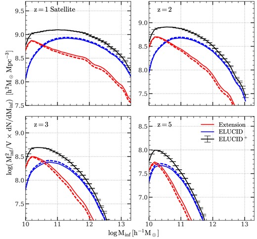
Infall mass functions of satellite subhalos in ELUCID. This figure is the same as Fig. 1, but for satellite subhalos selected at |$z$| = 1, 2, 3, and 5, respectively.
Fig. A2 shows the marginal distributions of satellite subhalos in the space of various properties at |$z$| = 2. Similar to the results of |$z$| = 0 shown in Fig. 5, subhalos simulated by ELUCID are significantly different from those by the reference simulation, TNGDark, in the one-dimensional marginal distributions of rlf, θr, lf, Minf, sat/Mhalo, host, and |$z$|inf, as well as in all the two-dimensional marginal distributions. This again indicates the incompleteness of the satellite population in ELUCID and that the incompleteness depends on subhalo properties. Distributions of the amended population in |$\rm ELUCID^{+}$| match almost perfectly those in TNGDark, as seen from a comparison between the results shown by the red and grey colours. The K-S statistics of the 1D marginal distributions between |$\rm ELUCID^{+}$| and TNGDark are all less than 0.1, indicating a good match. All these again verify the reliability and precision of our extension algorithm.
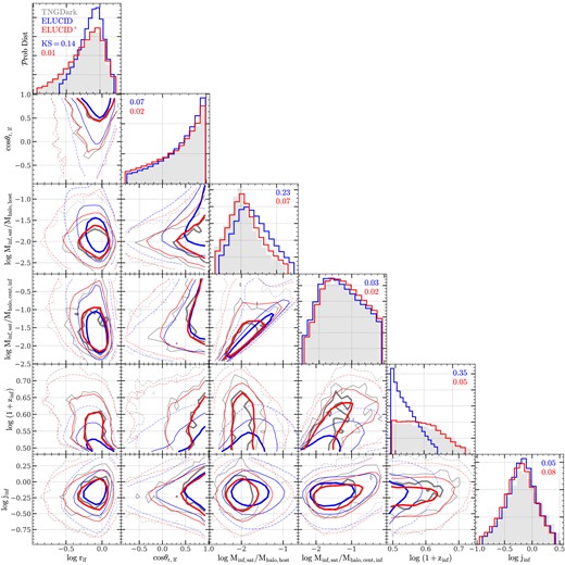
Marginal distributions of satellite subhalos in the projected spaces of properties as indicated by legends of individual axes. This figure is the same as Fig. 5, but for satellite subhalos at |$z$| = 2.
APPENDIX B: COMPLETENESS AND CONVERGENCE OF THE EXTENSION
As outlined in Section 3.1, the extension algorithm operates on branches of a target simulation S at low resolution, requiring that each branch includes at least one resolved central subhalo. The completeness of the extended trees is thus constrained by this requirement. On the other hand, to ensure applicability to all kinds of halos in S, the reference simulation S′ at high resolution must encompass a representative population of halos in terms of mass, environments, and assembly histories within the universe. The volume size of S′ must meet these requirements.
Prior to applying the extension algorithm to a specific target simulation, it is imperative to conduct tests that quantify the completeness of the output trees from S and verify the fulfillment of requirements for S′ in terms of desired summary statistics. In this appendix, we provide an example of such tests employing a pair of N-body simulations: |$S=\,$|TNG100-3-Dark (referred to as |$\rm TNGDark_{LR}$|) and S′ = TNGDark. |$\rm TNGDark_{\rm LR}$| serves as a low-resolution counterpart of TNGDark, sharing the same box size but possessing a lower mass resolution of |$m_{\rm dark\ matter}=3.84\times 10^8 \, h^{-1}\, {\rm M_\odot}$| comparable to that of ELUCID. The specific choices of variables and parameters are the same as those employed in Section 3.3. Given that these two simulations have identical cosmology and initial condition, we can assess the limitations and requirements of the extension algorithm itself, unaffected by discrepancies in cosmology and volume sampling.
B1 Completeness of the extended population
Fig. B1 shows the infall mass functions of satellite subhalos at four different redshifts, obtained from the target simulation S = TNGDarkLR using the same method as in Fig. 1. By comparing the extended population (grey lines) with the simulated one (blue lines), it is evident that the low-mass end of the mass function is significantly elevated at each redshift. However, when compared to the results obtained from the high-resolution simulation TNGDark (black lines), the extended mass functions are still lower by 0.05 (0.15) dex at |$z$| = 0 (|$z$| = 5). This incompleteness becomes apparent at infall masses of |$\sim 10^{11} \, h^{-1}\, {\rm M_\odot}$| and increases as the mass decreases to the 32-particle resolution limit of |${\rm 10^{10.1}} \, h^{-1}\, {\rm M_\odot}$|. This discrepancy arises directly from a limitation of the extension algorithm: it is unable to generate a branch when the entire central stage is unresolved by S. The extension algorithm should, therefore, be used with caution when these limitations are of critical importance to the application, particularly for subhalos with infall masses that approach the resolution limit of the target simulation. Alternatively, deep-learning-based superresolution techniques, such as those proposed by Li et al. (2021) and Ni et al. (2021), offer a potential solution to the problem of incompleteness in unresolved subhalos. None the less, it is important to note that such methods currently only apply to individual snapshots and are incapable of recovering assembly histories of unresolved subhalos. Thus, a potential solution is to perform these methods at a given snapshot of the low-resolution simulation, reaching the desired mass limit, statistically match the superresolved subhalos to those with well-resolved histories in a high-resolution simulation, and integrate these histories back into the low-resolution simulation. This approach needs further exploration. Above |$10^{11.5} \, h^{-1}\, {\rm M_\odot}$| (equivalent to ∼1000 particles), the extended mass functions are in good agreement with those derived from TNGDark at all redshifts. This indicates that unresolved branches do not affect the completeness of the extended population with mass above this threshold.
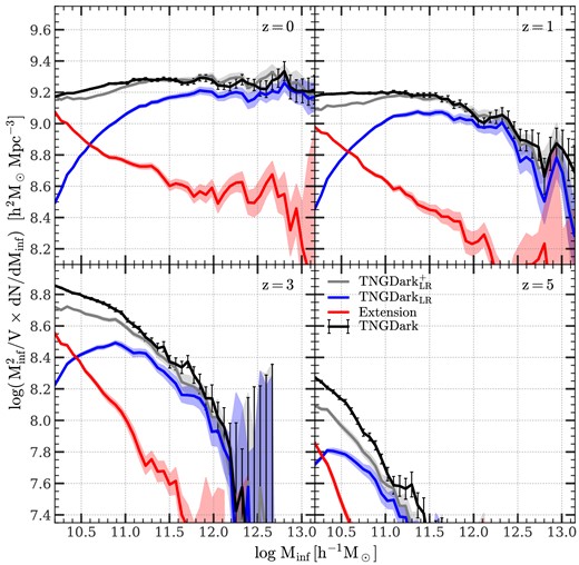
Infall mass functions of satellite subhalos in TNGDark (black line), |$\rm TNGDark_{\rm LR}$| (blue line), and the amended version, |$\rm TNGDark_{\rm LR}^+$| (grey line), at redshifts |$z$| = 0, 1, 3, and 5. The red lines in the graph indicate the subhalos created through the extension. All other details are consistent with what was presented in Fig. 1.
B2 Convergence of the algorithm
To determine the required volume size of the reference simulation, we apply the extension algorithm to |$\rm S= TNGDark_{\rm LR}$| with a series of subvolumes in |$\rm S^{\prime }=TNGDark$| of different sizes. These subboxes have side lengths of Lsub = 20, 25, 32, 40, 50, and |$60\, \, h^{-1}\, {\rm {Mpc}}$|, respectively. The obtained results for each subbox are compared to those of the full box with |$L_{\rm sub}=L_{\rm box}=75\, \, h^{-1}\, {\rm {Mpc}}$|. The chosen subboxes correspond to fractions |$f_{\rm sub} = 2$|, 4, 8, 15, 30, 51, and 81 per cent of the full volume. The infall mass functions of satellite subhalos at |$z$| = 0 are presented in Fig. B2, while the TPCFs of all subhalos, both central and satellite, in different mass bins are shown in Fig. B3.
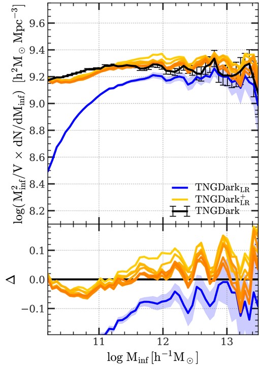
The same as Fig. B1 but here we show the infall mass functions of satellite subhalos at |$z$| = 0 extended using various subvolumes of the reference simulation. The results are represented by orange lines, from the lightest to darkest shade, corresponding to subvolumes of 2, 4, 8, 15, 30, 51, 81, and 100 per cent of the reference simulation’s volumes, respectively.
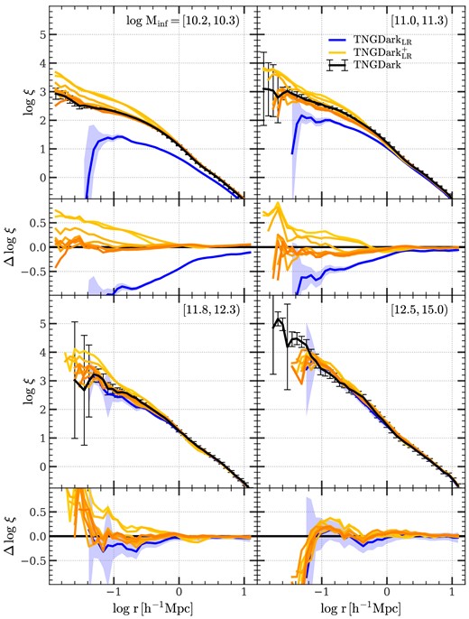
The same as Fig. B2, but here we show the TPCFs of all subhalos (central and satellite) at |$z$| = 0 in four different ranges of infall masses.
It is seen that the mass function of the extended population remains stable regardless of the volume size of the reference simulation. The difference in mass functions between the smallest subbox (|$f_{\rm sub}=2~{{\ \rm per\ cent}}$|) and the full box is less than 0.1 dex for |$M_{\rm inf} \lt 10^{12} \, h^{-1}\, {\rm M_\odot}$|, with the algorithm demonstrating convergence when |$f_{\rm sub} \ge 15~{{\ \rm per\ cent}}$|. However, for higher mass subhalos (|$M_{\rm inf} \geqslant 12 \, h^{-1}\, {\rm M_\odot}$|), fluctuations are more evident in both the mass functions themselves and the differences between them. This is due to the rarity of massive (sub)structures within a limited volume. Thus, for such massive subhalos, a larger subvolume of S′ yields a more unbiased result.
The analysis of the higher order statistic, TPCF, is more complex. When using a subbox with |$f_{\rm sub}=2~{{\ \rm per\ cent}}$|, the TPCF of the extended population significantly overestimates the clustering of subhalos of all masses at |$r \lt 0.5 \, h^{-1}\, {\rm {Mpc}}$|. This overestimation is more significant for lower mass subhalos and smaller halo-centric distances, where the extension algorithm needs to create more subhalos. As the subvolume of S′ increases, the TPCF of S becomes more similar to that of TNGDark and converges at |$f_{\rm sub} \ge 15~{{\ \rm per\ cent}}$|.
Based on these tests, we can conclude that for a target mass resolution comparable to |$\rm TNGDark_{LR}$| and the summary statistics considered here, a subvolume of |$L_{\rm sub} \sim 40\, h^{-1}\, {\rm {Mpc}}$| (approximately 15 per cent of the volume of TNGDark) is marginally sufficient for the algorithm to function properly. As a result, using TNGDark as the reference simulation is a reliable choice for extending ELUCID.
