


ABSTRACT
The early, active history of our Sun is still not fully understood. Observations of the magnetic fields on active young solar-type stars allow us an insight into the early evolution of our Sun. Here we present Doppler and Zeeman–Doppler images of the young late-F star HIP 71933 (HD 129181) at multiple epochs to add to the growing data about the evolution of magnetic cycles in solar-type stars. Spectroscopic data were obtained over seven epochs spanning 10 yr of observations, with two epochs including spectropolarimetric data. The brightness maps at all epochs show a consistent spot activity in a non-uniform ring at a latitude of approximately +60° with no polar spot present in any epoch. The two magnetic field maps taken ∼2 yr apart show a strong poloidal field configuration with most of the poloidal field energy in the dipolar configuration. The magnetic maps show no evidence of a polarity reversal. We were able to measure the differential rotation from one of the seven epochs using the brightness data finding a dΩ of 0.325 ± 0.01 rad d−1. The values for the rotational period and differential rotation found for HIP 71933 are consistent with values found for other late-F or early-G stars. The dominant poloidal features and the limited spots at the pole are unusual for a rapidly rotating star but not unique.
1 INTRODUCTION
The magnetic field of the Sun drives its activity cycles, the heating of its outer atmosphere and wind, and affects the Earth’s magnetosphere and biosphere (Babcock 1961; Glassmeier et al. 2009; Charbonneau 2014; Ragulskaya 2018). We need a solar dynamo theory that can produce an accurate model of how the Sun produces its magnetic field, as well as supporting a wider range of basic stellar parameters, such as mass and rotation rate (Ossendrijver 2003). To this end, it is useful to build a data base of the magnetic characteristics of other solar-type stars to help support this effort.
Spots on the surface of the Sun were first recorded in ancient times by Chinese astronomers as they can be seen by the naked eye (Temple 1988), while observations of sunspots via a telescope were first recorded by Thomas Harriet in the 17th century, despite credit usually given to Galileo for this discovery (Vokhmyanin, Arlt & Zolotova 2020). The association of these dark sunspots with magnetic flux lines erupting from the surface of the Sun was first made by George Ellory Hale in 1908 (Hale 1908). They have since been observed on other stars, usually through the photometric dimming of the stellar surface as these starspots rotate in and out of view. In 1983, a technique was developed, called Doppler imaging (DI) that provides a method to resolve the surface characteristics of a distant star by measuring the distortion that a dark spot creates on a spectral line (Vogt & Penrod 1983). Through DI it is now possible to map surface features on stars by observing deviations in a line profile caused by the passage of spots across the surface as the star rotates (Rice 2002). Through the extension of DI with the observation of not only the intensity of the stellar light but also its polarization, we are able to use Zeeman–Doppler imaging (ZDI) to now not only map the surface spot features but also the polarization of the magnetic field across the stellar surface (Semel 1989).
Since the 1990s a small number of telescopes around the world have had polarimeters attached to high-resolution spectrographs (i.e. a spectropolarimeter) to capture polarization of line profiles necessary to use ZDI to record the large-scale magnetic field structure of young solar-type stars. From these observations, we see that young solar-type stars often show persistent polar spots, large-scale azimuthal fields, a wide range of differential rotation rates, and global field changes among stars with multiple observations (Carter, Marsden & Waite 2015). However, this data is still limited by the small number of solar-type stars that have been observed thus far. This is particularly true for young late-F stars. F-type stars occupy a range of temperatures and masses where the boundary between convection-generated magnetic fields, which operate in cool stars, and fossil fields, found in a number of hot stars, may lie. Hotter stars with thin convection zones are not able to sustain a dynamo-driven magnetic field, while it is thought that all cooler stars, with thicker convection zones, have some sort of magnetic dynamo. Lying at this boundary F-stars occupy an important region of study (Landstreet 1991; Mestel 2012; Seach et al. 2020).
Currently the number of F-stars studied is low, particularly for young F-stars. For mature F-stars they have been found to host rather rapid magnetic cycles. Tau Bootis (F7V, ∼1 Gyr; Borsa et al. 2015) has ultrarapid magnetic cycle of ∼240 d (Mengel et al. 2016; Jeffers et al. 2018), while HD 75332 (F7V, ∼1.88 Gyr) also shows a rapid magnetic cycle of ∼1.06 yr (Takeda et al. 2007; Brown et al. 2021). For young F-stars the picture is less clear with no real cycles yet evidenced. The young late-F stars HR 1817 (F7V, ∼25 Myr; Mengel 2005), HD 35296 (F8V, ∼30–50 Myr; Waite et al. 2015), and V1358 Ori (F9V, ∼30 Myr; Zuckerman et al. 2011) all show complex magnetic fields with a mixture of poloidal and toroidal field (Mengel 2005; Marsden et al. 2006a; Waite et al. 2015; Hackman et al. 2016; Kriskovics et al. 2019), while also having polar spots, with the exception of V1358 Ori (Hackman et al. 2016) that does not so far show no evidence of magnetic cycles, although V1358 Ori is suspected of having a ∼1600 d cycle according to its photometric data (Kriskovics et al. 2019). Our objective is to add to this small observational data base on the evolution of surface magnetic structures on young late-F stars.
Waite et al. (2011) conducted spectroscopic and spectropolarimetric observations of a number of active stars to create a candidate list of solar-type stars for potential follow-up ZDI observations. HIP 71933 emerged from this list as a young reasonably bright (V = 8.5), rapidly rotating (v sini = 75 km s−1), and young (∼15 Myr) late-F star, which showed a magnetic field detection in the one spectropolarimetric observation published by Waite et al. For this reason HIP 71933 was chosen to be observed using both spectroscopy and spectropolarimetry, over several epochs with multiple telescopes, to look for any potential evolution of its surface features.
This is the second paper in a series studying multiple epochs of young solar-type stars and the evolution of their brightness and magnetic features. The first paper studied the young solar-type star HIP 89829 (G5V; Perugini et al. 2021, hereafter Paper I). Here we provide analysis of a young F8V star HIP 71933, reconstructing its surface brightness and magnetic field topology over a span of 10 yr. We present basic stellar parameters in Section 2. Section 3 describes the observation and reduction methodology. Section 4 provides results of this study and analysis is provided in Section 5.
2 HIP 71933 PARAMETERS
HIP 71933 is classified as an F8V star (Torres et al. 2006), with the fundamental parameters for this star listed in Table 1. Most of these parameters are obtained from the European Space Agency’s Gaia space mission, but several were obtained empirically in this study using the methods described in Section 3.2.
Fundamental parameters for HIP 71933 (HD 129181, Gaia DR2 5905397139423601792).
| Parameter | Value |
|---|---|
| Right ascensiona | 14h42m5s |
| Declinationa | −48°47′|$59{_{.}^{\prime\prime}}28$| |
| Distancea | 90.033 ± 0.04 pc |
| Luminositya | 2.839 ± 0.028 L⊙ |
| Radius (R)a | 1.60 ± 0.05 R⊙ |
| Massb | 1.3 ± 0.05 M⊙ |
| Ageb | 15 ± 2 Myr |
| Photospheric temperature (TP)a | 5922.1 ± 155 K |
| Spot temperature (TS)c | 4022 ± 200 K |
| Photosphere–spot differencec | 1900 ± 200 K |
| Classificationd | F8V |
| vsinie | 76|$^{+0.5}_{-0.2}$| km s−1 |
| Inclination anglee | 37° ± 10° |
| Rotational periode | 0.67 ± 0.05 d |
| Rotation rate at equator (Ω)e | 9.4635 ± 0.05 rad d−1 |
| Rotational shear (dΩ)e | 0.325 ± 0.01 rad d−1 |
The Gaia spacecraft has measured parallax, position, brightness, and surface temperature for approximately 1.7 billion stars by 2020 (Gaia Collaboration et al. 2021). For HIP 71933 the measured parallax of 11.107 ± 0.024 mas converts to a distance of 90.033 ± 0.04 pc. Luminosity was measured to be 2.839 ± 0.028 L⊙ and photospheric temperature to be 5922.1 ± 155 K (Gaia Collaboration et al. 2018). Using brightness models compared against DI observations, Berdyugina (2005) plotted the variation in starspot temperatures against photospheric temperatures of stars of different stellar classifications (see fig. 7 in Berdyugina 2005). This figure gives a photospheric–spot temperature difference of 1900 ± 200 K for the surface temperature of HIP 71933. We therefore estimate a spot temperature of 4022 ± 200 K.
Using the photospheric temperature and luminosity values obtained from the Gaia releases, we can place HIP 71933 on a grid of stellar atmospheric models determined by Baraffe et al. (2015); see Fig. 1. Here we estimate a mass of ∼1.3 ± 0.05 M⊙ and an age of ∼15 ± 2 Myr for HIP 71933. This is a slightly younger age than ∼20 Myr recorded by Waite et al. (2011) as we are using the more recent theoretical isochrones of Baraffe et al. (2015), along with the recent Gaia release (Gaia Collaboration et al. 2018).
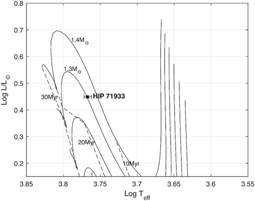
Evolutionary status of HIP 71933 with isochrones from the Baraffe et al. (2015) evolutionary models. The graph is a Hertzprung–Russell (HR) diagram with the solid lines representing pre-main-sequence (PMS) evolutionary tracks for stellar masses of 0.9–1.4 M⊙ in 0.1 M⊙ increments. The dashed lines are age isochrones for stellar ages of 10, 20, and 30 Myr. Luminosity and surface temperature and errors for HIP 71933 are taken from Gaia Collaboration et al. (2016, 2018). From this plot we estimate a mass of 1.3 ± 0.05 M⊙ and an age of 15 ± 2 Myr.
Values for vsini, radial velocity (RV), inclination, and rotational period were derived in this study by varying these parameters individually to achieve a minimum χ2, using the Stokes I data, as explained in Section 3.2. The vsini and rotational period derived in this study are 76 ± 0.5 km s−1 and 0.67 ± 0.05 d, respectively. This compares with a vsini value of 75 ± 1.0 km s−1 reported by Waite et al. (2011) and 75 km s−1 reported by Desidera et al. (2015). Desidera et al. (2015) also report a value for rotational period of 0.67 d, the same as our value. We derive a stellar inclination of ∼37° ± 10° that was the best χ2 of the selected epochs where the phase coverage was the best (see Fig. 2). The Gaia Data Release 2 (DR2) radius is given as 1.6 R⊙ (Gaia Collaboration et al. 2016). Using this along with our derived vsini of 76 km s−1 and a rotational period of 0.67 d, an inclination of |$38{_{.}^{\circ}}95$| can be calculated that is consistent with our modelled value.
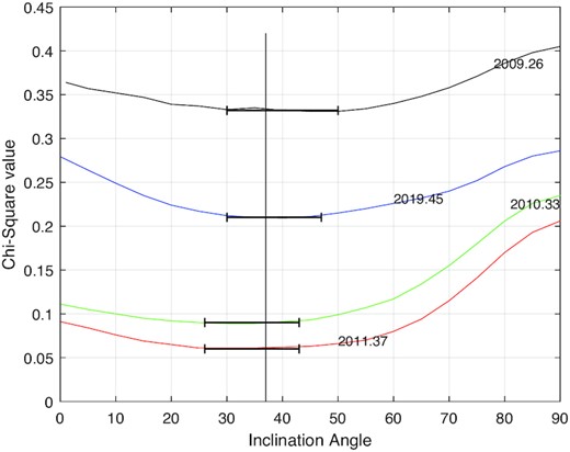
Inclination angle analysis. The inclination angle used in the DI process was varied by 1° increments for each epoch and the χ2 value determined. Epochs 2009.34, 2012.26, and 2018.07 were excluded from this plot because of less than optimal phase coverage. The graph shows the error in the inclination at the points where the inclination angle begins to change for higher χ2 values. This region is shown by the error bars. The average lowest χ2 value occurs ∼37°, shown by the vertical line. This value is consistent with an inclination calculated from the Gaia radius and our derived value for vsini as discussed in Section 2. Based upon the plots we estimate an error margin of ∼±10°.
RV values for HIP 71933 have been reported in previous studies. The Very Large Telescope (VLT)/NaCo large program (Desidera et al. 2015) reports an RV of 5.5 km s−1 and identifies HIP 71933 as a suspected spectroscopic binary (SB), however we note that there is no record of HIP 71933 (or HD 129181) in the Ninth Catalogue of Spectroscopic Binary Orbits (SBORBITCAT; Pourbaix et al. 2004). The Pulkovo compilation of radial velocities (Gontcharov 2006) reports a mean RV of 12.3 km s−1. Our study derives a variation in RV between epochs from 4.5 to 6.4 km s−1 (see Table 2 and Section 5.6). Since there is no data in our study before 2009 and none between 2013 and 2018, it is difficult to identify a period, however these values support the previous report of HIP 71933 being a suspected SB. See Section 5.6 for more detail.
Data derived from the DI analysis. Column 1 lists the observation epoch. Column 2 is the total number of Stokes I exposures for each epoch. Column 3 lists the signal-to-noise ratio (SNR) for each least-squares deconvolution (LSD) profile. Column 4 lists the percentage spot coverage for the entire stellar surface. Column 5 lists the RV for each epoch. Based upon a plot of RV values with decreasing χ2 values, we estimated an error of 0.1 km s−1 for the Anglo-Australian Telescope (AAT) and HARPSpol and 1.0 km s−1 for the 2.3-m telescope (see Section 5.6 for a discussion of this difference).
| Epoch | No. of exposures | LSD SNR | Spot percentage | RV values (km s−1) |
|---|---|---|---|---|
| 2009.26 | 31 | 937 | 1.80 | 5.7 ± 0.1 |
| 2009.34 | 18 | 541 | 0.73 | 5.9 ± 1.0 |
| 2010.33 | 45 | 832 | 1.47 | 6.1 ± 1.0 |
| 2011.37 | 70 | 1045 | 2.00 | 6.4 ± 0.1 |
| 2012.26 | 22 | 871 | 1.43 | 5.8 ± 1.0 |
| 2018.07 | 10 | 868 | 1.67 | 5.7 ± 1.0 |
| 2019.46 | 56 | 835 | 1.69 | 4.5 ± 1.0 |
3 HIP 71933 OBSERVATIONS
3.1 Observations overview
Three telescopes were used to obtain seven epochs of HIP 71933 observations over a period of 10 yr (see Table 3 for a summary). Epochs 2009.34, 2010.33, 2012.26, 2018.07, and 2019.46 were recorded using the Australian National University’s (ANU) 2.3-m telescope at the Siding Spring Observatory in New South Wales, Australia. This telescope is equipped with a high-resolution Échelle spectrograph with a resolution R ∼ 24 000. This spectrograph is attached to the Nasmyth focus of telescope and moves as the telescope tracks (see Burton 2013 for a description). Stokes I data only were recorded. From these intensity measurements DI mapping was used to calculate a spot distribution map of the star’s surface (see Fig. 3). A more detailed description of the DI process is described in Section 3.2.
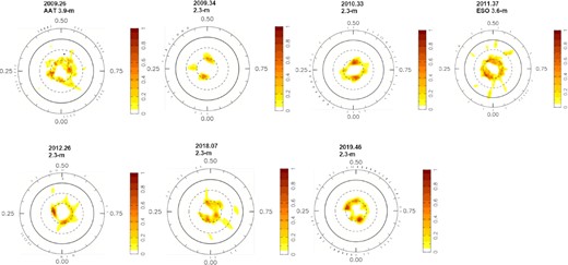
Maximum entropy brightness spot occupancy for all seven epochs. The images are flattened polar projections extending down to a latitude of −30°. The dashed lines are +30° and +60° latitudes and the bold line is the equator. The radial tics are the rotational phases at which HIP 71933 was observed. Note the absence of spots at the visible pole and the consistent ring of spot clusters at the +60° latitude. Spot filling varies from 1.6 per cent to 3.8 per cent.
Log of spectroscopic observations of HIP 71933 for our epochs. The first two columns list the epoch of the observation and telescope. Column 3 lists the instrument resolution. Columns 4, 5, and 6 list the date, start time, and end time for the exposures. Column 7 lists the number of usable exposures in the sequence. Column 7 lists the rotational cycles for each epoch from the first to last exposure. The zero phase was calculated to be the mid-point of the first epoch and is at JD 245 4932.2110 (see equation 1). The zero-points for all subsequent epochs are calculated as an integer number of rotations starting with the zero-point of the first epoch that is the closest to the mid-point of each epoch.
| Epoch | Telescope | Instrument resolution | Date | ut start | ut end | No. Stokes I exposures | Rotational cycle |
|---|---|---|---|---|---|---|---|
| 2009.26 | AAT | ∼70 000 | 2009 Apr 07 | 12:20 | 16:02 | 8 | −4.563 to 4.668 |
| 2009 Apr 08 | 11:01 | 16:45 | 12 | ||||
| 2009 Apr 09 | 11:40 | 18:22 | 7 | ||||
| 2009 Apr 13 | 16:11 | 16:55 | 4 | ||||
| 2009.34 | 2.3-m | ∼24 000 | 2009 May 04 | 12:39 | 17:36 | 7 | −1.214 to 2.070 |
| 2009 May 06 | 10:35 | 10:55 | 11 | ||||
| 2010.33 | 2.3-m | ∼24 000 | 2010 Apr 01 | 12:09 | 18:59 | 15 | −2.722 to 2.093 |
| 2010 Apr 02 | 12:38 | 19:13 | 11 | ||||
| 2010 Apr 03 | 13:05 | 17:16 | 10 | ||||
| 2010 Apr 04 | 12:22 | 17:20 | 9 | ||||
| 2011.37 | 3.6-m | ∼115 000 | 2011 May 16 | 02:04 | 23:20 | 12 | −3.384 to 4.147 |
| 2011 May 17 | 01:39 | 23:19 | 12 | ||||
| 2011 May 18 | 00:26 | 23:57 | 16 | ||||
| 2011 May 19 | 01:17 | 07:31 | 8 | ||||
| 2011 May 20 | 00:01 | 23:28 | 22 | ||||
| 2012.26 | 2.3-m | ∼24 000 | 2012 Apr 04 | 12:28 | 16:59 | 5 | −4.180 to 3.596 |
| 2012 Apr 05 | 15:11 | 18:44 | 3 | ||||
| 2012 Apr 06 | 16:29 | 17:30 | 2 | ||||
| 2012 Apr 07 | 11:15 | 17:41 | 6 | ||||
| 2012 Apr 09 | 11:51 | 17:41 | 6 | ||||
| 2018.07 | 2.3-m | ∼24 000 | 2018 Jan 25 | 16:45 | 18:37 | 4 | −2.763 to 1.794 |
| 2018 Jan 28 | 15:16 | 18:06 | 6 | ||||
| 2019.46 | 2.3-m | ∼24 000 | 2019 June 17 | 08:07 | 11:46 | 10 | −2.080 to 2.874 |
| 2019 June 18 | 08:04 | 12:16 | 12 | ||||
| 2019 June 19 | 08:05 | 16:06 | 16 | ||||
| 2019 June 20 | 08:02 | 16:02 | 18 |
For the Stokes V polarization data, we recorded two epochs at telescopes equipped with spectropolarimeters. Epoch 2009.26 was recorded at the 3.9-m Anglo-Australian Telescope (AAT) at the Siding Spring Observatory using the SEMPOL/University College London Spectrograph (UCLES) spectropolarimeter. The UCLES (now decommissioned) was a high-resolution èchelle spectrograph attached to the AAT. A spectropolarimeter was created by coupling a visiting polarimeter instrument called SEMPOL, named after the late Meir Semel (Semel 1989), with the UCLES spectrograph. This combination had a resolution of R ∼ 70 000. SEMPOL was positioned at the Cassegrain focus of the AAT and split the original signal into two beams of opposite circular polarization that fed into the UCLES spectrograph. Further information about the configuration of the SEMPOL polarimeter with the UCLES spectrograph is in Semel (1989), Donati et al. (2003), and Henrichs et al. (2012).
Epoch 2011.37 was recorded at the European Southern Observatory’s (ESO) La Silla Observatory near Santiago, Chile using the HARPSpol spectropolarimeter. The High-Accuracy Radial Velocity Planetary Searcher (HARPS) has been in operation since 2003 on the 3.6-m telescope at La Silla. It has a resolution of R ∼ 115 000 (Mayor et al. 2003). It also includes a demountable polarimeter that, like SEMPOL at the AAT, feeds two beams of opposite circularly polarized light by using wave plates to provide circular polarimetry data to the spectrograph (Snik et al. 2011). This configuration is referred to as HARPSpol. These later two observations (AAT and HARPSpol) provided us with the Stokes V data necessary to construct a topological magnetic field map of HIP 71933.
3.2 Observation and data reduction methodology
Prior to performing the DI and ZDI there are preparatory steps required to reduce the recorded data. We used the same technique as outlined in Paper I where more details on the reduction can be found. After the reduction, the extracted spectra are corrected for instrumental errors caused by small changes in atmospheric temperature and pressure. This was done with a line mask for an F8 star created from the atlas9 Kurucz atomic data base (Kurucz & Bell 1995). The heliocentric velocity of the Earth is then subtracted to correct the measured RV of the star. Finally, we ‘average’ the thousands of spectral lines from each exposure to increase the signal-to-noise ratio (SNR) using the technique of least-squares deconvolution (LSD; Semel 1989; Donati et al. 1997). A detailed review of this technique is provided in Kochukhov, Makaganiuk & Piskunov (2010). All of the above steps are organized into a pipeline with a single software package esprit (Echelle Spectra Reduction: an Interactive Tool; Donati et al. 1997).
We used previously developed maximum entropy codes developed by Donati & Brown (1997) to create brightness maps of the surface of HIP 71933 from the Stokes I data for each epoch. This code uses a maximum entropy regulating function defined by the algorithm developed by Skilling & Bryan (1984). Magnetic maps from the Stokes V data were created using mapping codes developed by Donati & Brown (1997). We used a weighting scheme favouring low |$\it l$| values that favour simpler magnetic fields consistent with previous research we are comparing to such as Marsden et al. (2011a) and Paper I. The rotational phase for each epoch was calculated by starting with the mid-point of the first epoch (2009.26). The starting point for each subsequent epoch was calculated by taking an integer number of rotations from the initial start point up to the closest centre of each data set. The determination of the starting point of each epoch using these steps enables us to somewhat match the phases between maps, however the error in the rotational period derived by our study will cause some shift in the phases. The rotational phase was computed using the ephemeris:
where JD is the observational date and ϕ is the rotational phase.
4 RESULTS
4.1 Stokes I and Stokes V image reconstruction
Using the LSD profiles we created surface brightness maps for all epochs and magnetic topology maps for two epochs (2009.26 and 2011.37). The results of the DI including spot coverage as a percentage of the stellar surface and RV values are listed in Table 2. There is a change in RV for each epoch with a difference of almost 2 km s−1 across the entire observation period. Polar projections of the surface brightness for each epoch are shown in Fig. 3. These figures show a distinctive ring at +60° latitude and a lack of spots at the visible pole throughout all epochs.
Table 4 shows the values for the magnetic quantities derived from the two magnetic maps, with magnetic energies given as percentages of the poloidal and toroidal components. Variations are obtained by increasing and decreasing vsini by +0.5 and −0.2 km s−1, inclination angle by ±10°, and differential rotation by one standard deviation.
Magnetic quantities derived from maps in Figs 4 and 5. Magnetic energies are shown as percentages of the poloidal and toroidal components. These values are separated into |$\it l$| values of 1, 2, 3, and ≥4, respectively. The last two values show the percentage values of the poloidal and toroidal field that are axisymmetric (m = 0). Variations were obtained by increasing and decreasing vsini by +0.5 and −0.2 km s−1, inclination angle by 10°, and differential rotation by one standard deviation (see Section 5.2).
| Quantity (per cent energy) | Epoch 2009.26 | Epoch 2011.37 |
|---|---|---|
| Total poloidal | 94|$^{+1}_{-0}$| | 83|$^{+2}_{-3}$| |
| Total toroidal | 6|$^{+0}_{-1}$| | 17|$^{+3}_{-1}$| |
| Poloidal (|$\it l$| = 1) | 62|$^{+2}_{-2}$| | 50|$^{+5}_{-1}$| |
| Poloidal (|$\it l$| = 2) | 14|$^{+2}_{-1}$| | 12|$^{+1}_{-1}$| |
| Poloidal (|$\it l$| = 3) | 7|$^{+1}_{-0}$| | 5|$^{+1}_{-1}$| |
| Poloidal (|$\it l$| ≥ 4) | 12|$^{+1}_{-1}$| | 14|$^{+2}_{-2}$| |
| Toroidal (|$\it l$| = 1) | 2|$^{+0}_{-0}$| | 5|$^{+1}_{-1}$| |
| Toroidal (|$\it l$| = 2) | 1|$^{+0}_{-0}$| | 2|$^{+1}_{-0}$| |
| Toroidal (|$\it l$| = 3) | 0|$^{+0}_{-0}$| | 1|$^{+1}_{-0}$| |
| Toroidal (|$\it l$| ≥ 4) | 3|$^{+0}_{-0}$| | 10|$^{+2}_{-2}$| |
| Axisymmetry poloidal | 82|$^{+3}_{-1}$| | 75|$^{+3}_{-1}$| |
| Axisymmetry toroidal | 5|$^{+0}_{-1}$| | 2|$^{+2}_{-2}$| |
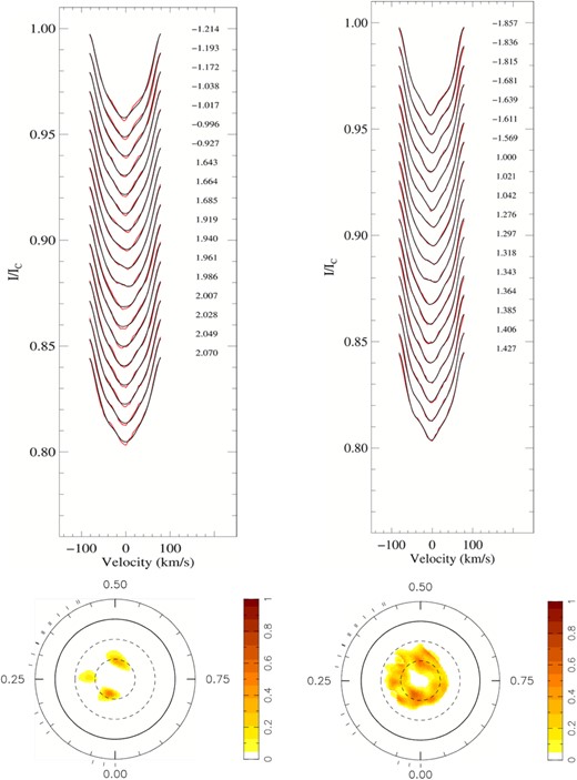
Figs 4 and 5 show the magnetic maps for epochs 2009.36 and 2011.37, respectively. The brightness map is shown again in the top left for comparison. The +60° ring is visible in the azimuthal magnetic field and both magnetic maps are predominately dipolar with the greatest strength in the poloidal field.
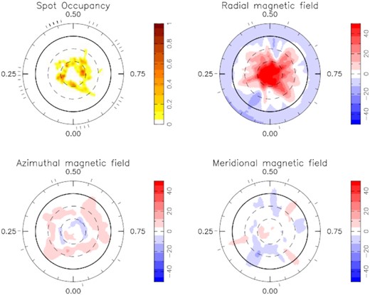
Maximum entropy brightness and magnetic image reconstructions for Epoch 2009.26. The spot occupancy (brightness) maps are the same as in Fig. 3. The scale bar for the magnetic maps provides field strength in Gauss (G) and polarity. We see a strong radial field at the visible pole and a weaker meridional near the equator. The azimuthal field shows the ring at the +60° latitude. The spot map in the upper left shows a 2.2 per cent coverage. Total global magnetic field strength is 12.3 G.
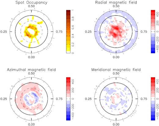
Maximum entropy brightness and magnetic image reconstructions for Epoch 2011.37. The spot occupancy map is the same as in Fig. 3. As in Fig. 4 the scale bar for the magnetic maps provides field strength in Gauss (G). Compared to Epoch 2009.26 (Fig. 4) we also see a strong radial field at the visible pole and a more defined ring at the +60° latitude in the azimuthal map. The spot map in the upper left shows a 4.0 per cent coverage. Total global magnetic field strength is 80.4 G.
Maximum entropy Stokes I intensity fits to the observed LSD profiles are shown in Figs A1–A5. Fig. A6 shows the fits to the Stokes V LSD profiles for the two epochs with magnetic data.
4.2 Differential rotation
The surface differential rotation of a star can be measured from the DI brightness images and ZDI magnetic maps taken during an individual epoch to determine the amount of rotational shear as seen from the star’s equator to pole. A solar-like differential law is incorporated into the imaging:
where Ω(θ) is the rotation rate at latitude θ in rad d−1, Ωeq is the equatorial rotation rate in rad d−1, and dΩ is the rotational shear between the equator and the poles (the differential rotation in rad d−1).
Each value of Ωeq and dΩ is treated as an independent pair and a map created for each pair. The resulting plot displays a range of χ2 values with better fits shown in darker colours, see Fig. 6. This technique is described in Petit, Donati & Collier Cameron (2002). Further error estimations were derived by varying the inclination by ±10°, vsini by +0.5 and −0.2 km s−1, and maximum entropy spot aim by ±5 per cent. These values are shown as crosses in Fig. 6.
In order to produce a well-defined paraboloid, spots should be visible from equator to pole of the visible hemisphere, with a number of observations evenly spaced through rotational phases and a resolution high enough to reveal shifts in spot movement. Of the seven epochs in this study, we were able to derive differential rotational parameters only from the Epoch 2011.37 DI observations using the HARPSpol spectropolarimeter. Differential rotation calculations using Stokes V for the two available epochs did not converge to definite values for rotation and shear. The value obtained for dΩ from Fig. 6 is 0.325 ± 0.01 rad d−1 and is listed in Table 1. This value of differential rotations was included in the DI and ZDI maps for all epochs.
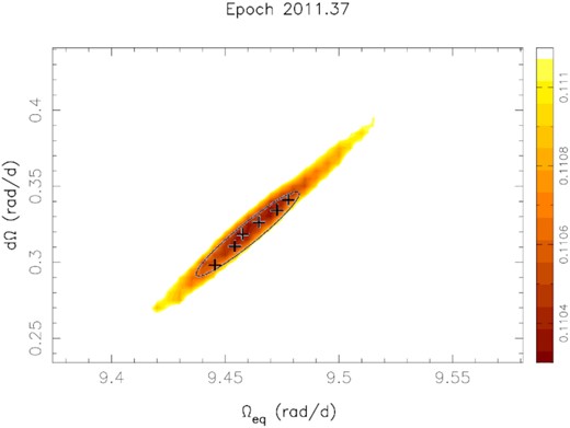
Differential rotation measurement for 2011 May (Epoch 2011.37) using Stokes I data. Values of dΩ are plotted against Ωeq. These values form a paraboloid (yellow-brown area of the plot, plotted to 3σ) with the best χ2 having the darkest value at the centre. The crosses on the graph are 1σ variances generated by changing the star’s inclination by ±10°, vsini by |$^{+0.5}_{-0.2}$| km s−1 and the maximum entropy spots aim by ±5 per cent. An ellipse is then drawn that contains all these values.
5 DISCUSSION AND ANALYSIS
5.1 Differential rotation
Using the parameters for HIP 71933 in Table 1 and the Baraffe et al. (2015) evolutionary models, we calculate a convective layer depth of 26 per cent of the stellar radius. Fig. 7 shows differential shear versus depth of the convective zone of several solar-type stars. HIP 71933 shows a differential shear at the higher end of these stars, especially HIP 89829 that exhibits a near solid body rotation. This is also in contrast with the findings of Reiners & Schmitt (2003) who report diminished differential rotation for rapidly rotating early F-type stars with vsini > 50 km s−1, although these stars are primarily mature stars.
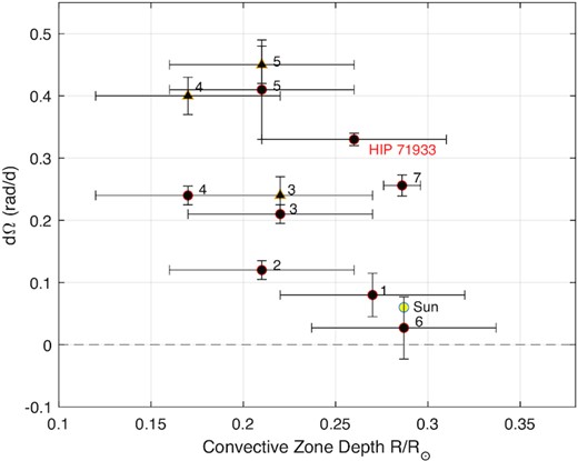
Surface differential shear dΩ versus convective zone depth as a function of solar radius for several solar-type stars. Dots show surface differential shear from surface brightness analysis and triangles from surface magnetic analysis. The convective zone depth was calculated from Siess & Forestini (2000) except for HIP 89829 (from Paper I), HR 1817 (Mengel 2005), and HIP 71933 (this paper) that used newer evolutionary models (Baraffe et al. 2015). This plot was taken from Marsden et al. (2011b) and updated with the last three stars. 1 – R58 (HD 307938), G2V (Marsden et al. 2005); 2 – LQ Lup, G8IV (Donati et al. 2000); 3 – HD 106506, G1V (Waite et al. 2011); 4 – HD 141943, G2 (Marsden et al. 2011b); 5 – HD 171488, G0V (Jeffers & Donati 2008; Marsden et al. 2011b); 6 – HIP 89829, G5V (Paper I); 7 – HR 1817, F8V (Mengel 2005).
It has been observed for some time that the surface temperature of a star directly affects the depth of its convective zone with hotter stars having thin or no convection zones and the coolest stars with convective zone depths down to the star’s centre (Böhm-Vitense 1992). F-type stars appear to occupy a special position on the Hertzprung–Russell (HR) diagram where the transition between these two states occurs at or earlier than F5 (Simon & Landsman 1991; Wolff & Simon 1997; Mizusawa et al. 2012; Seach et al. 2020). An examination of the data base of 135 stars recorded by Reiners & Schmitt (2003) shows that nine are later than F5-type stars and the remaining are earlier stars, including two A9-type stars. Hotter stars than F5 with thinner convective zones can be expected to exhibit less rotational shear. Late-F stars such as HIP 71933 should then be expected to be observed with deeper convection zones and higher rotational shear.
5.2 Stokes V magnetic map analysis
The magnetic maps from both the Epochs 2009.26 and 2011.37 show similar structure displaying a dominant dipolar field. The radial field shows a strong positive polarity at the visible pole and opposite polarity at the equator and possibly towards the opposite pole. It covers the entire pole in the Epoch 2009.26, but a ring can be seen in the same area in the maps of Epoch 2011.37. This may be due to the higher resolution available in the HARPSpol data (see Figs 4 and 5).
In both epochs there is an azimuthal ring at approximately +60° latitude around the visible pole with at least two and possibly three rings of alternating polarity in the visible hemisphere. The +60° azimuthal ring appears to be aligned with the ring of spots (see Fig. 3).
The poloidal field for HIP 71933 is dominant in both epochs (94 per cent for Epoch 2009.26 and 83 per cent for Epoch 2011.37). This is in contrast to previous research of solar analogues that infer the toroidal field component should become dominant for rotation periods of less than approximately 12 d (Petit et al. 2008). However subsequent to this early research dominant poloidal fields have been seen in other solar-type stars. Waite et al. (2015) report a dominant poloidal field (75 per cent) in 2009 for HD 29615. Hackman et al. (2016) report a similar percentage (62.8 per cent) for a 2013 observation of the same star, but with a reversed polarity, indicating that HD 29615 underwent a polarity reversal from 2009 to 2013. Waite et al. (2017) show a change in EK Draconis (HD 129333) from a dominant toroidal (83 per cent) in 2006 to a more balanced poloidal–toroidal in 2012 (57 per cent toroidal). Paper I also shows a dominant poloidal field for HIP 89829 in two epochs but again with a lower percentage (77 per cent in 2010 to 62 per cent in 2011).
The poloidal fields observed in the two epochs we have for HIP 71933 are at a higher percentage (82 per cent and 75 per cent) than any of the previous studies of other similar stars. These results show that rapidly rotating stars like HIP 71933 can have dominant poloidal magnetic fields, at least at some epochs.
The field strengths recovered in the Epoch 2011.37 are much higher than those recovered for the Epoch 2009.26 (see Figs 4 and 5). Previous studies of young solar-like stars report a decrease in the differences between the poloidal and toroidal field strengths during periods that may be magnetic field migrations (Hackman et al. 2016; Waite et al. 2017). Whereas we do see a small change in the dominance of the poloidal field on HIP 71933 between two epochs, this is not enough to account for large differences in the magnetic field maps. The field strength obtained from the ZDI process is related to the quality of the fit of the data so the additional resolution and quality of the HARPSpol spectropolarimeter is suspected to have allowed more of the magnetic field to be recovered for Epoch 2011.37. We do see a higher LSD SNR from this epoch (see Table 3). For these reasons we believe that the change in magnetic field strength seen in Figs 4 and 5 is likely instrumental due to the better quality of the HARPSpol data. We thus concentrate on the distribution and the percentages of the magnetic field properties we are comparing between the two epochs.
We know that our Sun has a dominant poloidal field during solar minimums at which time the internal toroidal field is at a maximum (Munoz-Jaramillo et al. 2008). The stability of the magnetic field components from our two magnetic observations of HIP 71933, the dominance of the poloidal field strength and the lack of evolution in the latitude of the spots seen in the brightness images may indicate that we may have observed this star during a low-activity cycle. This might also be supported by the stability of the ring-like structure in the brightness maps throughout the entire 10 yr observing period.
5.3 Spots and latitude distribution
As was done in Paper I, we display latitudinal distribution of spots in terms of fractional spottedness per the equation:
where S(θ) is the average spot occupancy at a given latitude θ and dθ is the width of each latitude ring. This is graphically shown in Fig. 8.
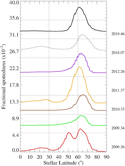
Fractional spottedness by latitude for all seven epochs. Fractional spottedness is based on the average spot occupance at each latitude and is defined by equation (3). Each epoch is shifted up by 0.044 for graphing purposes. The additional bump at +50° latitude seen at Epoch 2009.26 may indicate the end of a more active cycle as it appears only in the first epoch of the 10 yr of observations.
On HIP 71933 we see a ring-like structure at approximately +60° latitude consistent with the azimuthal ring seen in the magnetic maps. This structure is seen on the brightness maps in each epoch. The ring is confined mostly to the +60° latitude except for Epoch 2009.26 where additional spottedness can be seen between +40° and +60° latitude (see Figs 4 and 8). This might be explained by the additional resolution of the AAT versus the 2.3-m telescope, and we would expect to see similar additional spots at Epoch 2011.36 with HARPSPol. There is recovery of additional spotting at lower latitudes in this epoch, but not as much between +40° and +60° latitude. These additional features recovered between these latitudes in Epoch 2009.26 might be related to the spot evolution on HIP 71933 as they are seen only in the first epoch of the 10 yr observation time span and could potentially indicate the end of a more active phase of the star.
The darker spots seen in the +60° ring in the brightness maps are not as well defined in the magnetic maps for Epochs 2009.26 and 2011.37 (see Figs 4 and 5), but the spot ring appears to be aligned with the ring of azimuthal field on the stellar surface. Magnetic signatures from ZDI are produced by recovering the circularly polarized light from the stellar surface. This light is a very small percentage of the unpolarized light, and in the vicinity of dark spots will be smaller resulting in poorer recovery of the Stokes V signature (Donati et al. 1992, 1997).
The number of spot clumps and their location within the ring varies between epochs. This could be due to the number and distribution of observation phases, data quality, or spots forming and reforming on a continuous basis, however these spots do not display any major shift in latitude. Because of the low spatial resolution of DI maps, we cannot be certain if these clumps are a single spot or a group of smaller spots (Solanki & Unruh 2004; Isik, Schüssler & Solanki 2007). The long-term nature of this ring would seem to be consistent with the existence of long-term polar spots on many young solar-type stars, but in contrast with our understanding that spot evolution on rapidly rotating stars occurs in periods of weeks or months (Barnes et al. 1998; Paper I; Şenavcı et al. 2021). The persistence of the ring could mean that it is being formed by new spots added to the ring as others decay.
5.4 The effects of instrumental resolution and phase coverage
The visibility of spots on a star’s surface relative to our line of sight depends upon the latitude of the spot and the inclination of the star. The overall quality of the ability of DI to recover these surface features then depends upon the instrumental resolution of the spectrograph, the SNR, the vsini of the star, and the overall rotational phase coverage of the observing epoch.
In order to provide a complete image of a star, a minimum number of spectral profiles are needed that are evenly distributed in a rotational phase around the star. At least 8–10 observations spread evenly over the rotational phase space are needed to provide an accurate image (Vogt, Penrod & Hatzes 1987). Resolution and intensity of spot features, particularly at lower latitudes, are not as well recovered if the phase coverage of the observations is poor. This does not apply as much to higher latitude features with a high stellar inclination where spot features will always be visible. For stars with high inclination poor phase coverage can degrade the recovery of low-latitude spot features and radial and meridional magnetic field vectors (Donati & Brown 1997).
Concerning aperture size, instrumental resolution, and stability, there are significant differences between epochs of our observations of HIP 71933. Aperture size and instrumental quality is the best for the ESO 3.6-m HARPSPol (Epoch 2011.37) and the AAT (Epoch 2009.26), and we see superior spot recovery for these observations. We note that Epoch 2019.46 has the best phase coverage and we continue to see little or no low-latitude features. We have less than optimal phase coverage for Epochs 2009.34, 2012.26, and 2019.07, the poorest for Epoch 2009.34 (see Fig. 3). For this reason, we have eliminated these observations for the determination of stellar inclination (see Fig. 2). The poorest phase coverage is in Epoch 2009.34, which might contribute to its outlier vsini fit (see discussion in Section 5.5).
5.5 High-latitude features
As stated in Section 5.3 for HIP 71933 there is a consistent high-latitude ring at the +60° latitude. These high-latitude features are seen in both the brightness maps and magnetic maps. In contrast, there is an absence of evidence for spots in the polar regions.
Marsden et al. (2005) reported a potentially similar phenomena from DI observations of R58. R58 (HD 307938) is a solar-analogue G2V star with mass of 1.15 M⊙ and a radius of 1.18 R⊙. It has an age of 35 Myr, close to HIP 71933. A dip was displayed in the middle of most of the LSD profiles. This dip was believed to be caused by reflected moonlight scattered into the spectrograph as the observations were made during a full Moon. The dips appeared in the centre of the LSD profiles because of the similarities between the RV of the star and the terrestrial velocity toward it. The location of the dips interfered with the recovery of the spot distribution at the pole, leaving an absences of spots above the +60° ring in the brightness maps.
We reviewed the position and phase of the Moon during each of the epochs recorded for HIP 71933 using an ephemeris (Espenak 1999; Peat 2022). There was an average of 46° between the Moon and the star among all epochs. During Epoch 2010.33 the Moon was closest to HIP 71933 and during Epoch 2018.07 it was below the horizon. We did not include observations during cloudy nights and we do not see any of the dips reported by Marsden et al. (2005). We see only small dips in Epoch 2009.34 (see Fig. A2). During this observation the Moon was setting or below the horizon. We therefore discount solar contamination as the source of the lack of spotting at the pole.
These additional structure (dips) seen in the Epoch 2009.34 can be eliminated by inserting a vsini value of 74 km s−1, which results in a superior fit. This produces additional spottedness above the +60° latitude, however an absence of spots is still present at the pole (see Fig. A2). This vsini value does not provide the best fit for other epochs, all of which produce a minimum χ2 at a vsini of 76 km s−1. Brightness maps for all epochs show additional spotting above +60° with lower values of vsini, however this results in an unreliable statistical fit (Skilling & Bryan 1984). The only vsini that produces a viable maximum entropy fit for all observations is a value of 76 km s−1. Since the vsini should not vary, the singular value needed for the best fit for Epoch 2009.34 may be due to poorer stability of the spectrograph on the 2.3-m telescope and the lack of phase coverage for this epoch.
Unlike HIP 71933, the spot distribution observed on other young solar-type stars almost always shows a polar spot. A large polar spot was suspected from observations of EK Draconis (G1.5V) in 1996/1997 based upon spectral line inversion (Strassmeier & Rice 1998). Later observations of EK Draconis using DI show a large polar spot along with weaker lower latitude features (Şenavcı et al. 2021). Other examples are HD 307938 (R58, a G2V star; Marsden et al. 2005), HR 1817 (F8V; Marsden 2018), V530Per (G8V; Cang et al. 2021), HD 199178 (G5IV; Hackman et al. 2019), and HIP 89829 (G5V; Paper I). In some cases the polar spot can be slightly decentred as seen on He 699 (a G dwarf; Jeffers, Barnes & Collier Cameron 2002). Whether these areas consist of large individual spots or groups of smaller spots is not certain because of the lack of resolution currently available with DI (Willamo et al. 2019). The persistent presence of large polar spots on young solar-type stars may be due to a Coriolis effect pushing spots to higher latitudes due to the star’s rapid rotation, or may be forming at lower latitudes and move poleward due to subsurface meridional flows (Waite et al. 2011).
In the early days of DI, the presence of excessive polar spots was attributed to observed inversions or ‘flat bottoms’ of the profiles of the stars. The large polar spots observed were thus believed to be computational artefacts (Kürster, Schmitt & Cutispoto 1994; Rice 2002). Subsequent observations of other stars by different groups using differing techniques have provided compelling evidence that polar spots do exist and are common on rapidly rotating stars (Carter et al. 2015; Choudhuri 2017).
Azimuthal ring-like structures at high latitudes have been reported on other young solar-like stars with some degree of persistence. A high-latitude azimuthal ring almost completely circling the visible pole on AB Doradus (a K0 dwarf star) is reported by Donati & Cameron (1997) and again seen 2 yr later by Donati et al. (1999). Marsden et al. (2006b) and Alvarado-Gómez et al. (2015) reported a ring-like azimuthal structure on HD 1237 (a G8V star), although closer to mid-latitude (+45°), and reported an azimuthal field around the rotational axis of HD 171488 (a G0V dwarf star) with a strong latitude dependence that is independently reported by Jeffers & Donati (2008) and Jeffers et al. (2011).
Several numerical simulations have tested dynamo models that create wreath-like structures on surfaces of solar-type stars that are rotating faster than the Sun. Schrijver & Title (2001) proposed a random walk model of flux dispersal that produces a ring-like structure at high latitudes surrounding a polar spot at opposite polarity. Granzer et al. (2000) propose a similar appearance of spots for stars between 1.0 and 1.7 M⊙ and rotation rates approximately 50 Ω⊙. Their model is based upon the idea that rapid stellar rotation causes starspots to shift towards the poles (Schüussler & Solanki 1992) and that high-latitude structures are dependent upon the ratio of the young star’s small core size to the size of its radiative zone. However, in both papers a polar spot is predicted, in contrast to what we see in HIP 71933.
Holzwarth & Schüssler (2002) conducted a series of simulations of starspots for binary systems with two solar-type components, using existing flux tube approximation numerical codes. They find that preferred longitudes for spot clusters can be caused by tidal effects from a secondary on the flux tubes that erupt and create clusters of starspots. If the flux tubes originate in the convection zone and take several months to erupt, there is a cumulation of tidal effects occurring more often in fast rotating stars. These eruptions tend to occur in clusters about 180° apart, with the clusters seen in a wreath at high latitudes (Holzwarth 2004). In these simulations the flux tubes originate at the base of the convection zone.
Our observations of HIP 71933 do meet the mass criteria of Schrijver & Title (2001) (1.0–1.7 M⊙) and are at the high end of the rotation rates simulated (from 3 to 50 Ω⊙). We do see large spots forming roughly 180° apart in Epochs 2009.34 and 2010.33. Epochs 2012.26 and 2019.46 however show clusters that are not exactly opposite with additional spot clusters in between them (see Fig. 3). These could be spot groups that are moving around under the influence of the star’s differential rotation. The ring on HIP 71933 is azimuthal and highly axisymmetric, but differs from the simulations in that we do not see a strong spot feature at the visible pole.
The rapidly rotating K dwarf HD 197890 (Speedy Mic) was observed in 1989 using DI without a polar spot. Referencing previous observations of AB Doradus, the authors thought this might be a consequence of activity cycle and point out that a flat bottom profile that is indicative of a strong polar spot is not present in their LSD profiles (Barnes et al. 2001).
HIP 71933 shows a consistent lack of polar spots over a time span of 10 yr. Our LSD profiles also do not exhibit the flat-bottom profile associated with a strong polar spot. We have a 6 yr gap in the observations between 2012 and 2018 however the brightness maps remain similar on either side of this gap. We see this feature in data from three different telescopes and spectrographs. While we cannot rule out that the lack of polar spots at the visible pole may be an artefact of the observational set-up and analysis, the internal consistency of our results over all instruments and the fact that other stars taken with the same instruments (i.e. Paper I; Marsden et al. 2005; Mengel 2005; Waite et al. 2011) do not show such obvious lack of polar spots, suggests that it is more likely that HIP 71933 lacked obvious polar features at the times observed. Thus HIP 71933 appears to be an unusual rapidly rotating star without a polar spot.
5.6 Active latitudes, radial velocity measurements, and the possibility of a companion
Fig. 9 plots the RV values we recorded in this study versus time. These values show what might be a portion of a cycle between 2008 and 2012, but are separated by too much time to identify a close-orbiting companion, and we do not have enough data to identify a longer period RV signature. RV values of single digit km s−1 and hundreds of m s−1 have been observed for stars that are known visual binaries (Katoh, Itoh & Sato 2018). Sonbas et al. (2022) record RV measurements for a known hot Jupiter (HJ) orbiting HAT-P-36 (a G-type star) at 400 m s−1. Our recorded RV values for HIP 71933 might support the existence of a large-mass exoplanet but would seem more likely a small stellar companion, if a companion exists.
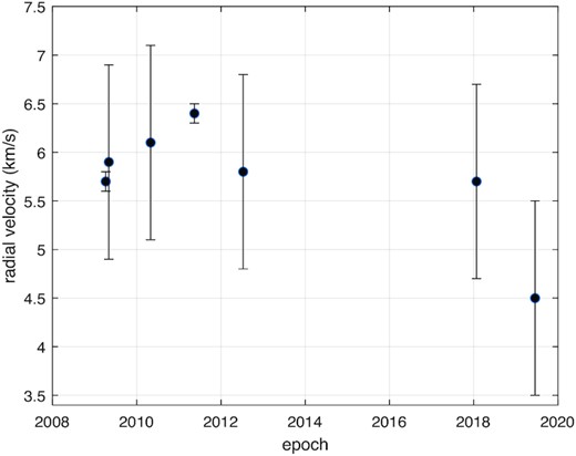
Radial velocity (RV) values plotted over time for all epochs. Error bars were estimated by examining the RV values derived with decreasing χ2. RV errors for Epochs 2009.26 and 2011.37 are the smallest due to the superior resolution and stability of the spectroscopic measurements made at the AAT 3.9-m telescope and the ESO 3.6-m telescope. There is no data between 2013 and 2018.
If HIP 71933 is a binary system as some previous studies have suggested, then we might see evidence of a secondary in the LSD profiles. Secondary stars can be seen in LSD profiles provided the velocity space is wide enough and the LSD signature is sufficiently large (Marsden et al. 2005; Lavail et al. 2020; Lehmann et al. 2020; Marsden et al., in preparation). We do not see evidence of a secondary in our LSD profiles of HIP 71933 but a small secondary might still be present. As stated in Section 2, HIP 71933 has been previously reported as a suspected spectroscopic binary by the VLT/NaCo large program (Desidera et al. 2015).
Recent studies of binary systems with known HJs orbiting one of the stars indicate that tidal interactions caused by the HJ will affect the spin rate of the host star and thus increase the magnetic activity (Ilic, Poppenhaeger & Hosseini 2022). Sanchis-Ojeda & Winn (2011) observed what is believed to be a misaligned super-Neptune-sized planet orbiting HAT-P-11 (a mature K4V star). They report that transit measurements indicate the existence of a possible preferred active spot latitude of 60°, however this is not necessarily caused by the exoplanet’s influence on the star.
The F7V star τ Boo was discovered to have a close orbiting HJ whose orbital period appears to be tidally locked to the star (Butler et al. 1997; Leigh et al. 2003). Walker et al. (2008) observed a variable region on the star’s surface using the Microvariability and Oscillations of Stars/Microvariabilité et Oscillations STellaire (MOST) satellite. This region appears ahead of the subplanetary point suggesting that tidal forces are not the cause, however a combined photometric and Ca ii K line reversal was observed, implying that the HJ orbiting τ Boo could be affecting this region magnetically. A longer duration magnetic analysis of the surface of τ Boo conducted between 2011 and 2016 confirmed a radial field reversal during this period, with field strength changes corresponding to an S-index cycle of 120 d (Mengel et al. 2016; Mittag et al. 2017; Jeffers et al. 2018). During these observations, The data could not reliably show a persistent active longitude, and insufficient phase coverage prevented confirmation of any magnetic features induced by the HJ.
Brown et al. (2021) compared the rapid magnetic cycles observed on τ Boo to HD 75332, an F7V star without an HJ. As HD 75332 is observed to have a magnetic cycle similar to that of τ Boo, this suggests that rapid magnetic cycles might be intrinsic to late-F stars due to their shallow convective zones, and not induced by close-orbiting companions.
The study of star–planet interactions is still new and HIP 71933 might be a good target for future studies. This would be supported by long-duration observation, including possible transits, as well as time evolution of the surface in X-ray wavelengths.
5.7 Evolution of spots and magnetic cycle
Toward building a comprehensive picture of the evolution of spots and magnetic fields on young active stars, we need long-term surveillance of stars with good phase coverage. While this requirement is difficult and reduces the candidates within the data base of such stars, there are examples from which we can compare what we have seen with HIP 71933.
Recent observations of young G and K stars include J1508.6 (G8IV; Donati et al. 2000), HD 307938 (G2V; Marsden et al. 2005), HD 141943 (G2V; Marsden et al. 2011a), HD 106506 (G1V; Waite et al. 2011), HD 29615 (G3V; Waite et al. 2015), LQ Hya (K1V; Flores Soriano & Strassmeier 2017; Cole-Kodikara et al. 2019; Lehtinen et al. 2022), HD 171488 (G2V; Willamo et al. 2019, 2022), HIP 89829 (G5V; Paper I), and EK Draconis (G1.5V; Strassmeier & Rice 1998; Järvinen, Berdyugina & Strassmeier 2005; Waite et al. 2017; Järvinen et al. 2018; Şenavcı et al. 2021). Observations of these stars include photometric, spectroscopic, and DI/ZDI with data from EK Draconis spanning the longest period of 45 yr. Estimated ages of these stars range from 20 to 100 Myr.
Among these stars, bimodal spot distributions over latitude have sometimes been observed using photometry with active longitudes that are persistent over several years, and that can switch suddenly by 180° (a ‘flip-flop’), although this phenomenon is now thought to be illusory and caused by the interference of two persistent light curves (Jetsu 2018). Lower latitude spots can appear and disappear (Cole-Kodikara et al. 2019). Spots can last for several months with no changes other than position (Flores Soriano & Strassmeier 2017). In nearly all cases a dominant long-lasting polar spot is observed. EK Draconis, the star with which we have the most data show spots migrating over a 10 yr period from mid-to-high-latitude features to form a large polar spot (Waite et al. 2017).
For these young solar-type stars that have been observed using ZDI most exhibit a dominant poloidal field with persistent high-latitude azimuthal fields. EK Draconis is seen with a dominant toroidal field, at least at some period. HIP 89829 appears to undergo a field migration (Paper I) during 5 yr of observation and EK Draconis evolved from a predominantly toroidal to more evenly balanced poloidal–toroidal field in a three month period. Among these young G- and K-type stars, there is so far no confirmation of a complete magnetic reversal similar to the Sun.
For hotter young F-type stars, there are fewer observations. They include HR 1817 (F7V; Marsden et al. 2005; Mengel 2005), HD 35296 (F8V; Waite et al. 2015), and V1358 Ori (F9V; Hackman et al. 2016; Kriskovics et al. 2019). Here we also see persistent azimuthal fields and dominant polar spots, dominant poloidal fields with one (HD 35296) undergoing a minor reorganization of the magnetic field from predominantly poloidal to a more balanced poloidal–toroidal configuration (Waite et al. 2015).
HIP 71933 exhibits a differential rotation that is higher and a convective zone depth that is deeper than some other solar-type stars (see Fig. 7). It also has a prominent azimuthal field in a high-latitude ring that can be seen in both the spot maps and the azimuthal magnetic maps (see Figs 4 and 5). Unlike other stars, HIP 71933 does not exhibit a significant magnetic field change over time, having a predominantly poloidal magnetic field in both of the ZDI observations that are 2 yr apart. The spot maps exhibit the persistent +60° ring at the same location as the azimuthal field ring for each of the epochs of the entire 10 yr of observations. There are a small amount of lower latitude features seen in Epochs 2009.26, 2011.37, and 2018.07, but little or none in Epoch 2019.46 where the phase coverage is the best. There is a lack of spotting at the pole in all epochs. Previous studies have reported dominant poloidal fields in slowly rotating stars, and a large mix of poloidal to toroidal ratios for faster rotating stars, from 90 per cent poloidal to 70 per cent toroidal (Petit et al. 2008; Folsom et al. 2016).
Fig. 10 shows per cent toroidal magnetic field energy for 14 young stars versus rotational period. These stars do not indicate a tendency for dominant toroidal magnetic field intensity at rotation rates below 12 d in contrast to what is predicted in Petit et al. (2008). The stars in that study were mature main-sequence (MS) stars, whereas the stars in Fig. 10 are all estimated to be less than 150 Myr in age. HIP 71933 stands out with an unusually high poloidal field energy percentage for a young fast-rotating star.
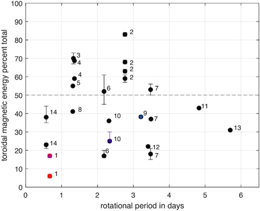
Per cent of toroidal magnetic field energy for 14 young (≲150 Myr age) solar-type stars versus rotational period. Stars with multiple epochs of ZDI observations are plotted as individual points. Error margins are shown where published. 1 – HIP 71933, F8V, age ∼15 Myr (this paper); 2 – EK Draconis, G1.5V, age ∼100 Myr (Waite et al. 2017); 3 – HD 106506, G1V, age ∼10 Myr (Waite et al. 2011); 4 – V1358 Ori, F9V, age ∼30 Myr (Willamo et al. 2022); 5 – HD 171488, G2V, age ∼30–50 Myr (Marsden et al. 2006a); 6 – HD 141943, G2, age ∼17 Myr (Marsden et al. 2011a); 7 – HD 35296, F8V, age ∼20–50 Myr (Waite et al. 2015; Willamo et al. 2022); 8 – AH Lep, G3V, age ∼20–150 Myr (Hackman et al. 2016); 9 – BD 16351, K1V, age ∼42 Myr (Folsom et al. 2016; Launhardt et al. 2022); 10 – HD 29615, G3V, age ∼30 Myr (Waite et al. 2015; Hackman et al. 2016; Willamo et al. 2022); 11 – HIP 12545, K6V, age ∼24 Myr (Folsom et al. 2016); 12 – TYC 6349-0200-1, K7, age ∼24 Myr (Folsom et al. 2016); 13 – TYC 6878-0195-1, K4V, age ∼24 Myr (Folsom et al. 2016); and 14 – HIP 89829, G5V, age ∼20 Myr (Paper I).
Magnetic fields on MS stars are believed to be driven by internal dynamos in the convection zone, and exhibit a changing and cyclic nature. Fossil magnetic fields are left over from the star’s creation and believed to be ‘frozen’ and unchanging. F-type stars cover a range of masses where the transition from fossil to dynamo magnetic field is believed to occur (Seach et al. 2022). Two F-type stars are believed to have solar-like magnetic cycles: τ Boo (Mengel et al. 2016; Jeffers et al. 2018) and HD 75332 (Brown et al. 2021). Both are mature MS stars. We have placed HIP 71933 on the pre-main sequence (PMS; see Section 2 and Fig. 1). Perhaps the static nature of the magnetic field evolution that we observe on HIP 71933 means that we have observed HIP 71933 during a relatively long low active state.
6 CONCLUSIONS
This study covers 10 yr of DI and ZDI observations of HIP 71933 from seven epochs using three different telescopes and detectors. A prominent ring of spots at +60° latitude is seen in all of the brightness maps with spot clusters that are sometimes seen at opposite east/west hemispheres. The magnetic maps from two epochs are very similar. Both exhibit dominant dipole configurations with field percentages largely consistent. There is no indication of solar-like spot migration across latitudes and while there appears to be movement of spot clusters over all seven epochs they are mostly confined to the +60° latitude ring with little latitudinal evolution of spots.
HIP 71933 shows a dominant poloidal field with multiple azimuthal wreaths. Although we have magnetic maps for only two epochs that are 2 yr apart, the azimuthal ring seems to be consistent with the spot features seen in the brightness maps. Similar wreaths are seen on other young solar analogues, but a dominant poloidal field is still uncommon on such a young rapidly rotating star.
Our magnetic field maps show a strong axisymmetric poloidal field strength and an azimuthal field wreath at the same location as a ring of spots at the +60° latitude. The field strength is strongly dipolar. There is no evidence of a solar-like magnetic cycle during our 10 yr observation period, which might indicate we have observed HIP 71933 during a period of stable activity.
ACKNOWLEDGEMENTS
The observations collected were from the following proposal IDs:
Epoch 2009.26: AAO 9A/005
Epoch 2009.34: RSAA 2090097
Epoch 2010.33: RSAA 1100078
Epoch 2011.37: ESO 087.D-0771(A)
Epoch 2012.26: RSAA 1120043
Epoch 2018.07: RSAA 4170063
Epoch 2019.46: RSAA 2190149
This work has made use of data from the European Space Agency (ESA) mission Gaia (https://www.cosmos.esa.int/gaia), processed by the Gaia Data Processing and Analysis Consortium (DPAC, https://www.cosmos.esa.int/web/gaia/dpac/consortium). Funding for the DPAC has been provided by national institutions, in particular the institutions participating in the Gaia Multilateral Agreement.
In addition, this work has made use of the NASA Astrophysics Data System (ADS) and the SIMBAD data base operated at CDS, Strasbourg, France.
DATA AVAILABILITY
The data underlying this paper will be shared on reasonable request to the corresponding author.
References
APPENDIX A: MAXIMUM ENTROPY FITS
Figs A1–A5 are the Stokes I maximum entropy fits for each epoch. The red lines are the original LSD profiles and the black lines are the fits calculated by the DI code.
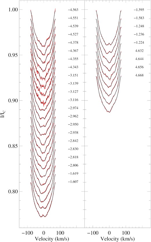
Maximum entropy fits to the Stokes I LSD profiles for AAT 2009 April Epoch 2009.26. The red lines represent the observed LSD profiles, while the black lines represent the fits to the profiles produced by the DI code. Rotational phases for each observation are indicated to the right. Each profile is shifted for graphical purposes. Observation logs report intermittent cloud cover during the first eight profiles that accounts for the noisy fits.
Maximum entropy fits to the Stokes I LSD profiles for Epoch 2009.34. The associated brightness maps are shown below the corresponding fits. The upper left-hand image is the fits using a vsini value of 76 km s−1 and shows small additional structure (dips) in the centre of most of the profiles. The upper right-hand image is the fits for a vsini of 74 km s−1, which provides a better fit. This fit results in a brightness map with additional spottedness above the +60° latitude, however there is still a lack of spots at the pole. See Section 5.5 for additional discussion.
Fig. A6 is the Stokes V maximum entropy fits for the two epochs where we obtained Stokes V data from the spectropolarimeters at the AAT SEMPOL and the LaSilla HARPSpol. Again, the red lines are the observed LSD profiles and the black lines are the fits calculated from the ZDI code.
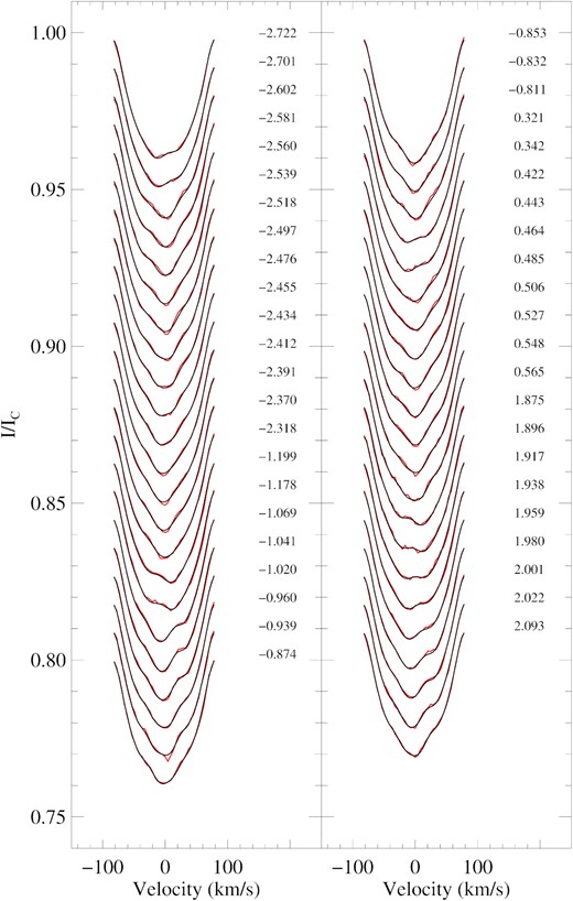
Same as Fig. A1, but for Epoch 2010.33.
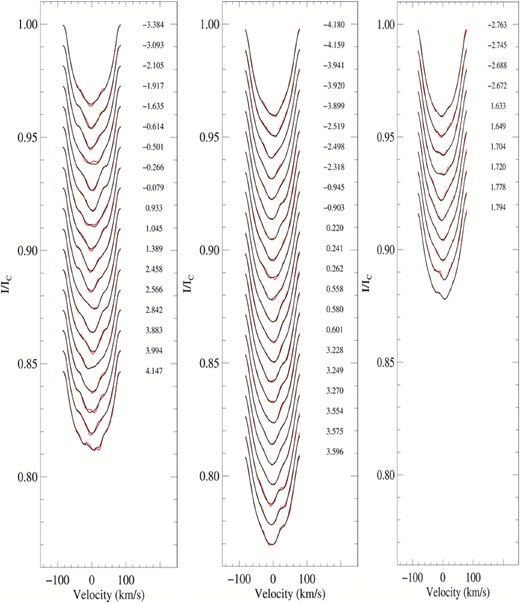
Same as Fig. A1, but for Epoch 2011.37 (left), Epoch 2012.26 (middle), and Epoch 2018.07 (right).
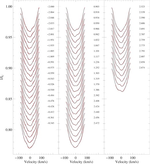
Same as Fig. A1, but for Epoch 2019.46.
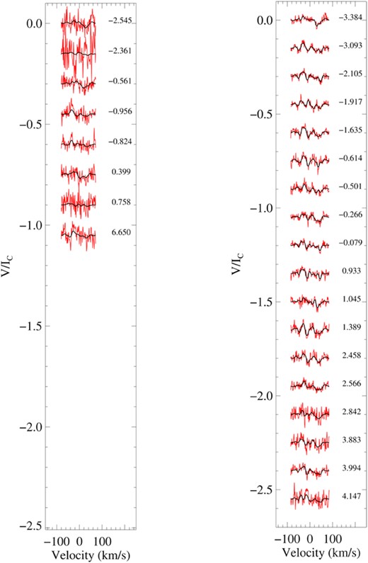
Maximum entropy fits for the Stokes V LSD profiles AAT 2009 April Epoch 2009.26 (left) and HARPSpol 2011 May Epoch 2011.37 (right). The red line represents the observed LSD profiles, while the bolder black lines represent the fits to the profiles. Each profile is shifted down for graphical purposes. The rotational phase for each observation is to the right of the profiles.
Author notes
Private astronomer.
