


ABSTRACT
GW190521 is the most massive merging binary black hole (BBH) system detected so far. At least one of the component BHs was measured to lie within the pair-instability supernova (PISN) mass gap (∼50–135 M⊙), making its formation a mystery. However, the transient observed signal allows alternative posterior distributions. There was suggestion that GW190521 could be an intermediate-mass ratio inspiral, with the component masses m1 ∼ 170 M⊙ and m2 ∼ 16 M⊙, happening to straddle the PISN mass gap. Under this framework, we perform binary population synthesis to explore the formation of GW190521-like systems via isolated binary evolution. We numerically calculate the binding energy parameter for massive stars at different metallicities, and employ them in our calculation for common envelope evolution. Our results prefer that the progenitor binaries formed in metal-poor environment with |$\rm Z\le 0.0016$|. The predicted merger rate density within redshift z = 1.1 is |${\sim} 4\times 10^{-5}{\text {--}}5\times 10^{-2} \, \rm Gpc^{-3}yr^{-1}$|. We expect that such events are potentially observable by upcoming both space and ground-based gravitational wave detectors.
1 INTRODUCTION
Detection of gravitational waves (GWs) serves us an alternative way to observe the Universe. Since the first GW event GW150914 was discovered by the ground-based detectors advanced LIGO (aLIGO) and later joined advanced Virgo, the number of binary black hole (BBH) merger events has increased to ∼100 (Abbott et al. 2016a, b, 2019, 2021; The LIGO Scientific Collaboration 2021). The observed GW signals are classified as coalescing BBH, binary neutron star, and neutron star-BH systems. GW170817 is the only GW source with electromagnetic counterpart definitely observed (Abbott et al. 2017a).
GW190521, observed on 2019 May 21 at 03:02:29 utc, is the most massive merging BBH system detected so far (Abbott et al. 2020a, b). The association of GW190521 with the candidate counterpart ZTF19abanrhr reported by Zwicky transient facility (ZTF; Graham et al. 2020) is still inconclusive (Ashton et al. 2021; Nitz & Capano 2021; Palmese et al. 2021). Under the assumption that GW190521 is a quasi-circular BBH coalescence, the estimated individual component masses are |$m_1=85_{{-14}}^{+21}{\rm M}_{\odot }$|, |$m_2=66_{{-18}}^{+17}{\rm M}_{\odot }$|, and the total mass |$150_{{-17}}^{+29}$| M⊙ within 90 per cent credible region, providing direct evidence of intermediate mass BHs (IMBHs; Abbott et al. 2020a, b). Gamba et al. (2023) drew similar results but under hyperbolic orbit hypothesis. Romero-Shaw et al. (2020) claimed that GW190521 may be an eccentric binary merger with aligned spins. Gayathri et al. (2022) interpreted this signal under the combination of both eccentricity and spin precession configuration. Barrera & Bartos (2022) estimated the ancestral mass of GW190521 and also favoured the heaviest parental BH mass in the pair-instability supernova (PISN) mass gap (between ∼50 and 135 M⊙; Yusof et al. 2013; Belczynski et al. 2016a).
Since the BH masses in GW190521-like events challenge the standard stellar evolutionary theory, there have been various models proposed to interpret their formation, including dynamical binary formation in dense stellar clusters (Rodriguez et al. 2019; Fragione, Loeb & Rasio 2020; Romero-Shaw et al. 2020; Arca-Sedda et al. 2021; Anagnostou, Trenti & Melatos 2022; Rizzuto et al. 2022; Gamba et al. 2023), additional gas accretion, and hierarchical mergers in active galactic nuclei (Tagawa, Haiman & Kocsis 2020; Tagawa et al. 2021; and references therein), and the primordial BH scenarios (De Luca et al. 2021). Alternatively, Palmese & Conselice (2021) suggested that GW190521 may be the merger of central BHs from two ultradwarf galaxies. However, the origin of this event as an isolated binary still cannot be excluded (Belczynski et al. 2020a; Farrell et al. 2021; Kinugawa, Nakamura & Nakano 2021; Tanikawa et al. 2021a). In addition, the exact boundaries of the PISN mass gap are in dispute, due to the uncertainties in stellar evolution and SN simulation, which may entail a reassessment (Woosley 2017; Farmer et al. 2019; Marchant et al. 2019; Mapelli et al. 2020; Vink et al. 2021)
Nevertheless, GW190521 is qualitatively different from previous GW sources, not only because it was the most massive GW source observed to date, but also this transient signal was found with only a short duration of approximately 0.1 s, and only around four cycles in the frequency band 30–80 Hz, so multimodal posterior distributions would be consequently ineluctable (Fishbach & Holz 2020; Bustillo et al. 2021; Nitz & Capano 2021; Estellés et al. 2022). Among them, Nitz & Capano (2021) suggested that GW190521 may be an intermediate-mass-ratio inspiral (IMRI), with the component masses of |$m_1\sim 170\, {\rm M}_{\odot }$| and |$m_2\sim 16\, {\rm M}_{\odot }$|, straddling the PISN mass gap. Comparison of the parameters derived by Abbott et al. (2020a) and Nitz & Capano (2021) are shown in Table 1.
The derived primary BH mass m1, secondary BH mass m2, total mass Mtot, dimensionless spin parameters of individual BH and effective spin parameter |$\overrightarrow{\chi _1}$|, |$\overrightarrow{\chi _2}$|, and |$\chi _{\rm eff}$| for GW190521 in the source frame. Data are cited from (Abbott et al. 2020a, A20) and (Nitz & Capano 2021, NC21), respectively. In the latter work, |$Prior_{q^{*}-M}$| denotes the prior uniform in mass ratio and total mass, |$Prior_{m_{1,2}}$| the prior uniform in component mass (m1,2), respectively. Each value is within the 90 per cent credible interval. Note here q* is the ratio of the larger mass to the smaller mass.
| Model | m1 (M⊙) | m2 (M⊙) | Mtot (M⊙) | |$|\overrightarrow{\chi _1}|$| | |$|\overrightarrow{\chi _2}|$| | χeff | |
|---|---|---|---|---|---|---|---|
| A20 | |$85_{{-14}}^{+21}$| | |$66_{{-18}}^{+17}$| | |$150_{{-17}}^{+29}$| | |$0.69_{-0.62}^{+0.27}$| | |$0.73_{-0.64}^{+0.24}$| | |$0.08_{-0.36}^{+0.27}$| | |
| Priorq − M | |$168_{-61}^{+15}$| | |$16_{-3}^{+33}$| | |$184_{-30}^{+15}$| | |$0.85_{-0.25}^{+0.11}$| | – | |$-0.51_{-0.11}^{+0.24}$| | |
| NC21 | |$Prior_{m_{1,2}}$| (q* < 4) | |$100_{-18}^{+17}$| | |$57_{-16}^{+17}$| | |$156_{-15}^{+21}$| | |$0.72_{-0.59}^{+0.25}$| | – | |$-0.16_{-0.40}^{+0.42}$| |
| |$Prior_{m_{1,2}}$| (q* > 4) | |$166_{-35}^{+16}$| | |$16_{-3}^{+14}$| | |$183_{-27}^{+15}$| | |$0.87_{-0.16}^{+0.10}$| | – | |$-0.53_{-0.12}^{+0.14}$| | |
Inspired by the results of Nitz & Capano (2021), here we attempt to interpret the formation of GW190521 assuming that it was an IMRI through isolated binary evolution, and investigate the properties of their progenitor binaries as well as the possible distributions of natal kicks on the two component BHs, which had promoted their coalescence within the Hubble time τH. The information on the BH kicks is crucial in understanding the formation of massive BHs.
The paper is structured as follows. In Section 2, we describe the main features of our binary population synthesis (BPS) models. The calculated results of BPS are presented in Section 3. We then discuss our results in Section 4, and summarize our main conclusions in Section 5.
2 MODEL
All calculations are carried out by using the BPS code bse, originally developed by Hurley, Pols & Tout (2000, 2002) and its updated version bseemp1 (Tanikawa et al. 2020, 2021b), with the extension to very massive (up to |$M\sim 1300\, {\rm M}_{\odot }$|) and extremely metal-poor stars (down to Z = 10−8 Z⊙), based on the stellar models computed by the hoshi code. The bseemp code also takes advantage of new stellar-wind and remnant-formation prescriptions, as well as the implementation of pair-instability and pulsational-pair-instability supernova (PISN/PPISN), which all play a role in stellar/binary evolution.
2.1 Stellar wind mass-loss
The masses of BHs are predominantly set by their pre-SN masses, which are mainly affected by stellar wind mass-loss and binary interactions. Mass-loss via stellar winds can significantly influence the fate of massive stars (Fryer et al. 2002). Here, we use the semi-empirical stellar wind prescription (referred as Vink et al. winds) in Belczynski et al. (2010), and consider metallicity dependence for luminous blue variables (LBVs; Tanikawa et al. 2021b). It has been demonstrated that this wind prescription results in more massive pre-SN objects and heavier BHs compared with the traditional one (Belczynski et al. 2010). We ignore the influence of stellar rotation on wind loss.
For massive O and B stars, the wind mass-loss rate |$\dot{M}_{\rm W}$| in units of |${\rm M}_{\odot }\, {\rm yr}^{-1}$| is (Vink, de Koter & Lamers 2001)
with |$12\,500\, {\rm K} \le T \le 25\,000$| K. Here, L and M are the luminosity and the mass in solar units, respectively, Z is metallicity, T is the effective temperature of the star, and V = v∞/vesc = 1.3 is the ratio of the wind velocity at infinity to the escape velocity from the star.
For hotter stars with |$25\,000\, {\rm K} \le T \le 50\,000$| K,
with V = 2.6.
For LBVs beyond the HD limit (Humphreys R. M., Davidson K.1994) (L > 6 × 10⁵ and 10−5RL0.5 > 1.0, where R is the stellar radius in solar units),
where fLBV = 1.5 is a calibration factor. Obviously, lower flbv results in weaker LBV wind, leaving a heavier remnant (Belczynski et al. 2010).
The reduced Wolf–Rayet star mass-loss with small H-envelope mass takes the form of metallicity-dependent power law,
with
m = 0.86 describing the dependence of wind mass-loss on metallicity, and MHe the He core mass of the star (Vink & de Koter 2005).
For other stars, we use the wind prescriptions described in Hurley et al. (2000).
2.2 Black hole formation
Stars are powered by burning their core fuels to heavier elements step by step. For massive stars, this process continues until an iron core is built up in the stellar centre. As the fusion of iron does not produce further energy, burning halts. Later, stars contract on their own weights, leading to accelerating processes of electron capture and core element dissociation. These processes dramatically reduce the pressure that should have resisted their self-gravity, triggering a runaway core-collapse process. Collapse halted by nuclear forces and neutron degeneracy pressure and form a proto-NS. Explosion launches after the ‘bounce’ of the core, and part or all of the expelled stellar envelope will fall back and accrete on to the proto-NS, which may eventually collapse into a BH (Fryer et al. 2012).
There are still many uncertainties associated with the physics of the SN mechanism. Here, we use the delayed SN prescription of Fryer et al. (2012; hereafter F12-delayed), where the explosion did not launch until over ∼250 ms after the collapse. For a massive star with pre-SN mass of MSN and CO core mass of MCO, the expected BH remnant mass MBH is estimated as follows:
where MBH,bar is the baryonic mass,2Mproto is the proto-NS mass after core collapse,
and Mfb is the amount of material falls back to the proto-NS,
where |$f_1=0.133 - {0.093 \over M-M_{\rm proto}}$|, and f2 = −11f1 + 1. We define ffb = Mfb/(MSN − Mproto) as the fallback fraction during the BH formation, which is important in determining the BH’s natal kick in some kick prescriptions.
Stars with He core mass MHe in the range of |${\sim} 35{\!-\!}60\, {\rm M}_{\odot }$| are subjected to PPISNe (Heger & Woosley 2002; Yusof et al. 2013; Belczynski et al. 2016a; Leung, Nomoto & Blinnikov 2019; Marchant et al. 2019; Stevenson et al. 2019), with most of the mass above the core stripped by a set of pulsations, leaving behind the BHs with mass significantly smaller than they would be if only accounting for the core-collapse SNe. We adopt the prescription of PPISNe in Marchant et al. (2019), who computed an array of H-free metal-poor (0.1 Z⊙) single-star models based on the standard 12C(α, γ)O16 reaction rate to evaluate the PPISN mass-loss, and the BH masses after PPISNe can be estimated as:
where ζi are the polynomial fitting coefficients of Marchant et al. (2019)’s PPISN prescription given by Stevenson et al. (2019; as listed in Table 2). Note that the remnant mass is a non-monotonic function of the initial stellar mass.
Coefficients in Equation 8.
| Coefficient | Value |
|---|---|
| ζ0 | 7.39643451 × 10³ |
| ζ1 | −1.13694590 × 10³ |
| ζ2 | 7.45060098 × 101 |
| ζ3 | −2.69801221 × 100 |
| ζ4 | 5.83107626 × 10⁻² |
| ζ5 | −7.52206933 × 10⁻⁴ |
| ζ6 | 5.36316755 × 10⁻⁶ |
| ζ7 | −1.63057326 × 10⁻⁸ |
| Coefficient | Value |
|---|---|
| ζ0 | 7.39643451 × 10³ |
| ζ1 | −1.13694590 × 10³ |
| ζ2 | 7.45060098 × 101 |
| ζ3 | −2.69801221 × 100 |
| ζ4 | 5.83107626 × 10⁻² |
| ζ5 | −7.52206933 × 10⁻⁴ |
| ζ6 | 5.36316755 × 10⁻⁶ |
| ζ7 | −1.63057326 × 10⁻⁸ |
More massive stars with |$60\, {\rm M}_{\odot }\le M_{\rm He} \le 135\, {\rm M}_{\odot }$| are subjected to PISNe, the entire star is completely disrupted with no remnant left.3 Stars with |$M_{\rm He}\gt 135\, {\rm M}_{\odot }$| are assumed to directly collapse to BHs.
2.3 Supernova kicks
As BH natal kicks suffer from a lack of stringent constraints from both observation and theory (Willems et al. 2005; Fragos et al. 2009; Repetto, Davies & Sigurdsson 2012; Repetto & Nelemans 2015; Belczynski et al. 2016c; Mandel 2016; Repetto, Igoshev & Nelemans 2017), we adopt three different natal kick prescriptions (kickF) as follows (Banerjee et al. 2020):
Standard fallback-controlled kick (hereafter k1)
Convection-asymmetry-driven natal kick (hereafter k2)
The BH natal kicks are produced by the convection asymmetries of the collapsing SN core (Scheck et al. 2004; Fryer & Kusenko 2006), soIn this equation, kconv is an efficiency factor (somewhere between 2 and 10, and we set kconv = 5 here), and <MNS > is a typical NS mass, taken to be |$1.4\, {\rm M}_{\odot }$|.(10)$$\begin{eqnarray} v_{\rm kick,BH} = \left\lbrace \begin{array}{ll}v_{\rm kick,NS}\frac{\lt M_{\rm NS}\gt }{M_{\rm BH}}(1-f_{\rm fb}) & {\rm if}\ M_{\rm CO} \le 3.5\, {\rm M}_{\odot },\\ k_{\rm conv}v_{\rm kick,NS}\frac{\lt M_{\rm NS}\gt }{M_{\rm BH}}(1-f_{\rm fb}) & {\rm if}\ M_{\rm CO}\ \gt 3.5\, {\rm M}_{\odot }.\\ \end{array} \right. \end{eqnarray}$$Neutrino-driven natal kick (hereafter k3)
where Meff (usually between |$5$| and |$10\, {\rm M}_{\odot }$|) is the effective remnant mass, and we let |$M_{\rm eff} = 7\, {\rm M}_{\odot }$| (Banerjee et al. 2020).
To constrain the allowed velocity range in different kick prescriptions, we take a flat distribution of vkick,NS in the range of |$0{\!-\!}1000\rm \, kms^{-1}$|, and assume that the SN kicks are isotropically distributed and the mass is instantaneously lost at the moment of SN. Then vkick,BH can be obtained from the equations mentioned above for different kick prescriptions. When we calculate the merger rate density we adopt a more realistic, predetermined Maxwellian distribution for the NS kick velocity.
Note also that in both k1 and k2 prescriptions, there is no natal kick for BHs formed through direct core collapse (ffb = 1.0).
2.4 Natal BH spins
The BH spins are modelled following Tanikawa et al. (2021b). We assume zero natal spin of the zero-age main sequence (ZAMS) star, which then evolves due to stellar evolution, stellar winds, and binary interactions. Newborn BHs inherit their progenitor’s spin angular momenta, except for the PPISN events where zero BH spin parameters are assumed. If the spin angular momenta of the BH progenitors are larger than those of extreme Kerr BHs, the BH spin parameters are forced to be unity. Thus, the BH spin parameter can be expressed as:
where |$\overrightarrow{S}$| and M are the spin angular momentum and the mass of the BH progenitor just before its collapse, respectively, c the speed of light, G the gravitational constant, and |$\overrightarrow{L}$| the binary orbital angular momentum.
The BH natal kicks would tilt |$\overrightarrow{\chi }$| from |$\overrightarrow{L}$|. We choose the coordinate in which the z-axis is parallel to the orbital angular momentum vector just before the second BH formed, that is, the normalized orbital angular momentum vector is (0, 0, 1). Then, the normalized spin vectors of the first and second formed BH |$\overrightarrow{\chi _1}$| and |$\overrightarrow{\chi _2}$| can be written as:
where |$\theta _1^{\prime }$| is the angle between the first BH spin vector and binary orbital angular momentum vector just before the second BH forms, |$\phi _1^{\prime }$| is randomly chosen between 0 and 2π. Finally, the angles θ1 (θ2) between the first (second) formed BH spin and the final BBH orbital angular momentum vector just after the second BH formation can be expressed as:
and we do not consider possible BH spin alignment with orbital angular momentum due to tides or mass transfer. The effective spin parameter χeff of merging BBHs which reflects the spin-orbit alignment is defined as:
where m1 and m2 are the merging BBH masses.
2.5 Common-envelope evolution
For semidetached binaries, a common-envelope (CE) phase occurs when the mass transfer becomes dynamically unstable or when the two stars (with at least one of them being a giant-like star) collide at orbital periastron before Roche lobe overflow (RLOF; Hurley et al. 2002). The CE phase plays a fundamental role in the formation of GW190521-like systems. Due to the extreme initial mass ratio q ∼ 0.1, mass transfer from the massive primary star to the secondary star is usually dynamically unstable and leads to CE evolution. In addition, systems with large orbital eccentricities are likely to collide at periastron. Binaries can survive the CE phase if the accretor’s orbital energy is large enough to unbind the stellar envelope.4 Here, we adopt the αCEλ formalism (de Kool 1990), which can be expressed as:
where the envelop’s binding energy,
Here, αCE is the efficiency of converting the released orbital energy to eject CE, λ the binding energy parameter depending on envelope’s structure (see Ivanova et al. 2013, for details), M1, Mc, and Menv = (M1 − Mc) the masses of the donor, donor’s core, and envelope, respectively, M2 the mass of the accretor, ai,CE and af,CE the binary separation before and after the CE phase, respectively, RRL the donor’s RL radius at the onset of the CE phase, U the specific internal energy (including both thermal and recombination energies) of envelope, and αth the efficiency with which thermal energy can be used to eject the envelope. In this work, αth = 1 is assumed.
Following Xu & Li (2010) and Wang, Jia & Li (2016), we calculate the binding energy parameter λ for stars more massive than |$60\, {\rm M}_{\odot }$| with metallicity Z = 0.02, 0.001, and 0.0001 using the stellar evolution code mesa (version 11701; Paxton et al. 2011, 2015, 2018, 2019). We then calculate λb and λg with Ebind including and excluding the internal energy term U, respectively. Detailed models and fitting results of λ are presented in Appendix A. We only use λb in our following population synthesis calculations.
In order to explore the dependence of our results on αCE, we have run a set of simulations with αCE = 0.5, 1.0, and 3.0 (αCE > 1.0 would occur when additional energy or angular momentum depositing into the giant’s envelope is considered, see e.g. Soker 2004).
2.6 Population synthesis
We perform BPS simulations of binary stars with the bseemp code. We assume that all the stars are in binaries, and exclude binary systems with at least one of the two components fills its RL at the beginning of evolution. The initial masses Mi,1 of the primary stars are distributed in the range of |$[300:900]\, {\rm M}_{\odot }$| following the Kroupa (2001) law. For the masses of the secondary stars Mi,2 = qMi,1, we adopt a flat distribution of the mass ratio q (Sana et al. 2012), and limit |$M_{\rm i,2}= [10:60]\, {\rm M}_{\odot }$|. We consider various metallicities with Z = 0.0002, 0.0004, 0.0008, 0.0016, 0.0032, 0.0063, 0.0126, and 0.02. The initial orbital semimajor axis ai is assumed to be distributed uniformly in logspace and restricted to |$[3:10^{7}]\, {\rm R}_{\odot }$|. We consider both initially circular (hereafter ‘ei = 0’ model) and eccentric (hereafter ‘ei = 0 ∼ 1’ model) orbit configurations in each case. In the latter model, the eccentricity follows a uniform distribution between 0 and 1.
We focus only on GW190521-like systems with the primary and secondary BH masses |$m_1 = [150:180]\, {\rm M}_{\odot }$| and |$m_2 = [10:20]\, {\rm M}_{\odot }$|, so it is reasonable to only simulate binaries with a limited initial parameter ranges, and make sure that the simulated population parameters are complete to form GW190521-like systems.
Incorporating the three kick prescriptions (kickF = k1, k2, and k3) and three values of αCE = (0.5, 1.0, and 3.0), we perform 18 sets of BPS simulations of 107 primordial binaries at each metallicity. We list the initial parameters of models with Z ≤ 0.0016 in Table 3. For higher metallicity, we found that there is no GW190521-like system formed in our simulation.
The initial parameters of our BPS models for both ‘ei = 0’ and ‘ei = 0 ∼ 1’ models. Here, Mi,1 and Mi,2 are the initial primary and secondary masses, respectively, and ai is the initial orbital semimajor axis, all in solar units. Because there is no BH as massive as |${\sim} 150\, {\rm M}_{\odot }$| formed in our calculation at Z ≥ 0.0032, owing to the significant wind mass-loss and PISN under our evolutionary assumptions, we only display the runs of Z = 0.0002, 0.0004, 0.0008, and 0.0016 which can form BHs with mass in the range of interest.
| Z | 0.0002 | 0.0004 | 0.0008 | 0.0016 |
|---|---|---|---|---|
| |$M_{\rm i,1}\, [{\rm M}_{\odot }]$| | 300–450 | 350–500 | 400–700 | 500–900 |
| |$M_{\rm i,2}\, [{\rm M}_{\odot }]$| | 20–60 | |||
| |$a_{\rm i}\, [{\rm R}_{\odot }]$| | 103.5–107 | |||
| kickF | k1, k2, k3 | |||
| αCE | 0.5, 1.0, 3.0 | |||
We assume a non-conservative mass transfer prescription with the accretion efficiency being 0.5. We follow the evolution of the primordial binaries until the formation of BBHs. For a newborn BBH system with component masses m1 and m2, orbital semimajor axis a0 and eccentricity e0, the inspiral time delay tinspiral (a0, e0), namely the time elapsed between the birth and the merger of the BBH, can be calculated (Peters 1964):
where
and
2.7 Merger rate density
We then follow the procedure of Giacobbo & Mapelli (2018b) to estimate the cumulative merger rate density |$\mathcal {R}(z\le z_{\rm det})$| of GW190521-like BBH systems within a given redshift zdet,
where tlb(z) is the look-back time for binaries formed at redshift z, |$M_{*} \simeq 0.55\, {\rm M}_{\odot }$| the mean mass of a stellar system in population with the Kroupa (2001) IMF, fbin = 0.7 the fraction of stars in binaries (Sana et al. 2012), Wb the contribution of specific binaries we are interested in (Hurley et al. 2002), |$\mathcal {SFR}(z)$| the cosmic star formation rate density as a function of z, usually peaked at z ∼ 1.9 and declined exponentially at later time. We assume that in our models the star formation commenced at z = 15.
The BBH progenitor binaries formed at redshift zf would merge as GW sources at zm (zm < zf) after a delay time tdelay, which is defined as the interval between the formation of the progenitor binary and the coalescence of the BBH, i.e. tdelay = tinspiral + T, where |$T\lt 10 \,\,\rm Myr$| is the lifetime of progenitor system, if the orbital angular momentum loss is efficient enough. So, we can get the look-back times at their formation
where E(z) = [Ωm(1 + z)3 + Ωλ]1/2, and at their merger
In our calculation, we employ the flat |$\rm \Lambda CDM$| model with |$H_0=67.8\, \rm kms^{-1}Mpc^{-1}$|, Ωm = 0.3, and Ωλ = 0.7, where |$\tau _{\rm H} = 1/H_0=14.4\, \rm Gyr$| is the Hubble time (Planck Collaboration 2016). We adopt the cosmic |$\mathcal {SFR}(z)$| density in Madau & Dickinson (2014):
and the metallicity as a function of redshift z in Belczynski et al. (2016b). For the portions of distributions extending beyond the metallicity range [0.0002, 0.02], we use the recorded information of the systems at Z = 0.0001 or 0.02. We exclude the mergers in the near future (tmerg < 0).
2.8 Character strain
The characteristic strain of the GW signals at the nth harmonic can be calculated following Kremer et al. (2019),
where |$M_{c,z} = M_c(1+z) = \frac{(m_1m_2)^{3/5}}{(m_1+m_2)^{1/5}}(1+z)$| is the observed chirp mass at redshift z, and DL is the luminosity distance to the source calculated by
|$f_{n,z}=\frac{f_n}{1+z}=\frac{nf_{\rm orb}}{1+z}$| is the observed frequency of the nth harmonic (fn is the frequency of the nth harmonic in the source frame and forb is the source-fame orbital frequency), g(n, e) is the function of eccentricity, and F(e) is the eccentricity correction factor defined to be (Peters & Mathews 1963):
As the GW power is sharply peaked at the peak frequency fpeak (Peters & Mathews 1963), we calculate the characteristic strain of our modelled GW sources at the peak frequency fpeak for simplicity (Hamers 2021),
Thus, n = npeak = fpeak/forb (Wang, Tanikawa & Fujii 2022).
During the inspiral, the eccentricity changes due to gravitational radiation (Peters 1964),
and the orbital separation evolves with eccentricity
where c0 is determined by the initial condition a(e0) = a0 (see equation 19).
3 RESULTS
For each model, we regard the merging BBHs with component masses |$m_1=[150:180]\, {\rm M}_{\odot }$| and |$m_2=[10:20]\, {\rm M}_{\odot }$| as GW190521-like systems (as shown in Fig. 1). According to the analysis of Nitz & Capano (2021), the primary BH mass in GW190521 is |${\sim} 170\, {\rm M}_{\odot }$|. We simulate binary evolution with the primary mass |${\le} 900\, {\rm M}_{\odot }$| at different metallicities and find that such massive BHs can only form at relatively low metallicities (Z ≤ 0.0016), with the pre-collapse core-helium masses heavier than |$135\, {\rm M}_{\odot }$|, while stars at higher metallicity (Z ≥ 0.0032) will undergo PISNe, triggering complete disruption of the star and leaving no compact remnants. This is because stars formed in lower metallicity environments can reach higher central temperatures, which results in larger core masses than their counterparts at higher metallicity. So, our following discussions only refer to the data set of the models with Z ≤ 0.0016.
The posterior distribution of GW190521 from Nitz & Capano (2021) under Priorq − M prior, overlaid yellow region is the component masses of our calculated GW190521-like systems.
Table 4 lists the predicted numbers of GW190521-like systems and kick velocity distributions under different conditions. Their main features can be summarized as follows:
Most of GW190521-like systems form through the ‘MT + CE’ channel. Here, ‘MT’ means that stars in a binary interact via stable RLOF or wind accretion, and the ‘CE’ phase is triggered by eccentric collision of both stars at periastron instead of dynamically unstable mass transfer caused by the expansion of the donor star. Binary stars in eccentric orbits may collide at periastron before either one fills its RL, and such collisions lead to CE evolution if at least one of the stars is a giant-like star (Hurley et al. 2002). Thus, only the k3 kick prescription that produces non-zero BH1 natal kick velocities works in this channel. Besides, the number of BBH mergers decreases as αCE increases, because larger αCE leads to wider orbits after the CE phase, making it more difficult for the BBHs to merge. To reproduce GW190521-like systems in this channel requires |$v_{\rm kick,1} \simeq 0{\!-\!}50 \, \rm kms^{-1}$| and |$v_{\rm kick,2} \simeq 0{\!-\!}700 \, \rm kms^{-1}$|.
Only about 0.1 per cent of GW190521-like systems form through ‘MT + MT’ channel. The systems with moderate low eccentricities can avoid collision at periastron until the BBH formation. So, this channel is independent of the value of αCE. The predicted natal kick velocities are vkick,1 = 0 and |$v_{\rm kick,2} \simeq 30{\!-\!}90 \, \rm kms^{-1}$| (kickF = k1, k2), and |$v_{\rm kick,1} \simeq 0{\!-\!}50 \, \rm kms^{-1}$| and |$v_{\rm kick,2} \simeq 16{\!-\!}400 \, \rm kms^{-1}$| (kickF = k3).
For very low mass ratio binaries (q < 0.1), the secondary star usually does not have enough energy to drive off the CE if it is triggered by dynamically unstable MT, so there is no system formed via the ‘CE + MT’ channel in the ‘ei = 0’ model. In the ‘ei = 0 ∼ 1’ model, the non-zero eccentricity makes CE evolution possible just like in the ‘MT + CE’ channel. The number of surviving systems also decreases with increasing αCE. The predicted natal kick velocities are vkick,1 = 0 and |$v_{\rm kick,2}\simeq 100{\!-\!}400 \, \rm kms^{-1}$| (kickF = k1, k2), and |$v_{\rm kick,1}\simeq 0{\!-\!}45 \, \rm kms^{-1}$| and |$v_{\rm kick,2} \simeq 60{\!-\!}420 \, \rm kms^{-1}$| (kickF = k3).
No GW190521-like system form though the ‘CE + CE’ channel.
Numbers of GW190521-like systems evolved via each evolution channel from ZAMS binaries to BBHs. ‘MT + CE’: system experiences stable mass transfer (via RLOF or wind mass-loss) and later once CE phase, ‘MT + MT’: system without CE evolution, ‘CE + MT’: system experiences once CE phase and later stable RLOF or wind accretion, ‘CE + CE’: system experiences twice CE phases. The corresponding minimum and maximum of vkick,1 and vkick,2 are also shown following their numbers.
| αCE | kickF | MT + CE | MT + MT | CE + MT | CE + CE |
|---|---|---|---|---|---|
| vkick (|$\rm kms^{-1}$|) | |||||
| k1 | – | 19 | – | – | |
| vkick,1, vkick,2 | 0, 41.305 − 63.905 | ||||
| 0.5 | k2 | – | 32 | – | – |
| vkick,1, vkick,2 | 0, 36.9 − 80.6 | ||||
| k3 | 17279 | 26 | – | – | |
| vkick,1, vkick,2 | 1.695 − 46.487, 0.004 − 691.626 | 0.015 − 40.476, 16.843 − 114.77 | |||
| k1 | – | 19 | – | – | |
| vkick,1, vkick,2 | 0, 41.305 − 63.905 | ||||
| 1.0 | k2 | – | 32 | – | – |
| ei = 0 | vkick,1, vkick,2 | 0, 36.9 − 80.6 | |||
| k3 | 14862 | 28 | – | – | |
| vkick,1, vkick,2 | 2.499 − 46.499, 0.028 − 691.626 | 3.942 − 40.476, 21.428 − 383.477 | |||
| k1 | – | 20 | – | – | |
| vkick,1, vkick,2 | 0, 41.305 − 63.905 | ||||
| 3.0 | k2 | – | 32 | – | – |
| vkick,1, vkick,2 | 0, 36.9 − 80.6 | ||||
| k3 | 8671 | 24 | – | – | |
| vkick,1, vkick,2 | 1.969 − 46.605, 0.111 − 693.735 | 2.265 − 44.953, 19.369 − 214.626 | |||
| k1 | – | 11 | 134 | – | |
| vkick,1, vkick,2 | 0, 36.286 − 72.81 | 0, 171.063 − 394.826 | |||
| 0.5 | k2 | – | 22 | 105 | – |
| vkick,1, vkick,2 | 0, 30.589 − 90.388 | 0, 166.311 − 413.726 | |||
| k3 | 18394 | 17 | 235 | – | |
| vkick,1, vkick,2 | 0.379 − 46.509, 0.092 − 697.315 | 4.734 − 45.848, 34.513 − 142.709 | 0.092 − 44.373, 99.196 − 422.095 | – | |
| k1 | – | 10 | 45 | – | |
| vkick,1, vkick,2 | 0, 36.286 − 72.81 | 0, 146.125 − 249.277 | |||
| 1.0 | k2 | – | 24 | 63 | – |
| ei = 0 ∼ 1 | vkick,1, vkick,2 | 0, 30.589 − 90.388 | 0, 134.284 − 301.761 | ||
| k3 | 15887 | 26 | 63 | – | |
| vkick,1, vkick,2 | 0.149 − 46.187, 0.032 − 687.68 | 1.202 − 46.288, 19.738 − 152.097 | 0.021 − 41.708, 102.228 − 260.19 | ||
| k1 | – | 11 | 19 | – | |
| vkick,1, vkick,2 | 0, 36.286 − 72.81 | 0,104.945 − 171.183 | |||
| 3.0 | k2 | – | 23 | 22 | – |
| vkick,1, vkick,2 | 0, 30.589 − 90.388 | 0, 109.604 − 186.818 | |||
| k3 | 9250 | 15 | 28 | – | |
| vkick,1, vkick,2 | 0.899 − 46.42, 0.017 − 675.649 | 10.485 − 45.848, 19.738 − 190.988 | 2.076 − 41.044, 59.636 − 247.057 |
Table 5 presents the inferred parameters of GW190521-like systems that will merge within z = 1.1 and their progenitors. As most of them are formed with kickF = k3, we only show the results with the k3 prescription. The number and its subscripts and superscripts represent the 50th, 16th, and 84th percentiles of each parameter. It is seen that the results do not show significant differences in the ‘ei = 0’ and ‘ei = 0 ∼ 1’ models.
The inferred parameters of GW190521-like systems (merged within z = 1.1) and their progenitors. The values and uncertainties of each parameter indicate the 50th, 16th, and 84th percentiles of the posterior samples. Mi,1, Mi,2, ai, and ei are the initial component masses, orbital semimajor axis, and eccentricity of GW190521-like system’s progenitors, respectively. m1, m2, a0, and e0 are those of the GW190521-like systems. vkick,1 (vkick,2) the natal kick velocities of the first (second) formed BHs and tdelay the delay time of GW190521-like systems. Runs for kickF = k3.
| Model | αCE | Mi,1 (M⊙) | Mi,2 (M⊙) | log ai (R⊙) | ei | log a0 (R⊙) |
|---|---|---|---|---|---|---|
| 0.5 | |$433.71_{-55.03}^{+147.60}$| | |$42.95_{-2.42}^{+3.01}$| | |$4.16_{-0.28}^{+0.39}$| | 0 | |$1.89_{-0.08}^{+0.17}$| | |
| ei = 0 | 1.0 | |$419.53_{-46.43}^{+198.54}$| | |$42.80_{-3.14}^{+3.68}$| | |$4.19_{-0.28}^{+0.36}$| | 0 | |$1.88_{-0.07}^{+0.10}$| |
| 3.0 | |$444.77_{-67.40}^{+224.67}$| | |$37.83_{-2.79}^{+4.08}$| | |$4.16_{-0.24}^{+0.35}$| | 0 | |$1.84_{-0.07}^{+0.09}$| | |
| 0.5 | |$450.16_{-69.61}^{+232.91}$| | |$43.07_{-3.13}^{+3.11}$| | |$4.19_{-0.29}^{+0.34}$| | |$0.49_{-0.32}^{+0.24}$| | |$1.90_{-0.09}^{+0.54}$| | |
| ei = 0 ∼ 1 | 1.0 | |$422.61_{-47.97}^{+206.80}$| | |$43.18_{-3.38}^{+3.33}$| | |$4.22_{-0.28}^{+0.37}$| | |$0.47_{-0.33}^{+0.24}$| | |$1.88_{-0.07}^{+0.15}$| |
| 3.0 | |$442.68_{-67.86}^{+229.05}$| | |$37.71_{-2.57}^{+4.36}$| | |$4.22_{-0.29}^{+0.44}$| | |$0.46_{-0.28}^{+0.27}$| | |$1.84_{-0.07}^{+0.11}$| | |
| e0 | m1 (M⊙) | m2 (M⊙) | |$v_{\rm kick,1}~(\rm kms^{-1})$| | |$v_{\rm kick,2}~(\rm kms^{-1})$| | |$t_{\rm delay}~(\rm Gyr)$| | – |
| |$0.35_{-0.25}^{+0.29}$| | |$164.14_{-10.22}^{+8.36}$| | |$17.26_{-1.52}^{+1.58}$| | |$33.77_{-11.27}^{+5.90}$| | |$229.66_{-165.78}^{+109.71}$| | |$5.65_{-1.84}^{+3.24}$| | – |
| |$0.27_{-0.18}^{+0.31}$| | |$163.55_{-8.30}^{+9.28}$| | |$17.15_{-1.82}^{+2.00}$| | |$34.03_{-10.45}^{+6.13}$| | |$180.34_{-117.76}^{+165.35}$| | |$5.94_{-2.09}^{+3.09}$| | – |
| |$0.24_{-0.17}^{+0.27}$| | |$164.13_{-9.38}^{+9.84}$| | |$14.61_{-2.67}^{+1.93}$| | |$33.83_{-8.96}^{+6.22}$| | |$186.98_{-134.74}^{+163.48}$| | |$5.81_{-2.06}^{+3.14}$| | – |
| |$0.38_{-0.27}^{+0.51}$| | |$165.51_{-11.03}^{+8.21}$| | |$17.24_{-1.56}^{+1.61}$| | |$27.56_{-12.94}^{+10.36}$| | |$220.53_{-143.98}^{+119.35}$| | |$5.76_{-2.00}^{+2.94}$| | – |
| |$0.28_{-0.19}^{+0.38}$| | |$165.05_{-8.83}^{+8.21}$| | |$17.32_{-1.82}^{+1.61}$| | |$28.94_{-13.62}^{+8.70}$| | |$184.35_{-121.13}^{+160.26}$| | |$5.92_{-2.05}^{+3.08}$| | – |
| |$0.24_{-0.17}^{+0.32}$| | |$164.34_{-9.21}^{+10.80}$| | |$14.62_{-2.45}^{+2.10}$| | |$27.68_{-14.17}^{+10.00}$| | |$173.27_{-122.20}^{+201.65}$| | |$5.80_{-2.05}^{+3.13}$| | – |
The analysis of Abbott et al. (2020a, b) suggested that GW190521 merged at the redshift of |$0.82_{-0.34}^{+0.28}$|, while Nitz & Capano (2021) predicted a luminosity distance of |$1.06_{-0.28}^{+1.4}\rm Gpc$| (|$z\simeq 0.21_{-0.05}^{+0.23}$|). According to their restrictions on the redshift, we display the calculated merger rate density |$\mathcal {R}$| of GW190521-like systems at z ≤ 0.48 and z ≤ 1.1 in Table 6, which lie in the range of |$4\times 10^{-5}{\!-\!}5\times 10^{-2} \, \rm Gpc^{-3}yr^{-1}$|. As mentioned above, the merger rate density with the k3 kick prescription is much more than with the k1 or k2 prescription.
The calculated merger rate density of GW190521-like systems with the natal kick drawn from a Maxwell distribution of NS kick velocity (σNS = 265 kms−1). The 3rd–6th columns present the numbers of BBHs with the progenitor systems formed at relevant metallicity and merged in local Universe with zm ≤ 0.48 and 1.1 (in parentheses) per |$\rm Gpc^3$| per |$\rm year$|. The last column lists the cumulated merger rate densities taking into account cosmic evolution.
| αCE | kickF | Z = 0.0002 | Z = 0.0004 | Z = 0.0008 | Z = 0.0016 | |$\mathcal {R}(z_{\rm m}\le 0.48)((z_{\rm m}\le 1.1)$|) | |
|---|---|---|---|---|---|---|---|
| (|$\rm Gpc^{-3}yr^{-1}$|) | |||||||
| ei = 0 | |||||||
| k1 | - (-) | - (-) | - (-) | 4.067e-05 (4.067e-05) | 4.067e-05 (4.067e-05) | ||
| 0.5 | k2 | 9.087e-05 (2.111e-04) | 1.180e-04 (3.193e-04) | 3.089e-04 (6.838e-04) | 7.771e-05 (3.457e-04) | 5.955e-04 (1.560e-03) | |
| k3 | 2.668e-04 (1.738e-03) | 2.498e-03 (8.888e-03) | 3.847e-03 (1.583e-02) | 1.192e-03 (5.759e-03) | 7.803e-03 (3.221e-02) | ||
| k1 | - (-) | - (-) | - (-) | 6.889e-05 (6.889e-05) | 6.889e-05 (6.889e-05) | ||
| 1.0 | k2 | 9.087e-05 (2.112e-04) | 1.180e-04 (3.193e-04) | 3.089e-04 (6.838e-04) | 7.771e-05 (3.457e-04) | 5.955e-04 (1.560e-03) | |
| k3 | 1.380e-03 (5.235e-03) | 2.498e-03 (9.151e-03) | 4.352e-03 (1.516e-02) | 2.099e-03 (7.390e-03) | 1.033e-02 (3.694e-02) | ||
| k1 | - (-) | - (-) | - (-) | 5.724e-05 (5.724e-05) | 5.724e-05 (5.724e-05) | ||
| 3.0 | k2 | 9.087e-05 (2.112e-04) | 1.180e-04 (3.193e-04) | 3.089e-04 (6.838e-04) | 7.771e-05 (3.457e-04) | 5.955e-04 (1.560e-03) | |
| k3 | 1.352e-03 (4.831e-03) | 2.183e-03 (8.117e-03) | 4.267e-03 (1.602e-02) | 6.142e-03 (2.230e-02) | 1.394e-02 (5.127e-02) | ||
| ei = 0 ∼ 1 | |||||||
| k1 | - (-) | - (-) | - (-) | 2.841e-03 (8.544e-03) | 2.841e-03 (8.544e-03) | ||
| 0.5 | k2 | 1.639e-05 (9.837e-05) | 0.0 (1.582e-04) | 5.693e-05 (5.693e-05) | 1.0750e-03 (3.023e-03) | 1.148e-03 (3.337e-03) | |
| k3 | 2.431e-04 (2.727e-03) | 2.392e-03 (9.022e-03) | 4.323e-03 (1.637e-02) | 4.364e-03 (1.726e-02) | 1.132e-02 (4.537e-02) | ||
| k1 | - (-) | - (-) | - (-) | 1.208e-03 (4.552e-03) | 1.208e-03 (4.552e-03) | ||
| 1.0 | k2 | 1.639e-05 (9.837e-05) | 0.0 (1.582e-04) | 5.693e-05 (5.693e-05) | 4.771e-04 (1.449e-03) | 5.550e-04 (1.763e-03) | |
| k3 | 1.422e-03 (5.271e-03) | 2.354e-03 (8.712e-03) | 4.438e-03 (1.632e-02) | 2.927e-03 (1.445e-02) | 1.114e-02 (4.476e-02) | ||
| k1 | -(-) | -(-) | - (-) | 3.320e-04(1.071e-03) | 3.320e-04 (1.071e-03) | ||
| 3.0 | k2 | 1.639e-05 (9.837e-05) | 0.0 (1.582e-04) | 5.693e-05 (5.693e-05) | 1.048e-03 (2.369e-03) | 1.121e-03 (2.683e-03) | |
| k3 | 1.370e-03 (4.888e-03) | 2.141e-03 (7.988e-03) | 4.024e-03 (1.549e-02) | 6.149e-03 (2.249e-02) | 1.369e-02 (5.085e-02) | ||
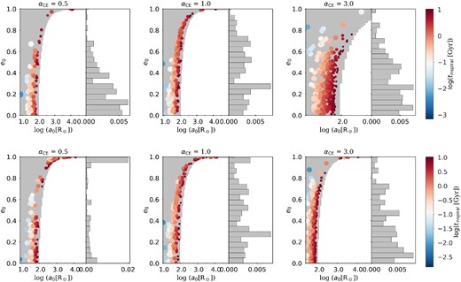
Fig. 2 shows the distribution of e0 and a0 at the birth of the BBHs (with Z = 0.0002 and kickF = k3). The upper and lower panels correspond to the ‘ei = 0’ and ‘ei = 0 ∼ 1’ models, and the left-, middle-, and right-hand panels correspond to αCE = 0.5, 1.0, and 3.0, respectively. The distribution of e0 tends to be wider with increasing αCE in both ‘ei = 0’ and ‘ei = 0 ∼ 1’ models. For αCE = 3.0, there are many BBHs with e0 > 0.8, while for αCE = 0.5 and 1.0, few BBHs form with extremely eccentric and wide orbits (a0 ∼ 104 R⊙). Most of the BBHs have e0 ≤ 0.4 and a0 concentrated within ∼10–100 R⊙. BBHs with shorter orbits and moderate eccentricities usually merge earlier than others, as shown by the colour bars.
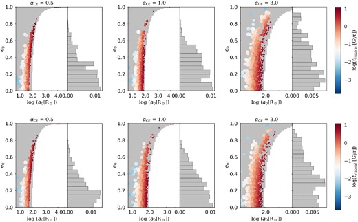
The distribution of the eccentricity versus the orbital semimajor axis at the BBH formation, runs for kickF = k3 and metallicity Z = 0.0002 is shown. The shaded region in each panel represents the area of theoretical parameter space (e0 , a0) which satisfies tinspiral(e0 , a0) ≤ τH, while the colour-coded scatters label the modelled GW190521-like systems with the colours denoting their tinspiral(e0 , a0) values and the size denotes the weight of each system in the population. Columns from left to right correspond to the simulations with αCE = 0.5, 1.0, and 3.0, respectively. The top and bottom panels correspond to ‘ei = 0’ and ‘ei = 0 ∼ 1’ models. The horizontal histograms represent the merger rate density |$\mathcal {R}$|-weighted distribution of e0.
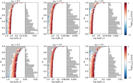
Figs 3–5 show the results of Z = 0.0004, 0.0008, and 0.0016, respectively. They reflect the similar tendency as in Fig. 2. A comparison of Figs 2–5 shows that, as the metallicity increases, there are more BBHs with large eccentric and wide orbits (e0 > 0.8 and a0 > 100 R⊙). This is because the progenitors of GW190521-like system at higher Z are more massive, and thus have larger size than those at low Z.
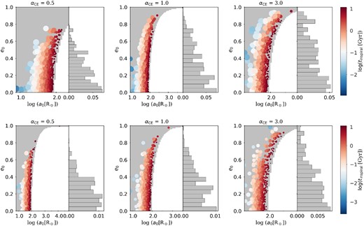
Same as Fig. 2, but for Z = 0.0004.
Same as Fig. 2, but for Z = 0.0008.
Same as Fig. 2, but for Z = 0.0016.
Current and upcoming missions such as the ground-based aLIGO, Cosmic Explorer (Reitze et al. 2019), Einstein telescope (ET; Punturo et al. 2010), and the space-borne DECi-hertz Interferometer Gravitational Wave Observatory (DECIGO; Seto, Kawamura & Nakamura 2001), and Laser Interferometer Space Antenna (LISA; Amaro-Seoane et al. 2017) would detect thousands of merger events of BBHs per year (Evans et al. 2021).We explore whether GW190521-like systems could be detected by these instruments. In Fig. 6, the left three panels present the evolution of the eccentricity of GW190521-like systems during the inspiral prior to merge as a function of the peak frequency. The GW emission dominates the evolution of the binary semimajor axis and eccentricity, leading to efficient circularization of the BBH systems before the merger. The right three panels present the GW signal characteristic strain at the npeakth harmonic along with the orbital evolution as a function of the peak frequency, which is the key ingredient determining whether such mergers can be seen with the GW detectors, in the ‘ei = 0’ model. The evolutionary tracks (calculated with equations 29 and 30) are gradually overlapped by the sensitivity curves of LISA, DECIGO, ET, Cosmic Explorer, A + LIGO, and aLIGO during the orbital shrinking and circularizing stage. The systems become largely circularized before entering the sensitivity band of ET, Cosmic Explorer, A + LIGO, and aLIGO, and any residual eccentricity is expected to have a negligible effect on their detectability (Mandel et al. 2008). The most distant detectable GW190521-like mergers are at the redshfit ∼4.4. Fig. 7 shows the results in the ‘ei = 0 ∼ 1’ model, and there are no significant differences compared with Fig. 6.
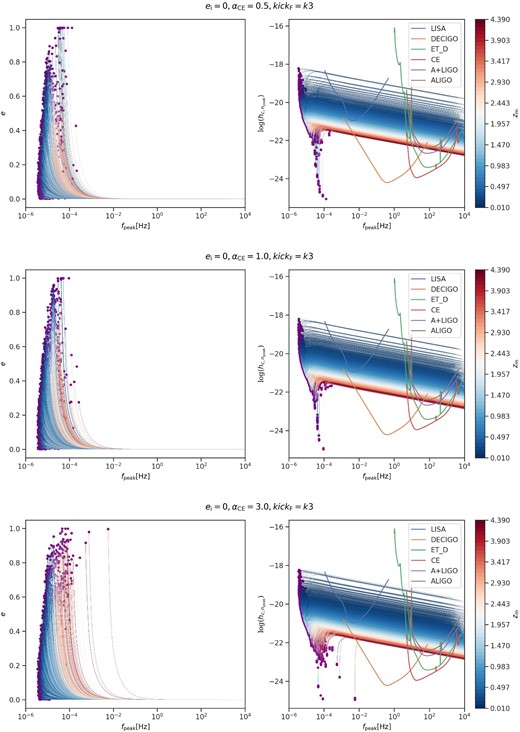
Evolution of the eccentricity (left-hand panels) and the characteristic strain |$h_{\rm c,n_{peak}}$| (right-hand panels) versus the peak frequency fpeak of GW190521-like systems from inspiral to nearly merger (‘ei = 0’ model, kickF = k3). The purple points label the formation of BBHs. From top to bottom are the runs with αCE = 0.5, 1.0, and 3.0, respectively. The colours of the line denote the redshift zm where the merged sources are located. The simulated tracks of the sensitivity curve of space-borne GW detectors LISA (Robson, Cornish & Liu 2019), DECIGO (Yagi & Seto 2011), and the ground-based detectors ET (Hild et al. 2011), Cosmic Explorer (shown as 'CE' in legend) (Abbott et al. 2017b), A + LIGO, and aLIGO (LIGO Document a, b) are also shown.

Same as Fig. 6 but for ‘ei = 0 ∼ 1’ model.
Another important characteristic of merging BBHs is their spins, which get imprinted in the GW signal (Cutler, Flanagan & É. 1994). The BH progenitors gain and lose their spin angular momenta through stellar evolution, mass transfer, and tidal interactions (Hurley et al. 2002; Belczynski et al. 2020b; Tanikawa et al. 2021b). The spin angular momenta are generally parallel to the orbital angular momentum, until the kicks to the BHs cause their spin axes tilted. According to traditional tidal theory (Zahn 1977; Hut 1981), the torque depends on the ratio of the stellar radius R to the separation a of both stars, that is, ∝(R/a)6. Because the progenitor of BH1 is very massive and the initial orbit is very wide, spinning up of the BH1’s progenitor is ineffective, so the merging BBHs generally have small |χeff|. In the ‘ei = 0’ model, χeff = 0 ∼ 0.1 (kickF = k3) and −0.09 ∼ 0.1 (kickF = k1, k2); in the ‘ei = 0 ∼ 1’ model, χeff = −0.08 ∼ 0.1 (kickF = k3) and −0.1 ∼ 0.1 (kickF = k1, k2). They are in contradiction with Nitz & Capano (2021)’s prediction that the BH spin is anti-aligned with the orbital angular momentum and |$\chi _{\rm eff}=-0.51_{-0.11}^{+0.24}$|. However, the mechanism of tidal interactions is not well understood. If we adopt the Geneva model (Eggenberger et al. 2008) in which angular momentum is mainly transported by meridional currents (see also Belczynski et al. 2020a), |$|\overrightarrow{\chi _1}|$| can increase from ∼0 to ∼0.25. As the spin of the merger product is dominated by the contribution of the more massive BH1, the estimated χeff changes to be −0.3 ∼ 0.32. We also note that, by using the Tayler–Spruit magnetic dynamo angular transport, Belczynski et al. (2020a) inferred the natal spins of BBHs (m1 = 84.9 M⊙, m2 = 64.6 M⊙) that would merge within Hubble time to be |$|\overrightarrow{\chi _1}| = 0.052$| and |$|\overrightarrow{\chi _2}| = 0.523$|.
4 DISCUSSION
The natal kick plays a key role in the life of a compact star binary, as it affects not only the orbital parameters and systemic velocity, but also the binary evolutionary path (Brandt & Podsiadlowski 1995). There is a general consensus that NSs are usually born with large kick velocities |$v_{\rm kick,NS}\sim 200{\!-\!}500\, \rm kms^{-1}$| (Lyne & Lorimer 1994). However, the origin of the SN kick is in debate. One possible mechanism is the asymmetric material ejection during the SN explosion, triggered by the large-scale hydrodynamic perturbation or convection instabilities in the SN core (Burrows & Hayes 1996; Goldreich, Lai & Sahrling 1997; Scheck et al. 2004; Nordhaus et al. 2012; Gessner & Janka 2018). Other investigations suggest that it may be related to the anisotropic neutrino emission from the proto-NS induced by strong magnetic field (Kusenko & Segrè 1996; Lai & Qian 1998; Maruyama et al. 2011). Besides, the topological current may be responsible for the natal kick (Charbonneau & Zhitnitsky 2010).
The kick velocity distribution is also in active study. Arzoumanian, Chernoff & Cordes (2002) studied the velocity distribution of radio pulsars based on large-scale 0.4 GHz pulsar surveys, and found a two-component velocity distribution with characteristic velocities of 90 and 500 kms−1. Hobbs et al. (2005) analysed a catalogue of 233 pulsars with proper motion measurements, and suggested the NS natal kick distribution with a Maxwellian one-dimensional dispersion |$\sigma _{\rm NS}=265\, \rm kms^{-1}$|, which is widely used in later studies. From the analysis of the proper motions of 28 pulsars using very long baseline array interferometry data, Verbunt, Igoshev & Cator (2017) showed that a distribution with two Maxwellians improves significantly on a single Maxwellian for the young pulsar velocities.
Whether stellar-mass BHs receive such large kicks is also a matter of debate. A growing number of studies have been devoted to investigate the natal kicks of BHs relying on a variety of methods and data sets, such as the study of massive runaway and walkaway stars (Blaauw 1961; De Donder, Vanbeveren & van Bever 1997; Renzo et al. 2019; Aghakhanloo et al. 2022), BH X-ray binaries (Mirabel et al. 2001; Jonker & Nelemans 2004; Repetto et al. 2012; Wong et al. 2012, 2014; Atri et al. 2019; Kimball et al. 2022), astrometric microlensing (Andrews & Kalogera 2022), and merging BBH GW events (Abbott et al. 2021; The LIGO Scientific Collaboration 2021).
In light of the observational constraints on the NS/BH natal kick velocities, several phenomenological and analytical kick prescriptions are proposed, mainly depending on the SN ejecta mass and remnant mass (e.g. Bray & Eldridge 2018; Giacobbo & Mapelli 2020; Mandel & Müller 2020; Richards et al. 2023). Because the kick-induced orbital eccentricity determines the time-scale over which BBHs are expected to merger via GW radiation, the merging history of BBHs provide a probe to the natal kick received by BHs. Based on the premise that GW190521 is an IMRI with component masses of |${\sim} 170$| and |${\sim} 16\, {\rm M}_{\odot }$| (Nitz & Capano 2021), we examine the isolated binary evolution channel with three kick prescriptions. In the k1 and k2 prescriptions, the BH natal kick is determined by the fallback fraction ffb so massive BH experienced totally fallback (ffb = 1.0) would receive no kick, while in k3 prescription BHs always receive a kick produced through asymmetric neutrino emission.
Our calculations indicate that, to produce the merger event, the less massive BH should receive a natal kick with velocity of a few hundred |$\rm kms^{-1}$|, thus preferring the k3 prescription. This is of particular interest since in most cases both BHs formed through totally fallback, and the conclusion is not sensitive to the choice of the CE efficiency αCE.
We predict the merger rate density of GW190521-like systems |$\mathcal {R}(z\le 1.1)\sim 4\times 10^{-5}{\!-\!}5\times 10^{-2} \, \rm Gpc^{-3}yr^{-1}$| if the BH natal kick is weighted to follow a Maxwell distribution of the NS kick with σNS = 265 kms−1. Under the interpretation that GW190521 is an almost equal mass ratio system, LIGO/Virgo collaboration reported the merger rate density of GW190521-like systems to be |$0.13_{-0.11}^{+0.30}\, \rm Gpc^{-3} yr^{-1}$| with the effective spin parameter |$\chi _{\rm eff}=0.08_{-0.36}^{+0.27}$| (Abbott et al. 2020a, b). By employing a new estimate of the PPISN mass-loss, Belczynski et al. (2020a) obtained a merger rate density of |${\sim} 0.04\, \rm Gpc^{-3} yr^{-1}$| for such events via isolated binary evolution. Tanikawa et al. (2021b) estimated the merger rate density of Population III BBHs (with total mass |${0\sim} 130{\!-\!}260\, {\rm M}_{\odot }$| and composing at least one |$130{\!-\!}200\, {\rm M}_{\odot }$| IMBH) about 0.01 |$\rm Gpc^{-3}yr^{-1}$|. Hijikawa et al. (2022) performed a BPS calculation for very massive Population III stars and derived the property of the BBH mergers, adopting constant values for αCEλ in their CE evolution. In their ‘low mass + high mass’ model, the resultant compact binaries consist of a stellar mass BH (below the PISN mass gap) and an IMBH (above the PISN mass gap) with mass ratio ranging from 0.15 to 0.35. The predicted merger rate density peaks at z ∼ 10 with a value of |$(1-10)\, \rm Gpc^{-3}yr^{-1}$|, and declines to nearly zero at z ≤ 3 because of the very short delay time (less than 10 |$\rm Myr$|). In our Population II evolution channel, the merger rate peaks at z ∼ 2 with the delay time ranging from |${\sim} 1.4{\!-\!}12.1\, \rm Gyr$|.
5 SUMMARY
The third observing run operated by aLIGO and advanced Virgo discovered a massive BBH merger event GW190521, with a remnant total mass of |$150_{{-17}}^{+29}\, {\rm M}_{\odot }$|, falling in the IMBH regime (Abbott et al. 2020a), and the component masses were estimated to be |$(m1, m2) = (85_{{-14}}^{+21}$|, |$66_{{-18}}^{+17})\, {\rm M}_{\odot }$| within 90 per cent credible region (see also Barrera & Bartos 2022; Gamba et al. 2023). Nitz & Capano (2021), however showed that GW190521 may be alternatively an IMRI, with the component masses of m1 ∼ 170 M⊙ and m2 ∼ 16 M⊙, which happen to straddle the PISN mass gap. In the most recent analysis, Gamba et al. (2023) revealed the BH masses to be |$81_{{-25}}^{+62}\, {\rm M}_{\odot }$| and |$52_{{-32}}^{+32}\, {\rm M}_{\odot }$| under the hypothesis that it was generated by the merger of two non-spinning BHs on hyperbolic orbits. So, the nature of GW190521 is still uncertain.
Assuming the configuration of Nitz & Capano (2021) for GW190521 (or similar systems to be discovered in the future), we perform BPS simulation to interpret the formation of GW190521-like systems via isolated binary evolution channel. Our analyses prefer that this merger event had evolved from primordial binary systems in metal-poor environment with Z ≤ 0.0016. The majority of them are formed via an initial phase of stable RLOF before the formation of the BH1, followed by a CE phase triggered by collision at periastron when BH1’s companion is a giant-like star in a close eccentric orbit. The initial ZAMS progenitor masses are expected to be |$M_{\rm i,1}\sim 300{\!-\!}800\, \rm {\rm M}_{\odot }$| and |$M_{\rm i,2}\sim 20{\!-\!}60\, {\rm M}_{\odot }$|, respectively, which are metallicity-dependent. By using the fallback independent kick prescription, the merger event requires the primary and secondary BHs to receive natal kicks with velocities |$v_{\rm kick,1}\ \lt\ 50\, \rm kms^{-1}$| and |$v_{\rm kick,2} \ \lt\ 700\, \rm kms^{-1}$|. Our results support the hypothesis that BHs formed by direct core collapse receive considerable large natal kick. The predicted merger rate density for GW190521-like systems is |$4\times 10^{-5}{\!-\!}5\times 10^{-2} \, \rm Gpc^{-3}yr^{-1}$| at zm ≤ 1.1. We also find that, using the traditional treatment of tidal interaction results in very small effective spin parameter, but if using the Geneva model instead, χeff ranges from −0.3 to 0.32, roughly located within the interval |$-0.51^{-0.11}_{+0.24}$| estimated by Nitz & Capano (2021).
ACKNOWLEDGEMENTS
We thank the anonymous referee for useful comments, which helped improve the manuscript. We are also grateful to Shi-Jie Gao for help with the calculation of λ. This work was supported by the Natural Science Foundation of China under grant no. 12041301and12121003, and the National Key Research and Development Program of China (grant no. 2021YFA0718500). We acknowledge use of the following python packages: astropy (Astropy Collaboration 2013), matplotlib (Hunter 2007), numpy (van der Walt, Colbert & Varoquaux 2011), and scipy (Virtanen et al. 2020).
DATA AVAILABILITY
All data underlying this article will be shared on reasonable request to the corresponding authors.
Footnotes
The baryonic mass is reduced by the neutrinos that are lost (Burrows & Lattimer 1986), and we assume that for BHs the gravitational mass MBH is |$99{{\ \rm per\ cent}}$| of the baryonic mass MBH,bar for our considered massive BBHs.
Belczynski et al. (2020a) recently suggested that if the 12C(α, γ)O16 reaction rate is 3σ lower than its standard rate, star with Helium core mass MHe ∼ 90 M⊙ can avoid PISN and evolve to a mass gap BH.
References
APPENDIX A: THE CE PARAMETER λ FOR VERY MASSIVE STARS
In our stellar models, we neglect any stellar rotation. For stellar winds, we use the Vink et al. wind prescription as mentioned in Section 2.1, but the result in Nugis & Lamers (2000) for Wolf–Rayet stars. The convective regions are determined by the Schwarzschild criterion using αMLT = 1.73 (MacLeod et al. 2017), and we assume an exponential overshoot (Herwig 2000) by 1 per cent of the scale height.
Figs A1 and A2 show the evolution of λb(the thick solid lines) and λg(the thin solid lines) with stellar radius for different masses at Z = 0.02, 0.001, and 0.0001. We make polynomial fitting of the results with
where R is the stellar radius. Tables A1 and A2 provide the coefficients ni(i = 0, 10) for stars with selected masses. The goodness of fit χ2 ≃ 0.998.
Evolution of binding energy parameter λb (the thick solid lines) and λg (the thin solid lines) vary with stellar radius for different massive stars. Results with Z = 0.02 (the left-hand panel), Z = 0.001 (the middle panel), and Z = 0.0001 (the right-hand panel). Models with M = 20, 40, and 60 M⊙ at Z = 0.02 in Wang et al. (2016) and M = 20 M⊙ at Z = 0.001 in Xu & Li (2010) are also shown with dashed lines as controls.
Same as Fig. A1 but for more massive stars.
Fitting coefficients for λb.
| λ | Mass (M⊙) | n0 | n1 | n2 | n3 | n4 | n5 | n6 | n7 | n8 | n9 | n10 |
|---|---|---|---|---|---|---|---|---|---|---|---|---|
| Z = 0.02 | ||||||||||||
| 40 | 0.5435 | −0.031 84 | 0.000 2715 | −1.227e-06 | 3.209e-09 | −5.196e-12 | 5.375e-15 | −3.56e-18 | 1.461e-21 | −3.382e-25 | 3.378e-29 | |
| 60 | 0.6051 | −0.025 82 | 0.000 1443 | −4.475e-07 | 8.257e-10 | −9.575e-13 | 7.162e-16 | −3.451e-19 | 1.034e-22 | −1.754e-26 | 1.286e-30 | |
| 80 | 0.6566 | −0.022 67 | 9.957e-05 | −2.494e-07 | 3.81e-10 | −3.721e-13 | 2.367e-16 | −9.745e-20 | 2.498e-23 | −3.616e-27 | 2.254e-31 | |
| 100 | 0.6693 | −0.018 09 | 5.575e-05 | −9.112e-08 | 7.847e-11 | −2.704e-14 | −9.748e-18 | 1.372e-20 | −5.748e-24 | 1.129e-27 | −8.781e-32 | |
| 130 | 0.5937 | −0.011 64 | 3.108e-05 | −6.794e-08 | 1.096e-10 | −1.178e-13 | 8.156e-17 | −3.571e-20 | 9.536e-24 | −1.416e-27 | 8.955e-32 | |
| Z = 0.001 | ||||||||||||
| 40 | 0.5478 | −0.0358 | 0.000 4194 | −2.648e-06 | 9.582e-09 | −2.114e-11 | 2.94e-14 | −2.588e-17 | 1.398e-20 | −4.228e-24 | 5.482e-28 | |
| 60 | 0.6674 | −0.033 72 | 0.000 2993 | −1.399e-06 | 3.726e-09 | −6.048e-12 | 6.193e-15 | −4.02e-18 | 1.604e-21 | −3.588e-25 | 3.446e-29 | |
| 80 | 0.7491 | −0.031 38 | 0.000 2319 | −8.724e-07 | 1.845e-09 | −2.363e-12 | 1.906e-15 | −9.73e-19 | 3.053e-22 | −5.37e-26 | 4.055e-30 | |
| 100 | 0.7908 | −0.028 09 | 0.000 1731 | −5.611e-07 | 1.05e-09 | −1.213e-12 | 8.937e-16 | −4.206e-19 | 1.225e-22 | −2.009e-26 | 1.421e-30 | |
| 150 | 0.6241 | −0.009 325 | −1.416e-05 | 1.386e-07 | −2.997e-10 | 3.234e-13 | −2.025e-16 | 7.697e-20 | −1.753e-23 | 2.203e-27 | −1.175e-31 | |
| 200 | 0.7362 | −0.011 71 | 2.096e-05 | −1.864e-08 | 9.033e-12 | −2.438e-15 | 3.444e-19 | −1.986e-23 | – | – | – | |
| 250 | 0.7734 | −0.010 13 | 1.674e-05 | −8.327e-09 | −8.46e-12 | 1.412e-14 | −8.661e-18 | 2.889e-21 | −5.523e-25 | 5.694e-29 | −2.46e-33 | |
| 300 | 0.8114 | −0.009 691 | 1.45e-05 | −1.085e-08 | 4.247e-12 | −8.348e-16 | 6.517e-20 | – | – | – | – | |
| Z = 0.0001 | ||||||||||||
| 40 | 0.3171 | −0.016 58 | 6.395e-05 | −1.197e-07 | 1.126e-10 | −5.171e-14 | 9.225e-18 | – | – | – | – | |
| 60 | 0.4729 | −0.028 87 | 0.000 2611 | −1.259e-06 | 3.443e-09 | −5.681e-12 | 5.86e-15 | −3.803e-18 | 1.508e-21 | −3.338e-25 | 3.161e-29 | |
| 80 | 0.7627 | −0.037 71 | 0.000 268 | −9.484e-07 | 1.87e-09 | −2.22e-12 | 1.649e-15 | −7.712e-19 | 2.207e-22 | −3.528e-26 | 2.414e-30 | |
| 100 | 0.6976 | −0.026 94 | 0.000 1746 | −5.963e-07 | 1.16e-09 | −1.371e-12 | 1.02e-15 | −4.795e-19 | 1.382e-22 | −2.229e-26 | 1.54e-30 | |
| 150 | 0.6742 | −0.016 49 | 5.084e-05 | −7.856e-08 | 6.492e-11 | −2.924e-14 | 6.767e-18 | −6.291e-22 | – | – | – | |
| 200 | 0.7422 | −0.015 26 | 4.124e-05 | −4.653e-08 | 7.804e-12 | 3.139e-14 | −3.343e-17 | 1.61e-20 | −4.216e-24 | 5.817e-28 | −3.318e-32 | |
| 250 | 0.516 | −0.002 953 | 1.331e-06 | −2.585e-10 | 1.748e-14 | – | – | – | – | – | – | |
| 300 | 0.8598 | −0.0158 | 4.625e-05 | −6.992e-08 | 5.992e-11 | −3.098e-14 | 9.893e-18 | −1.925e-21 | 2.14e-25 | −1.141e-29 | 1.573e-34 |
Same as Table A1 but for λg.
| λ | Mass (M⊙) | n0 | n1 | n2 | n3 | n4 | n5 | n6 | n7 | n8 | n9 | n10 |
|---|---|---|---|---|---|---|---|---|---|---|---|---|
| Z = 0.02 | ||||||||||||
| 40 | 0.144 | −0.036 83 | 0.000 3541 | −1.767e-06 | 5.024e-09 | −8.734e-12 | 9.615e-15 | −6.731e-18 | 2.903e-21 | −7.036e-25 | 7.33e-29 | |
| 60 | 0.03541 | −0.022 24 | 0.000 1293 | −4.263e-07 | 8.269e-10 | −9.924e-13 | 7.581e-16 | −3.693e-19 | 1.111e-22 | −1.882e-26 | 1.373e-30 | |
| 80 | −0.05606 | −0.014 11 | 3.883e-05 | −4.339e-08 | −1.224e-11 | 8.372e-14 | −9.515e-17 | 5.486e-20 | −1.774e-23 | 3.062e-27 | −2.203e-31 | |
| 100 | 0.03445 | −0.016 07 | 5.61e-05 | −1.16e-07 | 1.474e-10 | −1.183e-13 | 6.02e-17 | −1.896e-20 | 3.461e-24 | −3.122e-28 | 8.471e-33 | |
| 130 | 0.01228 | −0.014 78 | 7.119e-05 | −2.132e-07 | 3.702e-10 | −3.893e-13 | 2.564e-16 | −1.065e-19 | 2.712e-23 | −3.869e-27 | 2.368e-31 | |
| Z = 0.001 | ||||||||||||
| 40 | 0.070 05 | −0.034 53 | 0.000 3868 | −2.385e-06 | 8.509e-09 | −1.861e-11 | 2.574e-14 | −2.258e-17 | 1.217e-20 | −3.675e-24 | 4.76e-28 | |
| 60 | 0.083 48 | −0.029 32 | 0.000 2426 | −1.088e-06 | 2.807e-09 | −4.432e-12 | 4.425e-15 | −2.802e-18 | 1.091e-21 | −2.382e-25 | 2.231e-29 | |
| 80 | 0.096 17 | −0.026 41 | 0.000 1841 | −6.737e-07 | 1.4e-09 | −1.769e-12 | 1.41e-15 | −7.117e-19 | 2.208e-22 | −3.839e-26 | 2.864e-30 | |
| 100 | 0.103 | −0.024 12 | 0.000 1445 | −4.624e-07 | 8.514e-10 | −9.62e-13 | 6.891e-16 | −3.14e-19 | 8.821e-23 | −1.393e-26 | 9.459e-31 | |
| 150 | 0.1182 | −0.020 12 | 0.000 1171 | −3.371e-07 | 5.206e-10 | −4.745e-13 | 2.686e-16 | −9.566e-20 | 2.088e-23 | −2.555e-27 | 1.342e-31 | |
| 200 | 0.1519 | −0.0191 | 9.396e-05 | −2.224e-07 | 2.831e-10 | −2.134e-13 | 1.003e-16 | −2.972e-20 | 5.408e-24 | −5.52e-28 | 2.422e-32 | |
| 250 | 0.1054 | −0.015 21 | 6.26e-05 | −1.315e-07 | 1.512e-10 | −1.037e-13 | 4.446e-17 | −1.203e-20 | 1.999e-24 | −1.863e-28 | 7.466e-33 | |
| 300 | 0.1743 | −0.017 09 | 8.94e-05 | −2.608e-07 | 4.266e-10 | −4.174e-13 | 2.544e-16 | −9.753e-20 | 2.287e-23 | −2.997e-27 | 1.683e-31 | |
| Z = 0.0001 | ||||||||||||
| 40 | −0.1711 | −0.015 38 | 5.801e-05 | −1.069e-07 | 9.934e-11 | −4.504e-14 | 7.935e-18 | – | – | – | – | |
| 60 | −0.044 46 | −0.027 63 | 0.0002392 | −1.129e-06 | 3.042e-09 | −4.968e-12 | 5.082e-15 | −3.275e-18 | 1.291e-21 | −2.845e-25 | 2.684e-29 | |
| 80 | 0.043 96 | −0.025 77 | 0.0001593 | −5.317e-07 | 1.025e-09 | −1.21e-12 | 9.021e-16 | −4.257e-19 | 1.232e-22 | −1.992e-26 | 1.379e-30 | |
| 100 | −0.0111 | −0.021 01 | 0.0001237 | −4.057e-07 | 7.76e-10 | −9.134e-13 | 6.808e-16 | −3.218e-19 | 9.345e-23 | −1.52e-26 | 1.059e-30 | |
| 150 | 0.0299 | −0.017 25 | 8.402e-05 | −2.49e-07 | 4.516e-10 | −5.153e-13 | 3.758e-16 | −1.745e-19 | 4.979e-23 | −7.951e-27 | 5.435e-31 | |
| 200 | 0.039 78 | −0.014 77 | 5.592e-05 | −1.205e-07 | 1.543e-10 | −1.235e-13 | 6.328e-17 | −2.079e-20 | 4.236e-24 | −4.876e-28 | 2.426e-32 | |
| 250 | −0.088 52 | −0.008 596 | 1.748e-05 | −1.76e-08 | 9.417e-12 | −2.746e-15 | 4.127e-19 | −2.503e-23 | – | – | – | |
| 300 | 0.073 19 | −0.014 25 | 4.956e-05 | −9.459e-08 | 1.05e-10 | −7.172e-14 | 3.104e-17 | −8.531e-21 | 1.441e-24 | −1.365e-28 | 5.542e-33 |
