


ABSTRACT
Star formation is a complex process that typically occurs in dense regions of molecular clouds mainly regulated by magnetic fields, magnetohydrodynamic (MHD) turbulence, and self-gravity. However, it remains a challenging endeavour to trace the magnetic field and determine regions of gravitational collapse, where the star is forming. Based on the anisotropic properties of MHD turbulence, a new technique termed velocity gradient technique (VGT) has been proposed to address these challenges. In this study, we apply the VGT to two regions of the giant California Molecular Cloud (CMC), namely, L1478 and L1482, and analyse the difference in their physical properties. We use the 12CO (J = 2–1), 13CO (J = 2–1), and C18O (J = 2–1) emission lines observed with the Heinrich Hertz Submillimeter Telescope. We compare VGT results calculated in the resolutions of 3.3 and 10 arcmin to Planck polarization at 353 GHz and 10 arcmin to determine areas of MHD turbulence dominance and self-gravity dominance. We show that the resolution difference can introduce misalignment between the two measurements. We find the VGT-measured magnetic fields globally agree with those from Planck in L1478, suggesting self-gravity’s effect is insignificant. The best agreement appears in VGT-12CO. As for L1482, the VGT measurements are statistically perpendicular to the Planck polarization indicating the dominance of self-gravity. This perpendicular alignment is more significant in VGT-13CO and VGT-C18O.
1 INTRODUCTION
Magnetic field and turbulence are pervasive in the interstellar medium (ISM; Armstrong, Rickett & Spangler 1995; Chepurnov & Lazarian 2010; Crutcher 2012; Berdyugin, Piirola & Teerikorpi 2014; Han 2017; Hu, Yuen & Lazarian 2020a; Hu, Lazarian & Wang 2022a). They play a vital role in many astrophysical processes including star formation, molecular cloud evolution (Crutcher 2004; Mac Low & Klessen 2004; McKee & Ostriker 2007; Federrath & Klessen 2012; Lazarian, Esquivel & Crutcher 2012), cosmic ray propagation (Jokipii 1966; Ghilea et al. 2011; Xu & Yan 2013; Shukurov et al. 2017; Xu 2022; Hu, Lazarian & Xu 2022b), and solar flares (Moore et al. 2001; Judge et al. 2021; Pontin & Priest 2022). Nevertheless, magnetic field’s role in molecular cloud evolution and star formation is hotly debated, mostly due to the insufficient information on magnetic field structure and strength. Specifically, magnetic fields are challenging to trace and map. Identifying regions where gravity takes over and distinguishing them from regions, where gravity is successfully counteracted by the magnetic field and turbulence remain another obscured (Crutcher 2012).
Important efforts to map magnetic fields have been utilized, including dust polarization from background starlight (Heiles 2000; Berdyugin et al. 2014) or polarized thermal dust emission (Andersson, Lazarian & Vaillancourt 2015; Planck Collaboration: et al. 2015; Chuss et al. 2019; Hwang et al. 2021; Tram et al. 2023). These are widely used to trace the plane-of-the-sky (POS) magnetic field orientation in molecular clouds. Zeeman Splitting (Crutcher 2004, 2012) and Faraday rotation (Tahani et al. 2019, 2022), on the other hand, can measure the magnetic field strength along the line of sight (LOS). In terms of the POS magnetic field, polarization measurements have considerably advanced our knowledge of the magnetic field in molecular clouds. Nevertheless, adequate knowledge of the POS magnetic field’s variation along the LOS or as a function of gas volume density is still missing. The latter is particularly crucial in understanding star formation as the self-gravity’s significance increases in dense regions, and it is important to understand at which densities the gravity takes control of the gas dynamics (Crutcher 2012; Xu & Lazarian 2020; Hu, Lazarian & Yuen 2020b).
To access the POS magnetic field’s variation relative to gas density, we employ the novel Velocity Gradient Technique (VGT; González-Casanova & Lazarian 2017; Yuen & Lazarian 2017; Hu, Yuen & Lazarian 2018; Lazarian & Yuen 2018) to trace the magnetic field’s orientation within molecular clouds. VGT works by utilizing the anisotropy of magnetohydrodynamic (MHD) turbulence (Goldreich & Sridhar 1995), which, together with the turbulent reconnection (Lazarian & Vishniac 1999), makes turbulent eddies aligned and elongated along the direction of the magnetic field that percolates the eddies. Such eddies induce velocity fluctuations that are maximal in the direction perpendicular to the magnetic field at the position of these eddies, a fact supported by numerous simulations (Cho & Vishniac 2000; Cho & Lazarian 2003; Hu, Xu & Lazarian 2021a). Consequently, the gradient of velocity fluctuations is maximal when perpendicular to the magnetic field component, revealing this component.
The turbulence’s property, i.e. velocity fluctuation, can be accessed via the Doppler-shifted spectroscopic emission line. Particularly, the emission lines from different molecular species arise at different optical depths, corresponding to different gas densities. For instance, 12CO typically traces the volume density1 around 102 cm−3, while denser C18O traces the density roughly around 104 cm−3. Applying VGT to various emission lines, therefore, can reveal the magnetic field’s variation from diffuse regions to dense regions. This method has been applied with success to multiple different molecular clouds (Hu et al. 2019a; Hu, Lazarian & Xu 2021c; Alina et al. 2022; Liu, Hu & Lazarian 2022; Zhao et al. 2022).
The direction of velocity gradients changes in the regions of gravitational collapse. Thus, VGT can reveal the relative importance of MHD turbulence and self-gravity. Simulations (Lazarian & Yuen 2018; Hu et al. 2020b) testify that when self-gravity dominates over turbulence, the velocity gradients are dominated by the inward collapse parallel to the magnetic field. This change is characterized by a shift in the cloud dynamics where the VGT orientation flips by at most 90° to align parallel with the magnetic field inferred from polarization (Hu et al. 2020b). Such a change of direction observed in a given emission line suggests the volume density threshold that can trigger gravitational collapse.
The VGT has been proven to be a reliable tool for tracing the magnetic field in diffuse media and in clouds with low star formation rates (Lu, Lazarian & Pogosyan 2020; Hu et al. 2020b; Hu, Lazarian & Stanimirović 2021b). In this study, we explore the performance of VGT in massive star-forming regions. For our research, we chose to study the L1478 and L1482 star-forming regions of the California molecular cloud (CMC), which is roughly 450 pc (Lada, Lombardi & Alves 2009) away from Earth. L1478 and L1482 are both chosen for their distinguishable properties. Although, they are two neighbouring filamentary regions, their orientation relative to the Galactic plane is different, i.e. L1478 orientates to the north-west while L1482 is to the north-east (Lewis et al. 2021). Particularly, L1478 has a lower column density and is more diffuse than L1482, suggesting the significance of self-gravity within the two regions might be different (Chung et al. 2019). These facts make these two regions prime targets for studying the magnetic field and self-gravity’s effects on the molecular cloud’s evolution through VGT.
In order to calculate the velocity gradient, we used 12CO (J = 2–1), 13CO (J = 2–1), and C18O (J = 2–1) spectral lines observed with the Heinrich Hertz Submillimeter Telescope (SMT; Lewis et al. 2021). These three molecules exhibit different optical depths and are sensitive to different density ranges. 12CO typically optically thick (optical depths ≫1), tracing the cloud’s outskirt diffuse region, while C18O is optically thin (optical depths ≪1), imprinting the information of the cloud’s dense core (Hu et al. 2019b; Lewis et al. 2021). This fact allows us to form a 3D magnetic field tomography within the molecular cloud along the LOS utilizing VGT. Additionally, to investigate the significance of self-gravity, we compare the VGT-derived magnetic fields with the one inferred from the Planck dust polarization at 353 GHz (Planck Collaboration et al. 2020).
In this research, we measure the magnetic field of L1478 and L1482 regions of the California molecular cloud with the VGT method. This paper is organized into six sections. In Section 2, we describe the observational data that was used for this research. In Section 3, we introduce the methodology behind VGT and its established pipeline. In Section 4, we present our observational results of magnetic fields traced by VGT using different tracers and then compare our results with Planck polarization results. In Section 5, we discuss the importance of VGT and its applicability. We also discuss its agreement and anti-agreement with Planck polarization and its physical implications for the CMC. Finally, in Section 6, we conclude with a summary of our work.
2 OBSERVATIONAL DATA
2.1 Emission line
We used data from Lewis et al. (2021) who observed 12CO (J = 2–1), 13CO (J = 2–1), and C18O (J = 2–1) spectral line measurements of L1478 and L1482 from the SMT using a prototype ALMA Band 6 dual-polarization sideband separating receiver in combination with the 0.25 MHz–256 channel filterbank as the back end (0.25 MHz ∼0.32 km s−1 at 230 GHz). The beam and velocity resolution for each CO tracer were slightly different, the maps were therefore convolved to the same resolution of the 12CO (38 arcmin) and regridded into pixel resolution of 10 arcmin and velocity resolution to 0.3 km s−1 to allow for comparison. As for noise level, the average rms noise per 0.3 km s−1 channel was 0.005 K for C18O, 0.03 K for 13CO, and 0.07 K for 12CO. The averaged spectrum for each line is presented in Appendix B.
To derive the column density map, we adopt the X-factor method used in Pineda, Caselli & Goodman (2008). The X-factor of 12CO, i.e. X12 is defined as:
where W12 is the integrated 12CO intensity and |$N_{\rm H_2}$| is the column density map. For simplicity, we use a uniform value X12 = 2 × 1020 cm−2 K−1 km−1 s (Pineda et al. 2008). To derive column densities from the 13CO and C18O intensity maps, we follow (Pineda et al. 2008):
where Av is the extinction. W13 and W18 are integrated 13CO and C18O intensities, respectively.
2.2 Planck polarization
In our research, we compared the magnetic field inferred from velocity gradient to the one obtained from Planck polarization data (Planck Collaboration et al. 2020). We use the Planck 353 GHz polarized dust signal data from the Planck 3rd Public Data Release (DR3) 2018 of High Frequency Instrument. Observations from Planck designate the polarization angle ϕ with Stokes parameter maps I, Q, and U. ϕ is defined mathematically as:
where the −U notation converts the angle from HEALPix convention to IAU convention. The Stokes parameter maps were smoothed from nominal angular resolution 5–10 arcmin with a Gaussian kernel to suppress noise and achieve a higher sign-to-noise ratio. We infer the magnetic field angle from the equation: ϕB = ϕ + |$\pi$|/2.
Note that the foreground contribution is not calibrated in the Planck data. L1478 and L1482 are nearby clouds with an infrared extinction derived from Herschel’s observations 1.5–4 (Lada et al. 2017). The extinction is much larger than that of the diffuse foreground. We, therefore, expect the Planck polarization to be dominated by the signal from the clouds.
3 METHODOLOGY
3.1 Basics of VGT
VGT is theoretically based on the theories of MHD turbulence (Goldreich & Sridhar 1995) and fast turbulent reconnection (Lazarian & Vishniac 1999). It has been applied to study magnetic fields in both diffuse and molecular species (Lu et al. 2020; Hu et al. 2020b, 2021b, 2022a; Tram et al. 2023).
The scale-dependent anisotropy of magnetic fluctuations was predicted in Goldreich & Sridhar (1995):
where k⊥ and k∥ are wavevectors perpendicular and parallel to magnetic field. In the original study, the magnetic field was the mean magnetic field. It is important to mention that in Fourier space, the local spatial information is not available so that the anisotropy is measured with respect to the mean magnetic field. This anisotropy in fact is dominated by the largest eddy and is scale-independent (Cho & Vishniac 2000; Hu et al. 2021a).
Nevertheless, turbulent reconnection predicts the existence of eddies that reconnect over the eddy turnover time. Therefore, the magnetic field does not impede the evolution of such eddies and most energy of the cascade is channeled to them. However, it is obvious that the eddies can feel only the magnetic field around them. Thus the parallel and perpendicular scales of eddies l∥ and l⊥ should be identified in terms of the local direction of magnetic field. In these variables, the modified critical balance condition means that the eddy cascading time (l⊥/vl) equals the wave period (l∥/vA), where vA is the Alfvén velocity and vl is turbulent velocity at the perpendicular scale l⊥. According to Lazarian & Vishniac (1999), turbulent eddies, due to the fast magnetic reconnection, mix up the magnetic field in perpendicular direction. The cascade follows the Kolmogorov scaling |$v_{l,\bot }\propto l_{\bot }^{1/3}$|. Consequently, one can get the relation between the parallel and perpendicular scales of the eddies in the local reference frame (i.e. defined by local magnetic fields, see Lazarian & Vishniac 1999):
where Linj is the injection scale and MA = vinj/vA is the Alfvén Mach number, vinj is turbulence’s injection velocity.
Particularly, due to the anisotropy l⊥ ≪ l∥, the amplitude of velocity fluctuation and its corresponding gradient are (Lazarian & Vishniac 1999):
which reveal that the velocity gradient ∇vl is dominated by its perpendicular component and can trace the 3D direction of magnetic field. Note that the anisotropy appears when the local magnetic field’s role is at least comparable to turbulence, i.e. MHD turbulence. For the MA ≫ 1 case, turbulence is isotropic because it is essentially hydrodynamic turbulence. However, the significance of turbulence is cascading from large injection scales (Linj ∼ 100 pc, see Chepurnov & Lazarian 2010) to smaller scales, which means the turbulent velocity decreases. Eventually, at the transition scale |$l_{\rm a} = L_{\rm inj}/M_{\rm A}^3$|, magnetic field and turbulence are comparable (Lazarian 2006). For L1478 and L1482, their length size on the POS is around 5 pc. Therefore, if we consider la < 5 pc, the cloud is in the condition of MA > 3. The typical value for diffuse molecular clouds, however, are sub-Alfvénic MA < 1 or trans-Alfvénic MA ≈ 1 (Pattle et al. 2022). We therefore expect turbulence in L1478 and L1482 to be anisotropic.
The above consideration is valid for MHD turbulence in diffuse ISM, where self-gravity can be ignored. In star forming regions, self-gravity might be significant and dominate over MHD turbulence. In the case of gravitational collapse, i.e. strong self-gravity, the nature of turbulent flow is modified. In the direction perpendicular to the magnetic field, any gravitational pull is counteracted by a magnetic force. The most significant acceleration of the plasma therefore appears in the direction parallel to the magnetic field. The acceleration results in huge velocity difference along the magnetic field so that the velocity gradients are expected to change their orientation from perpendicular to magnetic fields to align with magnetic filed. This property has been numerically and observationally confirmed serving as an important tool in identifying gravitational collapse (Hu et al. 2020b, 2021b).
3.2 VGT pipeline
To extract the velocity information in observation, in this research, we use the thin velocity channel Ch(x, y) of emission lines Lazarian & Yuen (2018). The theory of the fluctuations in such channels is formulated in Lazarian & Pogosyan (2000). According to the theory, narrower the channel width, more significant the contribution of velocity fluctuations. For the density spectrum dominated by large-scale velocity fluctuations, if the channel width Δv is smaller than the velocity dispersion |$\sqrt{\delta (v^2)}$| of turbulent eddies under study, i.e. |$\Delta v < \sqrt{\delta (v^2)}$|, the intensity fluctuation in a thin channel is dominated by velocity fluctuation. Otherwise, the intensity fluctuation is dominated by density fluctuation in a thick channel. Therefore, the intensity gradient calculated in a thin velocity channel map, referred as velocity channel gradients (VChGs) contains the information of velocity fluctuation (Lazarian & Yuen 2018).
Explicitly, the gradient map ψg can be calculated using these equations:
where ∇xChi(x, y) and ∇yChi(x, y) represent the x and y components of the gradient, respectively. The subscript i = 1, 2, …, nv stands for the ith channel map with total number nv. These equations are applied to all pixels with spectral line emissions having a signal-to-noise ratio greater than 3.
The gradient orientation given in equation (7) for each pixel, however, is not statistically sufficient to derive turbulence’s property. The gradient map ψg is further processed by the sub-block averaging method (Yuen & Lazarian 2017) to extract turbulence’s anisotropy. This method takes all velocity gradient orientations within a specific sub-block and plots a corresponding histogram. A Gaussian fitting is applied to the histogram, and the gradient orientation corresponding to Gaussian distribution’s peak value is taken as the mean gradient for that sub-block (see Fig. C1). We denoted the processed gradient map as |$\psi^{i}_{\rm gs}(x,y)$|. The map’s edges with pixel numbers less than the sub-blocks size are not considered in the calculation.
To compare with polarization measurement, we construct the Pseudo-Stokes-parameters Qg and Ug from |$\psi ^{i}_{\rm gs}(x,y)$|:
where ψg is the pseudo polarization angle, which is perpendicular to the POS magnetic field. The magnetic field orientation is then inferred from
Note, ψB is defined as east through the north, while ϕB (from Planck polarization) is defined as north through the west. We transform the Planck angle to VGT’s angle coordinate for comparison.
The alignment between the VGT measurement and polarization measurement is quantified by the Alignment Measure (AM; González-Casanova & Lazarian 2017), defined as:
where θr is the relative angle between the two angles. AM is a relative scale ranging from −1 to 1, with AM = 1 indicating that two angles are parallel, i.e. turbulence dominated and AM = −1 denoting that the two are orthogonal, i.e. self-gravity dominated. The averaged AM values for L1478 and L1482 at resolutions 10 and 3.3 arcmin are listed in Table 1.
This table displays the mean AM values for the corresponding 60 × 60 (i.e. AM60) or 20 × 20 (i.e. AM20) sub-block sizes with corresponding standard deviations for both L1478 and L1482 regions of the CMC. Their corresponding uncertainties |$\sigma _{\rm AM_{60}}$| and |$\sigma _{\rm AM_{20}}$| are given by the standard deviation of the mean.
| Cloud | Emission line | Mean AM20 | Mean AM60 | |$\sigma _{\rm AM_{20}}$| | |$\sigma _{\rm AM_{60}}$| |
|---|---|---|---|---|---|
| L1478 | 12CO | 0.56 | 0.70 | 0.002 | 0.001 |
| 13CO | 0.31 | 0.42 | 0.002 | 0.002 | |
| C18O | 0.59 | 0.49 | 0.003 | 0.003 | |
| L1482 | 12CO | 0.06 | 0.02 | 0.003 | 0.003 |
| 13CO | −0.22 | −0.40 | 0.002 | 0.002 | |
| C18O | −0.29 | −0.45 | 0.003 | 0.002 |
4 OBSERVATIONAL RESULTS
4.1 L1478
Fig. 1 presents the magnetic field inferred from VGT using the 12CO emission line. To compare with the magnetic field orientation revealed by Planck polarization, we first choose sub-block size 60 × 60 pixels for the sub-block averaging method. Such a sub-block size gives an effective resolution of 10 arcmin (∼1.2 pc), which is comparable to the Planck measurement. We can see the two measurements have a good agreement giving mean AM∼0.70 (see Table 1). The spatial distribution of AM is given in Fig. 2. Further, we decrease the sub-block size to 20 × 20 size so that we can trace the magnetic field at a higher resolution.
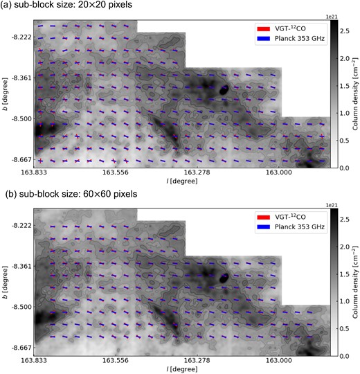
The magnetic field orientation inferred from the VGT using 12CO for sub-block sizes of 20 × 20 pixels (∼0.4 pc; top) and 60 × 60 pixels (∼1.2 pc; bottom) in the L1478 region of the CMC. VGT (red) and Planck polarization (blue) segments are overlaid in the integrated 12CO intensity map. Contours of both maps approximately at 1.3 × 10²¹, 1.4 × 10²¹, 1.6 × 10²¹, and 1.8 × 1021 cm−2.
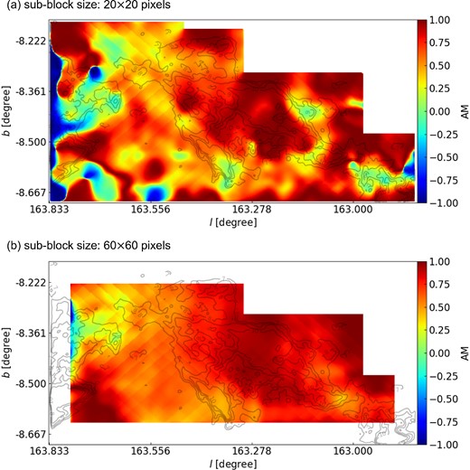
The distribution of AM calculated from the Planck and VGT measurements using 12CO for sub-block sizes of 20 × 20 pixels (∼0.4 pc; top) and 60 × 60 pixels (∼1.2 pc; bottom) in the L1478 region of the CMC. Red regions represent parallel alignment (i.e. AM values of positive one) and blue regions represent perpendicular alignment (i.e. AM values of negative one). Contours of both maps approximately at 1.3 × 10²¹, 1.4 × 10²¹, 1.6 × 10²¹, and 1.8 × 1021 cm−2.
The VGT-12CO-measured magnetic field map, as well as the corresponding AM distribution, at a resolution 3.3 arcmin (∼0.4 pc) are presented in Figs 1 and 2. The decrease in sub-block size reveals smaller scale variations of the magnetic field. In the 3.3 arcmin map, we see a much more perpendicular alignment of the VGT measurement with Planck polarization than in the 10 arcmin map, particularly for the eastern part. The disagreement here is purely caused by the difference in resolution. This suggests that the magnetic field at a smaller scale exhibits variation, which cannot be resolved by Planck polarization.
We further use 13CO and C18O emission lines to map the magnetic field. 13CO typically traces gas at a volume density ∼103 cm−3 and optically thin (optical depth ≪1) C18O traces denser gas at a density ∼104 cm−3. The application of VGT to the two tracers provides magnetic field information in denser regions. The VGT-13CO (or VGT-C18O) and Planck polarization have less alignment than in the case of VGT-12CO. At a resolution 10 arcsec, the mean AM of VGT-13CO and VGT-C18O is 0.42 and 0.49, respectively (see Table 1). The magnetic field and AM maps at resolution 10 arcmin are presented in Figs 3 and 4. Compared with VGT-12CO at 10 arcmin measurement (see Fig. 2), we see the appearance of more misalignment in 13CO and more perpendicular alignment in C18O. For 13CO, misalignment appears mostly in low-intensity regions, especially in the western and eastern part. In Fig. 6 at 10 arcmin, we see much of the regions with misalignment occurring around the AM value of −0.25. From Table 1), the mean AM value for 13CO at 10 arcmin is 0.42, which points to more misalignment than 12CO. One possibility for the misalignment is the contribution from the foreground and background dust polarization. It is known (see Liu et al. 2022), low-intensity regions typically correspond to low extinction. It is possible that in these low-extinction regions, the atomic H I or molecular 12CO foreground/background contribute more to the dust polarization. For C18O focusing only on a smaller central region, the majority of regions have a parallel alignment. We can see in Fig. 7 at 10 arcmin that the histogram spreads and is centred around more positive AM values than negative AM values, with a mean AM value of 0.49. In view that 12CO, 13CO, and C18 trace up to the volume density of 104 cm−3, the positive AM at resolution 10 arcmin suggests that L1478 globally is dominated by MHD turbulence and the self-gravity’s effect is not dominant up to volume density 104 cm−3.
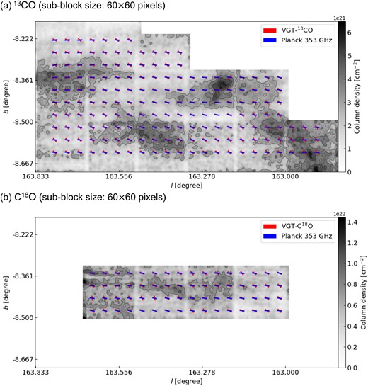
The magnetic field orientation inferred from the VGT using 13CO (top) and C18O (bottom) with sub-block sizes of 60 × 60 pixels (∼0.4 pc) in the L1478 region of the CMC. VGT gradient lines are represented in red and Planck polarization lines are represented in blue. Contours for top map are at 2.1 × 10²¹, 2.8 × 10²¹, 3.5 × 10²¹, and 4.1 × 1021 cm−2 and for bottom map are 6.6 × 10²¹, 8.8 × 10²¹, 1.1 × 10²², and 1.3 × 1022 cm−2.
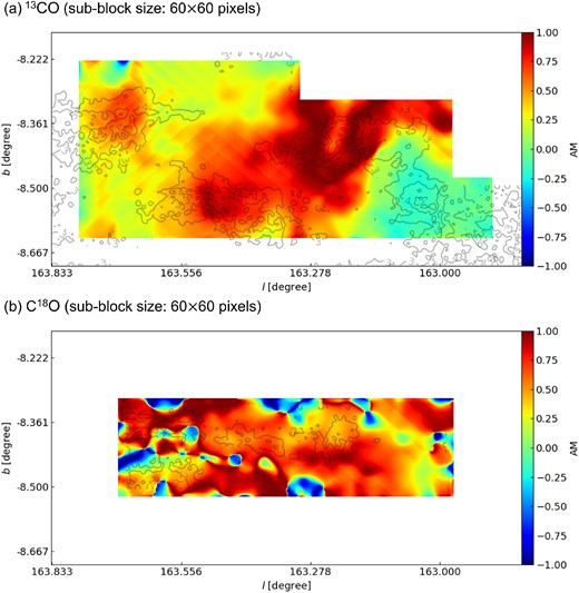
The AM distribution calculated from the Planck and VGT gradients using 13CO (top) and C18O (bottom) with sub-block sizes of 60 × 60 pixels (∼0.4 pc) in the L1478 region of the CMC. Contours for top map are at 2.1 × 10²¹, 2.8 × 10²¹, 3.5 × 10²¹, and 4.1 × 1021 cm−2 and for bottom map are 6.6 × 10²¹, 8.8 × 10²¹, 1.1 × 10²², and 1.3 × 1022 cm−2.
The histogram of AM values inferred from alignment between Planck Polarization and VGT using 12CO in the L1478 region of the CMC.
Same as Fig. 5, but for 13CO.
Same as Fig. 5, but for C18O.
While we identify magnetic fields using polarization, one must understand the limitations of this approach. Radiative torques (RATs) align grains in settings, where the radiation at the wavelength comparable to the dust size is sufficient (Lazarian & Hoang 2007). This, by itself, makes integration of the magnetic field along the line of sight inhomogeneous and different from the way that VGT probes magnetic fields. In addition, RATs can destroy grains (Hoang 2019). The dust grains aligned at attractor points with high angular momentum (Lazarian & Hoang 2021). The rotationally destroyed dust grains become too small to be spanned up and aligned by RATs. As a result, the sampling of the magnetic field by polarization can be inhomogeneous not only in denser, darker regions where RATs are weak but also in regions of high illumination where RATs are too strong.
4.2 L1482
L1482 is another subcloud of the CMC. It is located to the east of L1478, however, it shows higher column density (Lada et al. 2017; Zhang et al. 2018). The high column density suggests stronger self-gravity in L1482. As we discussed in Section 3, strong self-gravity could change the velocity gradient’s direction from perpendicular to parallel to the magnetic field. In terms of AM, such a change results in negative values. To exclude the difference in resolution size’s effect on VGT, we chose to mainly use the 60 × 60 sub-block sized (i.e. 10 arcmin) maps instead of 3.3 arcmin maps in order to examine the self-gravity’s effect on VGT and exclude the contribution from resolution differences.
The comparison of VGT and Planck, as well as the spatial distribution of AM, is presented in Figs 8 and 9. Considering the optically thick tracer 12CO, L1482 appears to have a mix of perpendicular alignment and parallel alignment spread out in clumps. Particularly, small northern region shows great alignment with AM larger than 0.60. The southern majority of the clump, however, exhibits more negative AM. The mean AM values for 3.3 and 10 arcmin are 0.06 and 0.02, respectively (see Table 1). These values are much lower than the mean AM values of L1478 when using 12CO as a tracer. Looking at denser tracer 13CO, much more negative-AM regions appear in Fig. 9 suggesting perpendicular alignment of velocity gradient and polarization. For 13CO, the mean AM values with 3.3 and 10 arcmin resolution are −0.22 and −0.40, respectively. These values are much more negative than our mean AM values for 12CO. This means there is much more perpendicular alignment at 13CO. The most apparent change is observed in small northern region. The positive AM >0.6 for VGT-12CO turns negative. Such change means that self-gravity starts dominating at volume density >103 cm−3, which is the density range traced by 13CO. Importantly, we find the negative AM typically appears in the ambient low-intensity region, while the high-density clump exhibits positive AM close to 1, which is even higher than that of VGT-12CO. This central clump corresponds to the location of the massive stellar cluster NGC1579 (Li et al. 2014), associated with a H ii expanding bubble and stellar wind (Herbig, Andrews & Dahm 2004). The H ii region may have more significant effects on changing diffuse molecular tracer 12CO’s dynamics so that VGT-12CO shows smaller AM than VGT-13CO.
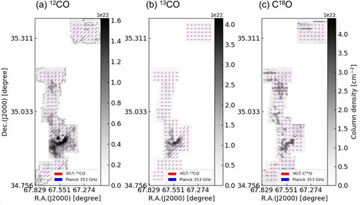
Magnetic field orientation inferred from the VGT using 12CO (left) with contours at 1.8 × 10²¹, 5.4 × 10²¹, 1.1 × 10²², and 1.4 × 1022 cm−2, 13CO (middle) with contours at 1.0 × 10²², 2.1 × 10²², 3.1 × 10²², and 3.8 × 1022 cm−2, and C18O (right) with contours at 1.3 × 10²², 2.2 × 10²², 3.1 × 10²², and 4.0 × 1022 cm−2, respectively for sub-block sizes of 60 × 60 pixels (∼1.2 pc) in the L1482 region of the CMC. VGT gradient lines are represented in red and Planck polarization lines are represented in blue.
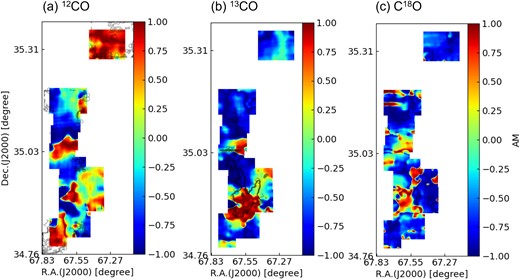
The AM inferred from the measurement of alignment of the Planck and VGT gradients using 12CO (left), 13CO (middle), and C18O (right), respectively, for sub-block sizes of 60 × 60 pixels (∼1.2 pc) in the L1482 region of the CMC. Red regions represent parallel alignment and AM values of one and blue regions represent perpendicular alignment with AM value of negative one.
This negative AM, however, is less likely to be contributed by the foreground or background magnetic fields because we do not expect a perpendicular alignment between the velocity gradient and the foreground or background magnetic fields. The possible explanation is that L1482 is under global gravitational contraction so that it is acreting ambient gas into the central dense clump. A stronger magnetic field and turbulence may counteract the collapse at the clump. This interesting phenomenon requires further studies.
As for the densest tracer C18O used in this work, we don’t see as much of a drastic change in perpendicular alignment, as we did when comparing 13CO to 12CO but there is still a minor magnitude increase in negative values. The mean AM values measured for C18O with 3.3 and 10 arcmin resolution2 are −0.29 and −0.45. This confirms our explanation that L1482 could be experiencing gravitational contraction at volume density >103 cm−3 so that we observed similar AM distribution for the denser tracers C18O.
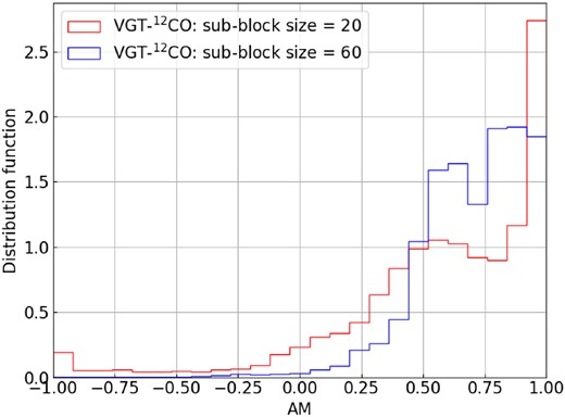
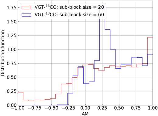
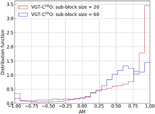
Furthermore, Figs 10, 11, and 12 present the histograms of the AM at two resolutions 10 and 3.3 arcmin. For VGT-12CO’s histogram, we see two peaks appears in AM = 1 and −1 suggesting the self-gravity’s effect occurs. As for VGT-13CO and VGT-C18O, the most apparent peak appears only on negative AM = −1. Particularly, the histogram at high resolution 3.3 arcmin is less dispersed than the 10 arcmin one due to the difference in VGT and Planck’s resolution. Nevertheless, the globally negative AM means self-gravity’s effect is significant in L1482.
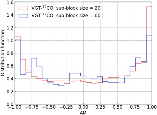
Same as Fig. 5, but for the L1482 region of the CMC.

Same as Fig. 10, but for 13CO.
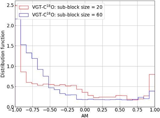
Same as Fig. 10, but for C18O.
5 DISCUSSION
5.1 The physical properties of L1478 and L1482
L1478 and L1482 are two subcloud of the giant CMC. Even though the two are closely located, they show very different physical properties. In our comparison of VGT and Planck polarization, we find in L1478 the velocity gradients are parallel to the magnetic field inferred from polarization, while in L1482 their relative orientation is mostly perpendicular.
According to earlier studies (Hu et al. 2020b), the parallel alignment suggests that self-gravity dominates over turbulence. It means L1482 at scales of order ∼1 pc undergoes global gravitational contraction. The ambient gas is accreting into the clump’s centre so that the velocity gradient is dominated by the contribution from the inflow. This agrees with the earlier study by Li et al. (2014) suggesting that L1482 is in the process of gravitational fragmentation and exhibits converging inflows. With VGT, we get more fruitful information. Such perpendicular alignment in L1482 is partially observed in VGT-12CO and is more apparent in VGT-13CO and VGT-C18O. Considering that 12CO, 13CO, and C18O typically trace molecular gas at volume density ranges ∼102, 103, and 104 cm−3, the significance of VGT-13CO and VGT-C18O reveals that the gravitational contraction mainly happens at volume density >103 cm−3.
The situation in L1478 gets different. The parallel alignment between the velocity gradients and the magnetic field inferred from polarization means turbulence is dominant and self-gravity’s effect is negligible. Particularly, we test the VGT at two resolutions 3.3 and 10 arcmin. We see that the alignment increases when comparing VGT and Planck at the same resolution of 10 arcmin. The difference observed in VGT and polarization measurements can be contributed by the difference in resolution. This important fact highlights the VGT’s advantage in tracing the magnetic field at smaller scales using emission lines.
5.2 Uncertainties
In this study, we investigate the L1478 and L1482 clouds by comparing VGT and Planck polarizations. We acknowledge several potential uncertainties in the comparison. Firstly, both VGT and Planck have inherent uncertainties. The uncertainty in VGT mainly stems from the sub-block averaging method and the noise in spectroscopic observations. To address these factors, we calculated the uncertainty maps of VGT, as demonstrated in Figs A1 and A2. Secondly, dust polarization and VGT rely on distinct physical mechanisms to trace magnetic fields, which may lead to misaligned magnetic field measurements between Planck and VGT. For example, dust polarization includes foreground/background emissions, whereas VGT directly probes the magnetic field associated with molecular clouds. Additionally, VGT uses molecular tracers 12CO, 13CO, and C18O, which are sensitive to different critical density values. The polarization based on RATs-aligned dust provides LOS integrated measurements, and the magnetic fields measured may be inhomogeneous if RATs are too strong in high-density regions. Despite these uncertainties, the overall statistically significant parallel (in L1478) and perpendicular (in L1482) alignments of VGT and Planck suggest that these factors are subdominated.
6 CONCLUSION
In this work, we use the velocity gradient technique (VGT) to trace the POS magnetic field orientation in the CMC’s two subclouds L1478 and L1482, and determine the dominance of MHD turbulence or self-gravity. We apply VGT to three emission lines 12CO, 13CO, and C18O to get information over the volume density range in approximately from 102 to 104 cm−3. We compare VGT results calculated in the resolutions of 3.3 and 10 arcmin to Planck polarization at 353 GHz and 10 arcmin to determine areas of MHD turbulence dominance and gravitational collapse dominance. Our main findings are:
We found the VGT-measured magnetic fields globally agree with that from Planck in L1478 suggesting self-gravity’s effect is insignificant. The best agreement appears in VGT-12CO.
For the turbulence-dominated cloud L1478, we use VGT with 12CO, 13CO, and C18O to provide magnetic field orientation maps at resolution ∼3.3 arcmin, higher than Planck polarization.
We show that the resolution difference can introduce misalignment between VGT and Planck polarization measurement.
As for L1482, the VGT measurements are statistically perpendicular to the Planck polarization indicating the dominance of self-gravity. This perpendicular alignment is more significant in VGT-13CO and VGT-C18O.
ACKNOWLEDGEMENTS
Y.H. and A.L. acknowledges the support of NASA ATP AAH7546. Financial support for this work was provided by NASA through award 09_0231 issued by the Universities Space Research Association, Inc. (USRA).
DATA AVAILABILITY
The data underlying this article will be shared on reasonable request to the corresponding author.
Footnotes
We present only the gradient vector maps at 10 arcmin to avoid the confusion of resolution difference and self-gravity effect. However, we conducted the calculation for both 3.3 and 10 arcmin and we list the AM value in table.
References
APPENDIX A: UNCERTAINTY MAPS
Figs A1 and A2 present the uncertainty maps of our VGT measurements. Such uncertainties can be mostly attributed to the systematic error in the observational data as well as the VGT algorithm. As introduced in Section 3, the algorithm fits the gradient’s orientations over predetermined subregions into a Gaussian histogram and yields the angle at which the peak value of the histogram exists. This error from the Gaussian fitting algorithm within the 95 per cent confidence level is denoted as |$\sigma _{\psi _{\rm gs}} (x, y, v)$|, and thus the uncertainties are obtained as such:
where |$\sigma _{\psi_{\rm g}}$| is the angular uncertainty of the magnetic field measurements, σn(x, y, v) denotes the noise in velocity channel Ch(x, y, v) as well as error propagation, and σQ(x, y), σU(x, y) give the respective uncertainty of the pseudo-Stokes parameters Qg(x, y), Ug(x, y).
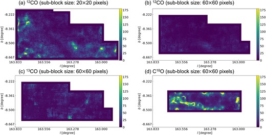
Uncertainty maps for L1478. The color bar is in the unit of degrees with range 0°–180°.
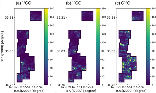
Uncertainty maps for L1482. The color bar is in the unit of degrees with range 0°–180°.
APPENDIX B: LINE SPECTRA
Fig. B1 presents the averaged line spectra for L1478 and L1482. In L1478, the 12CO line exhibits a maximum intensity of approximately 1.7 K, while the 13CO line shows a lower intensity, with a maximum of around 0.55 K. The C18O line has an even lower intensity with a maximum of about 0.04 K. All three spectra have different noise levels, with 12CO having a higher noise level of below 0.05 K compared to 13CO and C18O, which have noise levels below 0.02 and 0.005 K, respectively. In addition, for L1482, the 12CO line exhibits a higher maximum intensity of approximately 1.4 K, while the 13CO and C18O lines have lower intensities with maximum values of around 0.65 and 0.09 K, respectively. The noise levels for the three lines also differ, with 12CO having a higher noise level of below 0.1 K, 13CO having a noise level below 0.03 K, and C18O having a noise level below 0.005 K. Both L1487 and L1482 are dominated by a single velocity component.
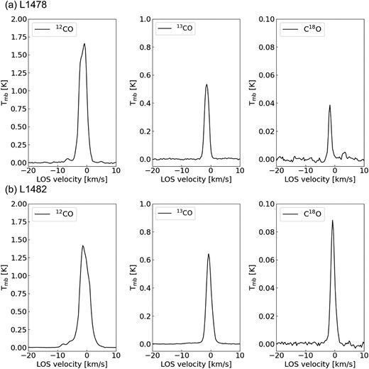
Average line spectra for L1478 and L1482.
APPENDIX C: SUB-BLOCK AVERAGING
The sub-block averaging method implemented in VGT requires that the sampled gradients form a Gaussian distribution. Here, we present a test for this requirement. In Fig. C1, we plot the histogram of gradient orientation for two randomly selected sub-blocks within L1478. The two sub-blocks have sizes of 20 × 20 and 60 × 60 pixels, respectively. The histogram exhibits two apparent Gaussian distributions.
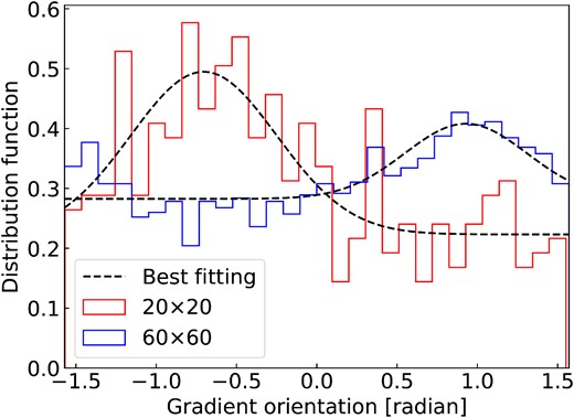
Histogram of gradient orientation for two randomly selected sub-blocks within L1478.
