


ABSTRACT
A variety of observational campaigns seek to test dark matter models by measuring dark matter subhaloes at low masses. Despite their predicted lack of stars, these subhaloes may be detectable through gravitational lensing or via their gravitational perturbations on stellar streams. To set measurable expectations for subhalo populations within Lambda cold dark matter, we examine 11 Milky Way (MW)-mass haloes from the FIRE-2 baryonic simulations, quantifying the counts and orbital fluxes for subhaloes with properties relevant to stellar stream interactions: masses down to |$10^{6}\, \text{M}_\odot$|, distances ≲50 kpc of the galactic centre, across z = 0 − 1 (tlookback = 0–8 Gyr). We provide fits to our results and their dependence on subhalo mass, distance, and lookback time, for use in (semi)analytical models. A typical MW-mass halo contains ≈16 subhaloes |$\gt 10^{7}\, \text{M}_\odot$| (≈1 subhalo |$\gt 10^{8}\, \text{M}_\odot$|) within 50 kpc at z ≈ 0. We compare our results with dark matter-only versions of the same simulations: because they lack a central galaxy potential, they overpredict subhalo counts by 2–10×, more so at smaller distances. Subhalo counts around a given MW-mass galaxy declined over time, being ≈10× higher at z = 1 than at z ≈ 0. Subhaloes have nearly isotropic orbital velocity distributions at z ≈ 0. Across our simulations, we also identified 4 analogues of Large Magellanic Cloud satellite passages; these analogues enhance subhalo counts by 1.4–2.1 times, significantly increasing the expected subhalo population around the MW today. Our results imply an interaction rate of ∼5 per Gyr for a stream like GD-1, sufficient to make subhalo–stream interactions a promising method of measuring dark subhaloes.
1 INTRODUCTION
A key prediction of the cold dark matter (CDM) model is the existence of effectively arbitrarily low-mass self-gravitating dark matter (DM) structures, known as haloes, including subhaloes that reside within a more massive halo (Klypin et al. 1999; Moore et al. 1999; Springel et al. 2008; Bullock & Boylan-Kolchin 2017). Alternative models, such as warm dark matter (WDM) and fuzzy DM, predict a lower cutoff in the (sub)halo mass function (e.g. Hu, Barkana & Gruzinov 2000; Ostdiek, Diaz Rivero & Dvorkin 2022). Current constraints on low-mass (sub)haloes come from luminous galaxies, such as the faint satellite galaxies around the Milky Way (MW). Measurements of ultrafaint galaxies imply that (sub)haloes exist down to |$\sim 10^{8} \, \text{M}_\odot$| (e.g. Jethwa, Erkal & Belokurov 2018; Nadler et al. 2021). Theoretical works show that (sub)haloes below this mass are below the atomic cooling limit and therefore unable to retain enough gas before cosmic reionization to support star formation, leaving them starless and thus invisible to direct detection (e.g. Bullock, Kravtsov & Weinberg 2000; Benson et al. 2002; Somerville 2002). The discovery of completely dark (sub)haloes would represent another key success of the CDM model, and such measurement (or lack thereof) would provide key constraints on the properties of DM.
To date, researchers have devised two potential avenues for indirectly detecting these dark (sub)haloes. One method uses gravitational lensing: the lensed light from a background galaxy allows us to determine a foreground galaxy’s mass distribution (Mao & Schneider 1998), including low-mass (sub)haloes that reside along the line of sight. Most work using this method focuses on population statistics (Ostdiek et al. 2022; Şengül & Dvorkin 2022; Wagner-Carena et al. 2023), although Vegetti et al. (2012, 2014) identified individual satellites with total mass |$10^{8}\!-\!10^{9} \, \text{M}_\odot$| at z ≈ 0.2–0.5. Existing works predominantly examine galaxies with DM halo masses |$M_{\rm halo} \gtrsim 10^{13} \, \text{M}_\odot$| at these redshifts, notably higher than MW-mass galaxies with |$M_{\rm halo} \approx 10^{12} \, \text{M}_\odot$| at z = 0 (e.g. Bland-Hawthorn & Gerhard 2016).
The MW itself provides a separate means to measure dark subhaloes, via perturbations to thin streams of stars that originate from the tidal disruption of a globular cluster (GC) or satellite galaxy?? (Ibata et al. 2002; Johnston 2016). If a subhalo passes near such a stellar stream, its gravitational field can impart an identifiable gap, spur, or other perturbation, whose properties depend on the subhalo’s mass, size, velocity, and other orbital parameters. Recent works explored how subhaloes with masses |$\gtrsim 10^{5} \, \text{M}_\odot$| can induce observable features in stellar streams?? (e.g. Yoon, Johnston & Hogg 2011; Erkal et al. 2016; Banik et al. 2018; Bonaca et al. 2019); less massive subhaloes lack the energy necessary to leave observable evidence of interaction. To confirm that a dark subhalo induced a particular perturbation, one must rule out the effects of luminous objects, including the MW’s > 50 known satellite galaxies (McConnachie 2012; Simon 2019) and >150 known GCs (Harris 2010), as well as giant molecular clouds (Amorisco et al. 2016) and other stellar streams (Dillamore et al. 2022).
Of the dozens of currently well-known streams around the MW (e.g. Grillmair & Carlin 2016; Mateu 2023), most studies focus on two, GD-1 and Pal 5, given their relative proximity to the MW and the high-quality 6D phase-space data available for them. GD-1 is ≈15 kpc long, with a pericentre of 13 kpc and apocentre of 27 kpc, and it formed ≈3 Gyr ago (Doke & Hattori 2022), likely from a progenitor GC (Bonaca & Hogg 2018). Pal 5 is ≈10 kpc long (Starkman, Bovy & Webb 2020), with a pericentre of 8 kpc and an apocentre of 19 kpc (Yoon et al. 2011), and it formed ≈8 Gyr ago from the Pal 5 GC (Odenkirchen et al. 2001). GD-1 and Pal 5 represent perhaps the ideal streams on which to study the potential gravitational impacts of dark subhaloes, though Gaia data release 3 (DR3) now provides even more detailed 6D phase-space measurements of stars in more streams (Gaia Collaboration 2021).
In addition to the subhaloes orbiting the MW itself, the CDM model also predicts that large satellites such as the Large Magellanic Cloud (LMC) host their own orbiting subhaloes (e.g. Deason et al. 2015; Sales et al. 2016; Jahn et al. 2019; Santos-Santos et al. 2021). Given that the LMC just passed its pericentre of d ≈ 50 kpc from the MW centre (Kallivayalil et al. 2013), the inner halo currently may be in a temporary period of enhanced subhalo enrichment (Dooley et al. 2017a, b).
Theoretical predictions for the counts, orbits, and sizes of dark subhaloes can help support or rule out a dark subhalo origin for observed gaps or other features in stellar streams. Previous works have predicted subhalo populations in the mass regime relevant to subhalo–stream interactions (|$\approx 10^{5}\!-\!10^{8} \, \text{M}_\odot$|). Most used dark matter-only (DMO) simulations that do not account for the effects of baryonic matter (e.g. Yoon et al. 2011; Mao, Williamson & Wechsler 2015; Griffen et al. 2016). However, incorporating baryonic physics significantly can affect subhalo populations. Primarily, the presence of the central galaxy induces additional tidal stripping on subhaloes that orbit near it, which, as previous works (e.g. D’Onghia et al. 2010; Garrison-Kimmel et al. 2017; Webb & Bovy 2020) showed, causes DMO simulations to overpredict subhalo count significantly, by 5× or more, near the central galaxy. Additionally, gas heating from the cosmic UV background reduces the initial masses and subsequent accretion history of low-mass (sub)haloes, making them lower mass today (e.g. Bullock et al. 2000; Benson et al. 2002; Somerville 2002).
The FIRE-2 cosmological zoom-in simulations are well suited for predicting the population of low-mass dark subhaloes, given their high resolution and inclusion of relevant baryonic physics; most importantly, the formation of realistic MW-mass galaxies. As a critical benchmark, previous works have shown that the luminous subhaloes (satellite galaxies) around MW-mass galaxies in FIRE-2 broadly match the distributions of stellar masses and internal velocities (Wetzel et al. 2016; Garrison-Kimmel et al. 2019), as well as radial distance distributions (Samuel et al. 2020), of satellite galaxies observed around the MW and M31, as well as MW analogues in the SAGA survey (Geha et al. 2017). Furthermore, as Samuel et al. (2021) showed, FIRE-2 MW-mass galaxies with an LMC-like satellite show much better agreement with various metrics of satellite planarity, as observed around the MW and M31, which motivates further exploration of potential effects of the LMC on the population of low-mass, dark subhaloes.
In this work, we extend these FIRE-2 predictions of satellite populations down to lower mass subhaloes, with DM masses as low as |$10^{6} \, \text{M}_\odot$|, which, as we described above, are likely to be completely dark (devoid of stars). We examine subhaloes within 50 kpc of MW-mass galaxies, the regime most relevant for observable interactions of dark subhaloes with stellar streams. We expand in particular on the work of Garrison-Kimmel et al. (2017); we examine subhaloes across a much larger set of 11 MW-mass haloes (instead of 2), and we time-average over multiple simulation snapshots (instead of just the one at z = 0) for improved statistics for the small number of subhaloes that survive near the MW-mass galaxy.
2 METHODS
2.1 FIRE-2 simulations of MW-mass haloes
We analyse simulated host galaxy haloes from the FIRE-2 cosmological zoom-in simulations (Hopkins et al. 2018). We generated each simulation using gizmo (Hopkins 2015), which models N-body gravitational dynamics with an updated version of the gadget-3 TreePM solver (Springel 2005), and hydrodynamics via the meshless finite-mass method. FIRE-2 incorporates a variety of gas heating and cooling processes, including free–free radiation, photoionization and recombination, Compton, photoelectric and dust collisional, cosmic ray, molecular, metal-line, and fine-structure processes, including 11 elements (H, He, C, N, O, Ne, Mg, Si, S, Ca, and Fe). We use the model from Faucher-Giguère et al. (2009) for the cosmic UV background, in which H i reionization occurs at z ≈ 10. Each simulation consists of DM, star, and gas particles. Star formation occurs in gas that is self-gravitating, Jeans-unstable, cold (T < 104 K), dense (n > 1000 cm−3), and molecular as in Krumholz & Gnedin (2011). Once formed, star particles undergo several feedback processes, including core-collapse and Type Ia supernovae, continuous stellar mass-loss, photoionization and photoelectric heating, and radiation pressure.
We generated cosmological initial conditions for each simulation at z ≈ 99, within periodic boxes of length 70.4–172 Mpc using the MUSIC code (Hahn & Abel 2011). We assume flat ΛCDM cosmologies, with slightly different parameters across our host selection: h = 0.68 − 0.71, ΩΛ = 0.69 − 0.734, Ωm = 0.266 − 0.31, Ωb = 0.0455 − 0.048, σ8 = 0.801 − 0.82, and ns = 0.961 − 0.97, broadly consistent with Planck Collaboration VI (2020). We saved 600 snapshots from z = 99 to 0, with typical spacing ≲25 Myr.
We examine host haloes from two suites of simulations. The first is the Latte suite of individual MW-mass haloes (introduced in Wetzel et al. 2016), which have DM halo masses of |$M_{200\textrm {m}} = 1 \!-\! 2 \times 10^{12} \, \text{M}_\odot$| and no neighboring haloes of similar or greater mass within at least ≈5R200m, where R200m is defined as the radius within which the density is 200 times the mean matter density of the Universe. Gas cells and star particles have initial masses of |$7070 \, \text{M}_\odot$|, while DM particles have a mass of |$3.5 \times 10^{4} \, \text{M}_\odot$|. Latte uses gravitational force softening lengths of 40 pc for DM and 4 pc for star particles (comoving at z > 9 and physical thereafter), and the gravitational softening for gas is adaptive, matching the hydrodynamic smoothing, down to 1 pc. We also examine host haloes from the ELVIS on FIRE suite of Local Group-like MW + M31 halo pairs (introduced in Garrison-Kimmel et al. 2019). These simulations have ≈2× better mass resolution than Latte: Romeo & Juliet have initial masses of |$3500 \, \text{M}_\odot$| for baryons and |$1.9 \times 10^{4} \, \text{M}_\odot$| for DM, while Romulus & Remus and Thelma & Louise have initial masses of |$4000 \, \text{M}_\odot$| for baryons and |$2.0 \times 10^{4} \, \text{M}_\odot$| for DM. ELVIS uses gravitational force softening lengths of ≈32 pc for DM, 2.7–4.4 pc for stars, and 0.4–0.7 pc (minimum) for gas.
To ensure similarity to the MW, we selected host galaxies from these suites that have a stellar mass within a factor of ≈2 of |$M_{\textrm {MW}} \approx 5 \times 10^{10} \, \text{M}_\odot$| (Bland-Hawthorn & Gerhard 2016), which leaves 11 total hosts: 6 from Latte and 5 from ELVIS. Table 1 lists their properties at z ≈ 0. For each simulation, we also generated a DMO version at the same resolution, and we compare these against our baryonic simulations to understand the effects of baryons on subhalo populations. The primary effect of baryons for our analysis of low-mass subhaloes is simply the additional gravitational potential of the MW-mass galaxy (Garrison-Kimmel et al. 2017).
Properties of the MW/M31-mass galaxies/haloes at z ≈ 0 in the FIRE-2 simulations. We include galaxies with |$M_\text{star}= 2.5 \!-\! 10 \times 10^{10} \, \text{M}_\odot$|, within a factor of ≈2 of the MW. The last 3 columns list the number of subhaloes above the given threshold in instantaneous DM mass that are within 50 kpc of the host, time-averaged across z = 0 − 0.15 (1.9 Gyr).
| Name | Mstar | |$M_{200\rm {m}}$| | Mtotal(< 100 kpc) | Nsubhalo | Nsubhalo | Nsubhalo | Introduced in |
|---|---|---|---|---|---|---|---|
| (|$10^{10} \, \text{M}_\odot$|) | (|$10^{12} \, \text{M}_\odot$|) | (|$10^{11} \, \text{M}_\odot$|) | |$(\gt 10^6 \, \text{M}_\odot)$| | |$(\gt 10^7 \, \text{M}_\odot)$| | |$(\gt 10^8 \, \text{M}_\odot)$| | ||
| m12m | 10.0 | 1.6 | 7.9 | 123 | 21.3 | 1.4 | [1] |
| Romulus | 8.0 | 2.1 | 10.4 | 143 | 16.4 | 1.8 | [2] |
| m12b | 7.3 | 1.4 | 7.2 | 90 | 14.0 | 0.9 | [2] |
| m12f | 6.9 | 1.7 | 8.0 | 106 | 18.2 | 1.4 | [3] |
| Thelma | 6.3 | 1.4 | 7.7 | 179 | 30.9 | 2.7 | [2] |
| Romeo | 5.9 | 1.3 | 7.7 | 168 | 18.9 | 1.6 | [2] |
| m12i | 5.5 | 1.2 | 6.4 | 131 | 20.4 | 1.9 | [4] |
| m12c | 5.1 | 1.4 | 6.2 | 246 | 47.4 | 4.2 | [2] |
| m12w | 4.8 | 1.1 | 5.5 | 162 | 18.8 | 1.9 | [5] |
| Remus | 4.0 | 1.2 | 6.8 | 132 | 20.4 | 2.3 | [2] |
| Juliet | 3.4 | 1.1 | 5.9 | 207 | 29.2 | 2.5 | [2] |
| average | 6.1 | 1.4 | 5.9 | 153 | 23.3 | 2.1 |
2.2 Finding and measuring subhaloes
We examine subhaloes, which we define as lower-mass haloes that reside within a R200m of a MW-mass host halo. We identify DM subhaloes using the rockstar 6D halo finder (Behroozi, Wechsler & Wu 2012a), defining (sub)haloes as regions of space with a DM density >200× the mean matter density. We include subhaloes that have a bound mass fraction of >0.4 and at least 30 DM particles, then construct merger trees using CONSISTENT-TREES (Behroozi et al. 2012b). For numerical stability, we first generate (sub)halo catalogues using only DM particles, then we assign star particles to haloes in post-processing (see Samuel et al. 2020).
From the merger trees, we select subhaloes with masses, distances, and redshifts that are most relevant for observable gravitational interactions with stellar streams (as in Koposov, Rix & Hogg 2010; Thomas et al. 2016; Li et al. 2022). Throughout, we examine subhaloes according to their instantaneous mass, given that this mass, rather than the pre-infall ‘peak’ mass, is more relevant for the strength of stream interactions (or the strength of gravitational lensing perturbations). We examine three thresholds in instantaneous mass: Msub > 106, >107, and |$\gt 10^{8} \, \text{M}_\odot$|, corresponding to a minimum of ≈30–60, 300–600, and 3000–6000 DM particles, being lower in the Latte simulations and higher in the ELVIS Local Group-like simulations. These subhaloes typically had ≳4× higher mass (more DM particles) prior to MW infall and tidal mass stripping, independent of subhalo mass. When examining subhaloes in DMO simulations, we reduce their masses by the cosmic baryon mass fraction (≈15 per cent), assuming that these subhaloes would have lost essentially all of their baryonic mass, consistent with the properties of subhaloes at these masses in our baryonic simulations (see also Bullock & Boylan-Kolchin 2017).
We include all subhaloes above these mass thresholds regardless of whether they are luminous or dark. For subhaloes within 50 kpc, the fraction that contain at least 6 star particles (the limit of our galaxy catalog) is: 30 per cent at |$M_{\rm sub} \gt 10^{8} \, \text{M}_\odot$|, 5 per cent at |$M_{\rm sub} \gt 10^{7} \, \text{M}_\odot$|, and ≲ 1 per cent at |$M_{\rm sub} \gt 10^{6} \, \text{M}_\odot$|.
In Appendix A, we explore the resolution convergence of our results. In summary, our tests show that the counts of subhaloes with |$M_{\rm sub} \gt 10^{7} \, \text{M}_\odot$| are well converged, but our simulations likely underestimate subhalo counts at |$M_{\rm sub} \gt 10^{6} \, \text{M}_\odot$| by up to ≈1.5 − 2 (depending on distance) at z ≈ 0, so one should consider those results as lower limits to the true counts. We show results for |$M_{\textrm {sub}} \gt 10^{6} \, \text{M}_\odot$| in a lighter shade to reinforce this caution.
We use three metrics to quantify subhalo counts: number enclosed, number density, and orbital radial flux. The number enclosed, N(< d), includes all subhaloes within a given distance d from the host galaxy centre. We calculate the subhalo number density, n(d), by counting all subhaloes within a spherical shell 5 kpc thick, with the shell midpoint centred at d, and dividing by the volume of the shell. To inform predictions for subhalo–stream interaction rates, we also include the subhalo orbital radial flux, f(d), or the amount of subhaloes passing into or out of a host-centred spherical surface of radius d per Gyr. We count a subhalo as passing through the surface if, between two adjacent snapshots, it orbited from outside to inside the surface or vice versa. We do not distinguish between inward and outward flux. While our snapshot spacing of 20–25 Myr provides good time resolution, we also interpolate the distances of subhaloes between snapshots. For each subhalo within 5 kpc of a given distance bin, we apply a cubic spline fit to its distance from the host for several snapshots surrounding the current snapshot to determine its distance between snapshots. Using these interpolated distances is important at small d, where the surface-crossing times are shortest: it increases the measured flux by ≈20 per cent at d < 10 kpc compared to using the snapshots alone. We will also show that, at z ≈ 0, subhaloes have approximately isotropic orbits on average, so our values for radial flux can be used as flux rates in any direction at low redshifts.
We examine trends back to z = 1 (lookback time tlb ≈ 8 Gyr), because observable dynamical perturbations to stellar streams could have occurred several Gyr ago (see Yoon et al. 2011). Furthermore, because subhalo counts are subject to time variability and Poisson noise, especially at small distances, given that an orbit spends the least time near pericentre, we follow the approach in Samuel et al. (2020): for each host halo, we time-average its subhalo population across 92 snapshots at z = 0 − 0.15 (tlb = 0 − 2.15 Gyr). We then compute the median and 68 per cent distribution across the 11 host haloes. When examining redshift evolution, we average over 3 redshift ranges: z = 0.0 − 0.1 (tlb = 0 − 1.3 Gyr, 66 snapshots), z = 0.5 − 0.6 (tlb = 5.1 − 5.7 Gyr, 25 snapshots), and z = 1.0 − 1.1 (tlb = 7.8 − 8.2 Gyr, 14 snapshots).
We use the publicly available python packages, gizmoanalysis (Wetzel & Garrison-Kimmel 2020a), and haloanalysis (Wetzel & Garrison-Kimmel 2020b) to analyse these data.
2.3 LMC satellite analogues
Numerous works have demonstrated the likely contribution of the LMC to the population of luminous satellite galaxies around the MW (e.g. Hargis, Willman & Peter 2014; Deason et al. 2015; Jethwa, Erkal & Belokurov 2016; Sales et al. 2016; Dooley et al. 2017a, b; Patel et al. 2020). This motivates the possibility that the LMC also may have contributed a significant fraction of non-luminous lower-mass subhaloes as well. To assess if the presence of the LMC today affects predictions for subhaloes close to the MW, we select host haloes that contain a satellite that is an analogue to the LMC, following Samuel et al. (2022), with the following constraints:
Pericentric passage at tlb < 6.4 Gyr (z < 0.7): we choose this broad time window to capture a larger number of (rare) LMC-like passages.
|$M_\mathrm{sub,peak} \gt 4 \times 10^{10} \, \text{M}_\odot$| or |$M_\text{star}\gt 5 \times 10^{8} \, \text{M}_\odot$|: consistent with observations and inferences of the LMC’s mass (see Erkal et al. 2019; Vasiliev, Belokurov & Erkal 2021).
dperi < 50 kpc: consistent with the current measured pericentric distance of the LMC (see Kallivayalil et al. 2013).
The satellite is at its first pericentric passage, consistent with several lines of evidence that suggest that the LMC is on its first infall into the MW (see Kallivayalil et al. 2013; Sales et al. 2016).
From our 11 MW-mass haloes, this leaves 4 LMC analogues that meet all 4 criteria. Table 2 lists their properties, including masses and pericenters. Because we are interested in how the LMC affects recent MW subhalo populations, we show properties of each LMC satellite analogue when it first reached a distance of 50 kpc from the galaxy centre, corresponding to the LMC’s current distance.
Properties of the 4 LMC satellite analogues, at the lookback time that each one first orbits within a distance of 50 kpc from their MW-mass host galaxy.See Section 2.3 for details on their selection criteria. While we list the actual (initial) pericentric distance of their orbit, we present all results when these satellites first were at d ≈ 50 kpc, to provide context for the LMC at its current distance.Msub,inst indicates the instantaneous subhalo DM mass of the LMC analog this time, while Msub,peak is its peak (sub)halo mass throughout its history.
| Host | |$t^{\textrm {lb}}_{\rm 50 \ kpc}$| (Gyr) | z50 kpc | Mstar (|$10^{9} \, \text{M}_\odot$|) | Msub,inst (|$10^{11} \, \text{M}_\odot$|) | Msub,peak (|$10^{11} \, \text{M}_\odot$|) | dperi (kpc) |
|---|---|---|---|---|---|---|
| m12w | 6.0 | 0.60 | 1.25 | 0.9 | 1.3 | 8 |
| m12b | 5.1 | 0.50 | 7.13 | 1.7 | 2.1 | 38 |
| m12f | 3.1 | 0.27 | 2.62 | 1.1 | 1.6 | 36 |
| m12c | 1.0 | 0.08 | 1.17 | 1.2 | 1.7 | 18 |
3 RESULTS
3.1 Counts and orbital radial fluxes
In Fig. 1, we characterize subhalo counts via three metrics: (1) the cumulative number of subhaloes, N(< d), within a spherical shell at distance d from the MW-mass galaxy centre; (2) the number density of subhaloes, n(d), within ±2.5 kpc of d, and (3) the orbital radial flux of subhaloes through a spherical surface at d, including both incoming and outgoing subhaloes. We show each metric for three thresholds in subhalo instantaneous DM mass: Msub > 106, 107, and |$10^{8} \, \text{M}_\odot$|. Here and throughout, we show results for |$M_\textrm {sub} \gt 10^{6} \, \text{M}_\odot$| with a lighter shade, to emphasize that those counts are likely lower limits, given the resolution considerations in Appendix A.
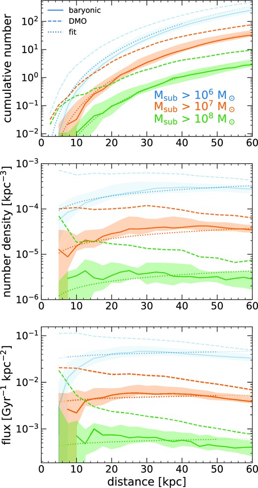
Counts and orbital radial fluxes of DM subhaloes as a function of distance, d, from the central MW-mass galaxy at z ≈ 0. For each halo, we time-average its subhalo population over 92 snapshots across z = 0 − 0.15 (1.9 Gyr). Solid lines and shaded regions show the median and 68 per cent distribution across the 11 host haloes. We show results for |$M_{\rm sub} \gt 10^{6} \, \text{M}_\odot$| in a lighter shade to indicate potential resolution effects (see Section 2.2). Dashed lines show DMO simulations of the same haloes. Dotted lines show the fits in Table 3; a lighter shade indicates points outside of the distance range used for fitting. Top: Cumulative number of subhaloes, N(< d), within sphere of radius d. Middle: Number density, n(d), of subhaloes within a spherical shell ±2.5 kpc of d. Bottom: Orbital radial flux of subhaloes, that is, the number of subhaloes per kpc2 per Gyr passing either inwards or outwards through a spherical surface of radius d. Because of the additional gravitational tidal stripping from the MW-mass galaxy in the baryonic simulations (unlike in the DMO simulations), both n(d) and flux vary only weakly with d, to within a factor of a few.
All three metrics of subhalo counts decrease roughly linearly with increasing subhalo mass at a given d. Within the approximate orbital distances of GD-1 and Pal 5, d ≈ 10–30 kpc (Price-Whelan & Bonaca 2018), we predict ≈4 subhaloes of |$M_\textrm {sub} \gt 10^{7} \, \text{M}_\odot$| and at least 20 subhaloes of |$M_\textrm {sub} \gt 10^{6} \, \text{M}_\odot$|. We find no significant differences in subhalo counts between Latte hosts and ELVIS hosts. Interestingly, both number density and flux vary only weakly with d, to within a factor of a few. This is in contrast with the DMO simulations, which show a strong rise in these quantities towards smaller d. Unlike Garrison-Kimmel et al. (2017), who analysed only the snapshot at z = 0, our averaging across multiple snapshots reveals significant populations of subhaloes at small d.
Fig. 2 quantifies the differences between the baryonic and DMO simulations, showing the ratio of the number density, n(d), at a given d, given that many previous works used DMO simulations to explore subhalo populations. Subhalo counts in baryonic simulations are systematically smaller than those in DMO, especially at small d, primarily because of the additional gravitational tidal stripping from the MW-mass galaxy (e.g. Garrison-Kimmel et al. 2017; Kelley et al. 2019). DMO simulations overpredict subhalo counts by ≈2–3× at d ≈ 50 kpc and by an order of magnitude at d ≲ 10 kpc, across all mass thresholds. At our fiducial stellar stream distances of d ≈ 10–30 kpc, the ratio is ≈0.05–0.25 (that is, 4–20× more subhaloes in DMO simulations). These results are similar to Samuel et al. (2020), who analysed more-massive, luminous subhaloes with |$M_\textrm {peak} \gt 8 \times 10^{8} \, \text{M}_\odot$| in the same simulations, and found good agreement in the radial distance distribution with observations of satellites around the MW and M31. Fig. 2 shows their fit for the ratio of luminous satellites to DMO subhaloes via the dotted line, being ≈0.3 at d ≈ 50 kpc.
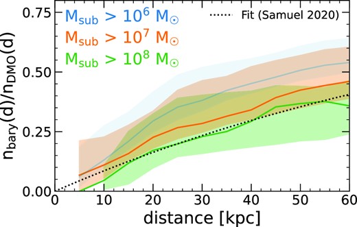
Ratio of the number density of subhaloes at z ≈ 0 (as in Fig. 1, middle) in baryonic simulations relative to DMO versions of the same host haloes. We show the median and 68 per cent distribution across the 11 haloes. This ratio illustrates the significant depletion of subhaloes in baryonic simulations, especially at small d, primarily from the increased gravitational tidal stripping from the presence of the MW-mass galaxy. The typical ratio at d = 10–30 kpc, the approximate distances of the GD-1 and Pal-5 streams, is 0.05–0.25, so DMO simulations overpredict subhalo counts by 4–20×. We show the fit from Samuel et al. (2020) for more massive (luminous) subhaloes, with |$M_\textrm {sub,peak} \gt 8 \times 10^{8} \, \text{M}_\odot$|, as a dotted line, which matches well our results at |$M_\textrm {sub} \gt 10^{8} \, \text{M}_\odot$|.
Fig. 3 shows the same metrics as Fig. 1, for only subhaloes with |$M_{\rm sub} \gt 10^{7} \, \text{M}_\odot$|, at 3 redshifts: z ≈ 0, ≈0.5, and ≈1 (still averaged across multiple snapshots, see Section 2.2). All subhalo counts decreased over cosmic time at a given d; from z = 1 to z = 0, subhalo number density declined by a factor of ≈15. We expect such a decline because, as explored in (for example Wetzel, Cohn & White 2009), subhalo merging and destruction rates at earlier times are faster than the infall rate of new subhaloes, given the decline in overall accretion rate as the Universe expands. This decline occurred in both baryonic and DMO simulations, but at small d, the decrease over time is more significant in the baryonic simulations, given the higher rates of tidal stripping from the MW-mass galaxy. We find decreases of ≈20 × at d = 10 kpc and ≈3 × at d = 50 kpc from z = 1 to z = 0.
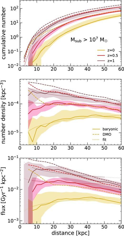
Counts and orbital radial flux versus distance, d, from the MW-mass galaxy, for DM subhaloes with |$M_{\rm sub} \gt 10^{7} \, \text{M}_\odot$| at different redshifts. We show the median and 68 per cent distribution across the 11 host haloes. We time-average each one over the range z = 0–0.1, 0.5–0.6, and 1–1.1, corresponding to lookback times 0–1.3, 5.1–5.7, and 7.8–8.2 Gyr. Dashed lines show median values for DMO simulations of the Latte hosts. Dotted lines show the fits from Table 3; a lighter shade indicates points outside of the distance range used for fitting. Top: Cumulative number, N(< d), within a sphere of radius d. Middle: Number density, n(d), within a spherical shell ±2.5 kpc of d. Bottom: Orbital radial flux, that is, the number of subhaloes per Gyr passing in and out of a spherical surface of radius d. All subhalo counts decrease over cosmic time, by up to ≈20× at d = 10 kpc, and less dramatically (∼3×) at d = 50 kpc. The counts of subhaloes in baryonic simulations decreased more dramatically than in DMO simulations (≈4× at most), especially at small d, because of additional tidal stripping from the MW-mass galaxy.
Fig. 4 quantifies this decrease over time, for the three mass thresholds, via the ratio of N(<50 kpc) at a given lookback time to the same value today. In baryonic simulations, this decrease has a slight mass dependence, while declines are similar across all masses in the DMO versions. Thus, using subhalo counts only at z = 0 would underestimate the subhalo population averaged across the last several Gyr, especially if the observable impacts on stellar streams persist for several Gyr. Our results at higher redshift also inform typical gravitational lensing studies, given that most observed lenses for measuring (sub)halo populations are at z > 0.
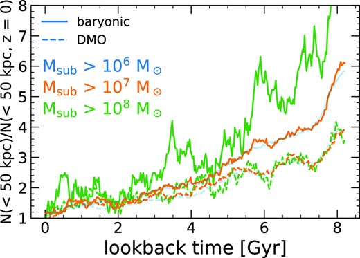
Ratio of the cumulative number of subhaloes enclosed within 50 kpc at varying redshifts to the number at z = 0, as a measure of the relative depletion of subhaloes over cosmic time. Solid lines show the mean across the 11 host haloes, while dashed lines show DMO simulations of the same haloes. Dashed lines for tlb > 5 Gyr show only Latte hosts. We show results for |$M_{\rm sub} \gt 10^{6} \, \text{M}_\odot$| in a lighter shade to indicate potential resolution effects (see Section 2.2). Since z = 1 (tlb ≈ 8 Gyr), the subhalo population in baryonic simulations has decreased by 5 − 10 ×, especially at higher subhalo masses. Subhalo counts at Msub > 108 were as high as 10 × their values today, at tlb ≳ 8 Gyr (extending above the axis).
For use in (semi)analytical models, we fit the three metrics – cumulative number, N(< d), number density, n(d), and orbital flux, f(d) – to the functional form
where a is the expansion scale factor, d is the distance from the MW-mass halo centre, M is the threshold in instantaneous subhalo mass, d0 is a unit normalization of 1 kpc, and |$M_{0} = 10^{7} \, \text{M}_\odot$| is our fiducial mass threshold. Table 3 lists the best-fitting parameters, c0, c1, c2, and c3, for each metric. We generated each of these constants from a particular curve using the Levenberg–Marquardt algorithm: c0 and c3 from Msub > 107 at z = 0 (orange curve in Fig. 1), and c1 and c2 from |$M_\textrm {sub} \gt 10^{7} \, \text{M}_\odot$| at z = 1 (brown curve in Fig. 3). We also fit constant c4 to subhaloes with |$M_{\textrm {sub}} \gt 10^{8} \, \text{M}_\odot$| at z = 0 (green curve in Fig. 1). However, c4 values for all metrics were both very close to one another and very close to previously determined values for the subhalo mass function (Wetzel et al. 2009). In order to reduce the number of constants in the function, we use the median value of our three population metrics, c4 = −0.94, consistent with longstanding expectations for the subhalo mass function. As a metric of uncertainty in our fit, we also include the fractional uncertainty in population amplitude c0, found by taking the product of c0 with the average host-to-host scatter for our fiducial mass range |$M_{\rm sub}\gt 10^{7\ \, \text{M}_\odot }$| at z = 0 (orange curves in Fig. 1).
Fit parameters to equation (1) for subhalo counts and orbital radial fluxes, where a is the expansion scale factor, d is the distance from the MW-mass galaxy in kpc, with d0 = 1 kpc as unit normalization, and M is the lower limit on subhalo instantaneous DM mass in |$\, \text{M}_\odot$|, with |$M_{0} = 10^{7} \, \text{M}_\odot$| as unit normalization. Cumulative number, N(< d) represents the total number of subhaloes enclosed in a sphere of radius d centered on the MW-mass galaxy; number density, n(d), represents the subhalo density in a spherical shell within ±2.5 kpc of d; and radial flux, f(d) represents the number of subhaloes per area that cross into or out of d per Gyr. Accounting for the presence of the LMC (see Section 3.3) boosts these counts by ≈1.4–2.1 ×.
| p(>M, a) | c0 | c1 | c2 | c3 | c4 |
|---|---|---|---|---|---|
| N(<d) | 1.24 ± 0.62 | 12.10 | 2.21 | 1.54 | −0.94 |
| n(d) (kpc−3) | 0.12 ± 0.04 | 10.53 | 1.97 | −1.36 | −0.94 |
| f(d) (Gyr−1 kpc−2) | 8.94 ± 2.82 | 9.08 | 1.48 | −1.10 | −0.94 |
| p(>M, a) | c0 | c1 | c2 | c3 | c4 |
|---|---|---|---|---|---|
| N(<d) | 1.24 ± 0.62 | 12.10 | 2.21 | 1.54 | −0.94 |
| n(d) (kpc−3) | 0.12 ± 0.04 | 10.53 | 1.97 | −1.36 | −0.94 |
| f(d) (Gyr−1 kpc−2) | 8.94 ± 2.82 | 9.08 | 1.48 | −1.10 | −0.94 |
We indicate the distance region used for each fit in Figs 1 and 3 in colour; curves are shown in greyscale outside of this region. We did not use results for |$M_\textrm {sub} \gt 10^{6} \, \text{M}_\odot$| to fit any parameters, given possible limitations from numerical resolution (see Appendix A). However, the dotted lines in Figs 1 and 3 show that our fits for this mass threshold are generally within the 68 per cent host-to-host scatter at d < 50 kpc, reinforcing that any numerical underestimate is likely less than a factor of ≈2.
3.2 Orbital velocity distributions
An essential component for modeling subhalo–stream interactions is the direction of the subhalo orbit relative to the stream (Yoon et al. 2011; Banik et al. 2018). Fig. 5 shows the subhalo orbital velocity components across varying masses and redshifts. The first row shows a metric of the orbital isotropy of the subhalo population, via the ratio of the average absolute radial velocity, |vrad|, to the average tangential velocity, vtan, normalized so that unity represents statistically isotropic orbits. The left three columns show results at z ≈ 0 for our three thresholds in instantaneous mass. The right two columns show subhaloes of |$M_\textrm {sub} \gt 10^{7} \, \text{M}_\odot$| at z ≈ 0.5 and z ≈ 1, as in Fig. 3.
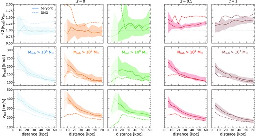
Orbital velocities of subhaloes versus distance, d, from the MW-mass galaxy. Solid lines show the mean, and shaded regions show the 68 per cent distribution across the 11 host haloes, while dashed lines show DMO simulations of the same haloes. Dashed lines for z = 0.5 and z = 1 show only Latte hosts. Lighter shade shows bins where more than 1 halo had an average of 0 subhaloes. Left: subhaloes at z ≈ 0, for Msub > 106, 107, and |$10^{8} \, \text{M}_\odot$|. Right: subhaloes with |$M_\textrm {sub} \gt 10^{7} \, \text{M}_\odot$| at z ≈ 0, 0.5, and 1. Top: Orbital velocity isotropy, via the dimensionless ratio of the median absolute radial velocity to the median tangential velocity, normalized such that isotropic orbits have a value of 1. While subhaloes in DMO simulations have radially biased orbits at all redshifts, subhaloes in baryonic simulations orbit in a nearly statistically isotropic distribution at z ≈ 0. At higher redshifts, subhalo orbits in baryonic simulations were increasingly radially biased. Middle: Median absolute radial velocity, |vrad|. The deepening of the gravitational potential from the MW-mass galaxy in the baryonic simulations increases vrad at small d relative to DMO, but the two are nearly identical at d ≳ 40 kpc. Bottom: Tangential velocity, vtan, is higher in baryonic simulations than in DMO, and this enhancement persists at all d. In addition to the deepening of the gravitational potential, as above, subhaloes with small vtan are more likely to get tidally stripped by the host galaxy and fall below the mass threshold, which further enhances vtan of the surviving population. Thus, subhalo orbits are statistically isotropic at z ≲ 0.5 (tlb ≲ 6 Gyr).
At z ≈ 0, subhaloes in baryonic simulations are consistent with isotropic orbits, in contrast to DMO simulations, in which subhalo orbits are radially biased. Our results suggest that one can approximate a statistically isotropic velocity distribution when modeling and interpreting possible orbits for subhaloes at a given d at z ≈ 0. However, this was not always true: at earlier cosmic times, subhaloes in baryonic simulations were somewhat more radially biased, by up to 1.3× at z = 0.5 and up to 1.4× at z = 1, with larger radial bias at larger d. The DMO simulations also had higher radial bias at earlier times. Most likely, the higher radial bias at earlier cosmic times in both baryonic and DMO simulations arises because subhaloes necessarily fell in more recently, reflecting their initial infall orbits more directly (e.g. Wetzel 2011). Subhaloes that are on highly radial orbits also pass closer to host centre and thus strip/merge more quickly. That said, the reason why the additional gravitational effects of the MW-mass galaxy in the baryonic simulations should lead to a surviving subhalo population with nearly isotropic orbits at z ≈ 0 is not obvious; we defer a more in-depth investigation to future work.
To provide deeper insight into the orbital velocity isotropy, the bottom two rows of Fig. 5 show the individual velocity components, |vrad| and vtan. Beyond ≈40 kpc, |vrad| is similar in both baryonic and DMO simulations. In both, |vrad| increases at smaller d, where the gravitational potential is deeper. However, |vrad| is larger at small d in the baryonic simulations, because the formation of a MW-mass galaxy deepens the potential.
In the bottom row, vtan is higher in baryonic simulations at all d, though again the enhancement is most significant at small d. In addition to the host galaxy deepening the potential, it also provides additional gravitational tidal stripping for subhaloes that orbit close to it, which have small orbital angular momentum, as Garrison-Kimmel et al. (2017) showed. This in turn biases the resultant subhalo population at a given d to have higher vtan. Thus, the stronger enhancement of vtan leads to the change from radially biased orbits in DMO to statistically isotropic orbits in baryonic simulations for surviving subhaloes above a given mass threshold.
At earlier times, both |vrad| and vtan in baryonic simulations were more similar to those in DMO simulations than they are at z ≈ 0, demonstrating how the tidal effects of the host galaxy affected the subhalo population over time. The host galaxy stellar mass increased significantly over this time interval: relative to its stellar mass at z = 0, it typically was only half as large at z = 0.5 and only about a quarter as large at z = 1 (Santistevan et al. 2020; Bellardini et al. 2022).
3.3 Subhalo enhancement during LMC passage
To predict the current subhalo population around the MW, we examine the potential impact of the LMC, a massive satellite galaxy (|$M_\textrm {DM} \sim 10^{11} \, \text{M}_\odot$|) that recently passed its pericentre of 50 kpc (Kallivayalil et al. 2013). We focus on the 4 simulations with LMC satellite analogues in Section 2.3: m12w, m12b, m12f, and m12c.
Fig. 6 shows the subhalo counts over time in each simulation, quantified as the cumulative number of subhaloes within 50 kpc of the MW-mass host, for |$M_{\rm sub} \gt 10^{6} \, \text{M}_\odot$| and |$M_{\rm sub} \gt 10^{7} \, \text{M}_\odot$|. Counts for both mass thresholds visibly increased during the ∼50 Myr after the LMC analog first reached d = 50 kpc, which we indicate with a dotted line. We do not show subhaloes |$\gt 10^{8} \, \text{M}_\odot$| because of their low counts (≲10 subhaloes at any given time) and therefore significant Poisson scatter, but they show similar increases in all four simulations.
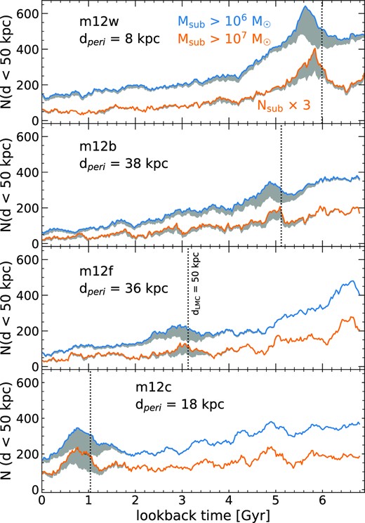
Number of subhaloes within d < 50 kpc of the MW-mass galaxy versus cosmic time, for the 4 simulations that have an LMC satellite analogue. We show subhaloes with instantaneous mass >106 and |$\gt 10^{7} \, \text{M}_\odot$|, with the latter multiplied by 3 for clarity. Grey shaded regions show subhaloes that were satellites of the LMC analogue any time prior to infall. Vertical dotted lines shows when the LMC analogue first orbited within 50 kpc of the MW-mass galaxy, which is the current distance of the LMC from the MW. All four cases show significant enhancement in subhaloes for ≈1–2 Gyr after first infall, after which orbital phase mixing leaves no coherent enhancement during subsequent pericentric passages. Fig. 7 and Table 4 quantify the enhancement of subhaloes during LMC passage.
The grey shaded region indicates the number of subhaloes that ROCKSTAR identifies as having been a satellite of the LMC analogue halo any time before becoming a satellite of the MW-mass halo, demonstrating that this enhancement is primarily (though not entirely) from subhaloes that were satellites of the LMC analogue. This period of subhalo enrichment lasts for only ≲0.5 Gyr after the LMC analog’s first pericentric passage, consistent with previous works that have shown that satellites of LMC-mass satellite galaxies phase mix on this time-scale (e.g. Deason et al. 2015). While some of these additional subhaloes persist indefinitely, the subsequent phase mixing of their orbits leads to no strong temporal enhancement. While these LMC analogs have smaller pericentres about their MW-mass host (8–38 kpc) than the dperi ≈ 50 kpc of the LMC, all four show significant enhancement already when the LMC analog first crosses within d = 50 kpc (vertical dotted line). The latest LMC analogue to reach d = 50 kpc is in m12c at z = 0.07 (tlb = 0.95 Gyr), making it temporally the most similar to the LMC; subhalo counts in this host are 2–4× higher than in the other MW-mass hosts at the same redshift.
Table 4 quantifies the enhancement in the cumulative number and the orbital radial fluxes of subhaloes in our hosts with an LMC satellite analogue via two ratios. The first row compares subhalo counts in each of the four hosts with an LMC analogue at |$t_{\rm 50 ~\text{kpc}}$|, the time at which the LMC analogue first reached d = 50 kpc, to the value in the same host 100–500 Myr earlier. The second row compares subhalo counts in each host with an LMC analogue within ±50 Myr of |$t_{\rm 50 ~\text{kpc}}$| to the average counts in all 11 MW-mass hosts at the same time. We measure cumulative number as in Fig. 1: the total number of subhaloes enclosed within a given distance, in this case |$d=50\ \rm kpc$|. We measure the flux similarly to Fig. 1, now taking the average value of all flux rate data points within the range d = 7.5–50 kpc, representing the flux enhancement over the full range of distances relevant to stellar stream detections. Both the subhalo counts and fluxes increase ≈1.4–2.1×, with broadly consistent enhancement across different mass thresholds. Within R200m, the enhancement in absolute number is much higher (≈100 for |$M_{\rm sub} \gt 10^{7} \, \text{M}_\odot$|) than for d < 50 kpc (≈30), which means that only a fraction of the subhaloes that accreted with the LMC analog contribute to our results at d < 50 kpc. However, the fractional enhancement inside R200m (relative to other hosts at the same time) is weaker than inside d < 50 kpc, being ≈1.1× at all masses, because of the much larger number of preexisting subhaloes within R200m than within d < 50 kpc.
Enhancement of the number and orbital radial flux of subhaloes within 50 kpc of the MW-mass host during 4 LMC satellite analogue events (see Table 2). We measure the subhalo population within ±50 Myr of when each LMC analog first reached d = 50 kpc, and we show the mean and standard deviation of the ratio (as defined below) across these 4 LMC analogue events.Top rows: ratio of each MW-mass halo at the time the LMC analogue reached d = 50 kpc to the average for the same MW-mass halo 100–500 Myr prior, before LMC infall. Subhalo counts and fluxes show a consistent enhancement (1.1–2.3×), so the infall of the LMC analogue significantly boosted the host halo’s subhalo population. Bottom rows: ratio of each MW-mass halo with an LMC analogue to the average of all 11 MW-mass haloes at the same redshift. Subhalo counts and fluxes show similar enhancements (1.4–2.1×).Thus, the MW today likely has a significantly enhanced (≈2×) population of subhaloes relative to similar-mass host haloes today and relative to its own population several 100 Myr ago..
| Subhalo mass threshold (|$\, \text{M}_\odot$|) | Number enhancement | Flux enhancement | |
|---|---|---|---|
| Relative to same MW-mass halo, | >106 | 1.12 ± 0.05 | 1.11 ± 0.12 |
| 100–500 Myr prior | >107 | 1.40 ± 0.08 | 1.37 ± 0.21 |
| >108 | 1.42 ± 0.32 | 1.38 ± 0.59 | |
| Relative to all MW-mass haloes | >106 | 1.41 ± 0.49 | 1.64 ± 0.53 |
| at same redshift | >107 | 1.83 ± 0.72 | 2.00 ± 0.78 |
| >108 | 2.15 ± 1.15 | 1.56 ± 1.16 |
Fig. 7 shows the relative enhancement in subhalo number density, n(d), as a function of d, within our hosts with an LMC analogue within ±50 Myr of |$t_{\rm 50 ~\text{kpc}}$|, compared to all other hosts at the same redshift (as in Table 4, row 2). We find a typical enhancement of ∼1.5–2× at all distances >10 kpc, with relatively weak dependence on both distance and subhalo mass.
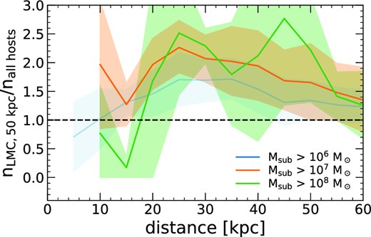
The enhancement of subhaloes around MW-mass galaxies with an LMC satellite analogue. We compute the ratio of the average number density, n(d), of subhaloes around each of the 4 hosts with an LMC satellite analog (m12w, m12c, m12f, and m12b), time-averaged over ±50 Myr when the LMC analog fist crossed within d = 50 kpc, relative to the average across all 11 MW-mass haloes at the same redshift. Shaded regions show the standard deviation across the 4 hosts. MW-mass haloes with an LMC satellite analog show a strong enhancement, typically 1.4 − 2.1×, with only a weak decline with distance..
Given that the LMC is just past its first pericentric passage, our results imply that the MW currently is experiencing a significant boost, typically 1.4–2.1×, in its population of subhaloes at distances ≲50 kpc, both relative to itself a few hundred Myr earlier, and relative to other MW-mass host haloes without an LMC analogue at z = 0. Thus, in making predictions of subhalo counts around the MW today, one should multiply our host-averaged fits in equation (1) by ≈2× (Table 3).
3.4 Predictions for interaction rates with stellar streams
We conclude by synthesizing our results to make approximate estimates for the interaction rates of subhaloes with stellar streams around the MW. To reduce uncertainties from the details of subhalo–stream interaction dynamics, we consider here only near-direct collisions between subhaloes and streams; thus, these values represent conservative estimates of interaction rates.
As case studies, we use the fiducial streams, GD-1 (dperi = 13 kpc, dapo = 27 kpc, length l = 15 kpc) and Pal 5 (dperi = 8 kpc, dapo = 19 kpc, l = 10 kpc), approximating each as a thin cylinder. We use relevant impact parameters (b) for potentially observable subhalo interactions with streams, for each of our three mass thresholds, from Yoon et al. (2011): b < 0.58 kpc for |$M_\textrm {sub} \gt 10^{6} \, \text{M}_\odot$|, b < 1.6 kpc for |$M_\textrm {sub} \gt 10^{7} \, \text{M}_\odot$|, and b < 4.5 kpc for |$M_\textrm {sub} \gt 10^{8} \, \text{M}_\odot$|. These impact parameters come from the tidal radii of subhaloes in each mass bin, thus representing direct subhalo–stream impacts. We then compute the average subhalo flux from our results (Fig. 1, bottom panel) across galactocentric distances corresponding to the orbital ranges of GD-1 (|$13\!-\!27\ \rm kpc$|) and Pal 5 (|$8\!-\!19\ \rm kpc$|). We reiterate that, because subhalo orbits are largely isotropic at z ≈ 0, this radial flux rate can be used as the flux rate in any direction.
We use interaction rates at z < 0.15 (tlb = 0.15 Gyr), and apply an enhancement from the LMC corresponding to the orbital range of each stream, as in Table 4. Under these conditions, for GD-1 we estimate ≈4–5 interactions per Gyr with subhaloes |$\gt 10^{6} \, \text{M}_\odot$|, ≈1–2 per Gyr with |$\gt 10^{7} \, \text{M}_\odot$|, and ≈0–1 per Gyr with |$\gt 10^{8} \, \text{M}_\odot$|; for Pal 5, we estimate ≈2–3 interactions per Gyr with subhaloes |$\gt 10^{6} \, \text{M}_\odot$|, ≈0–1 per Gyr with |$\it \gt 10^{7} \, \text{M}_\odot$|, and ≈0–1 per Gyr with |$\it \gt 10^{8} \, \text{M}_\odot$|. If observable features in streams, such as gaps, persist for many Gyrs, then the evolution across cosmic time is important to incorporate. In this case, we can estimate the ‘effective’ rate by averaging our fluxes across z = 0 − 0.5 (tlb = 0 − 5.1 Gyr), but now omitting the boost factor from the (recently accreted) LMC. For each stream, this increases the interaction rate per Gyr by ≈2 × for Msub > 106 and |$10^{7} \, \text{M}_\odot$|, and up to 4 × for |$M_\textrm {sub} \gt 10^{8} \, \text{M}_\odot$|. Including distant and indirect subhalo–stream encounters, in addition to direct collisions, would further increase these predicted rates.
While only estimates, these encounter rates offer context for our results. Even with the additional tidal effects of the MW-mass galaxy in baryonic simulations, which significantly reduces the population of subhaloes at these distances relative to DMO simulations (down to 10 per cent or fewer from their DMO equivalents), our results imply that, within CDM, interaction rates between stellar streams and dark subhaloes are still sufficient to leave detectable, tidally induced features.
4 SUMMARY AND DISCUSSION
4.1 Summary of results
Using 11 MW-mass host galaxies from the FIRE-2 suite of cosmological simulations, we presented predictions for the counts and orbital distributions of low-mass subhaloes at d ≲ 50 kpc around the MW and MW-mass galaxies. Our primary goal is to inform studies that model potentially observable interactions between such subhaloes and stellar streams. We explored the dependence on subhalo mass, distance, redshift, and the presence of an LMC satellite analogue, and we provided analytical fits to these dependencies.
Our primary results are:
The incorporation of baryonic physics significantly reduces subhalo counts compared with DMO simulations, primarily because of additional tidal force from the MW-mass galaxy potential. At z ≈ 0, DMO simulations overpredict subhalo counts by ≈4–5 times at d ≈ 20 kpc. These differences were less pronounced at earlier cosmic times, with DMO simulations overpredicting counts by ≈1.5 times at z = 0.5.
We predict that >20 (>4) subhaloes with instantaneous mass|$\gt 10^{6} \, \text{M}_\odot$| (|$\gt 10^{7} \, \text{M}_\odot$|) exist within the distances of streams like GD-1 and Pal 5 (d ≲ 30 kpc), and at least 1 subhalo |$\gt 10^{8} \, \text{M}_\odot$| resides within d < 50 kpc. Thus, despite the strong depletion of subhaloes in baryonic simulations relative to DMO, significant numbers of subhaloes survive at the distances of observed stellar streams. This is unlike Garrison-Kimmel et al. (2017), who found no surviving subhaloes within ≈15 kpc, but they only examined two of these FIRE-2 simulations (m12i, m12f) at a single snapshot at z = 0.
At z ≈ 0, subhalo number density and orbital flux are nearly constant with distance, out to at least d ≈ 60 kpc.
Subhalo counts decreased significantly over cosmic time, from both the declining rate of infall of new subhaloes and the increasingly strong tidal field of the host galaxy. At z = 1, the MW-mass hosts had ≈10 times more subhaloes at a given distance. This decline over time is stronger at smaller distances and at higher subhalo masses.
Subhaloes orbit with statistically isotropic velocities at z ≈ 0 but they were increasingly radially biased at earlier times. This is unlike DMO simulations, in which subhalo orbits are always radially biased. That subhalo velocities are isotropic at z ≈ 0 implies that our subhalo radial flux values can also be applied to subhalo flux in any desired direction.
The initial infall of an LMC satellite analog boosts the number of subhaloes within 50 kpc of the MW-mass host by 1.4–2.1 times, relative to the same host a few hundred Myr earlier or relative to similar-mass host haloes at the same time. Thus, predictions and models for subhalo-stream interaction rates over the last few 100 Myr should take into account this enhancement from the LMC.
4.2 Discussion
As expected, we find similar overall results as Garrison-Kimmel et al. (2017), who examined two of the same FIRE-2 haloes as we do (m12i, m12f). However, we emphasize key differences and extensions of our work compared with theirs. First, we include more host haloes (11) for better statistics. Second, and equally importantly, we time-averaged our results across multiple snapshots. Given our snapshot time spacing of 20–25 Myr, this provides a much more statistically representative picture of subhaloes at small distances, where their velocities are highest and where they spend the least time in their orbit. Furthermore, we interpolate subhalo distances between snapshots (see Section 2.2) to avoid missing orbits at particularly small distances. Unlike Garrison-Kimmel et al. (2017), who found no surviving subhaloes within ≈15 kpc of m12i and m12f at z = 0, we find that subhaloes survive, if briefly, at all d ≳ 5–10 kpc at all mass thresholds.
We next discuss caveats to our results. While we selected these host galaxies/haloes for their similarity to the MW, they are not exact analogues. Each one has a different formation and merger history, resulting in significant host-to-host variation (Santistevan et al. 2020). In general, we averaged our results across these 11 hosts and included the host-to-host scatter, to present cosmologically representative results for subhaloes around MW-mass galaxies. This is statistically likely to encompass the population around the MW, but there is no guarantee of it. We compared our results for our isolated haloes to our Local Group analogues and found negligible differences, consistent with the comparisons among the ELVIS DMO simulations in Wetzel, Deason & Garrison-Kimmel (2015), indicating that such environmental selection is not a significant factor affecting these low-mass subhaloes at distances ≲50 kpc.
More critically, our results demonstrate that the presence of an LMC satellite analogue boosts low-mass subhalo counts by 1.4–2.1× at distances ≲50 kpc (Table 4), indicating that this is one of, and likely the, most important factor in predicting subhalo populations around the MW today and over the last few 100 Myr. All of our LMC analogues have smaller pericentres than the LMC, ranging from 8 to 38 kpc. We mitigated this by measuring subhaloes when the LMC analogue first cross within the LMC’s current pericentric distance of ≈50 kpc. Arora et al. (in preparation) examine subhalo populations in selected hosts of the FIRE-2 simulations at different angular locations around the galactic centre, including the spatial relation to LMC analogues, as well as specific subhalo-stream encounter rates in the presence of a massive satellite.
We examined results only for one DM model, CDM, but there are many other possible candidates. Extensions of our work would include examining FIRE simulations with alternative DM models (such as Robles et al. 2017; Shen et al. 2022).
As with any simulation, our results are susceptible to resolution effects. We reiterate that, motivated by quantifying the strength of gravitational interactions with stellar streams, we selected subhaloes above a given instantaneous threshold in mass, so numerical convergence requires that our simulations accurately model the amount of mass stripping in subhaloes down to our given instantaneous mass threshold(s). Thus, our results are not sensitive to modeling any mass stripping (physical or numerical) that occurs below this threshold, or to the more challenging question of modeling/defining subhalo ‘disruption’, which occurs below these mass thresholds.
In Appendix A, we quantify resolution convergence by comparing our fiducial subhalo counts to those in both lower resolution and higher resolution versions of the same haloes. To summarize, our tests indicate that subhalo counts at instantaneous |$M_\textrm {sub} \gt 10^{7} \, \text{M}_\odot$| are reasonably well converged, but at |$M_\textrm {sub} \gt 10^{6} \, \text{M}_\odot$| our simulations underpredict the counts by up to ≈1.5–2 × (which we have indicated throughout), so our results there are lower limits, which means that the actual interaction rates with streams would be even higher. And again, in fitting our results, we did not include any values at |$M_\textrm {sub} \gt 10^{6} \, \text{M}_\odot$|, so our fit values there are extrapolations from our higher masses.
We also discuss the numerical convergence of our subhaloes in the context of the criteria that van den Bosch & Ogiya (2018) provided from idealized simulations of individual subhaloes orbiting in fixed host halo potential without a central disc. They consider a subhalo to be sufficiently resolved based on its bound mass fraction, fbound, the ratio of its instantaneous mass to its peak mass (typically just before accretion), with a minimum fbound determined by the subhalo’s scale radius, rs,0, and the number of DM particles it had at its peak mass, Npeak. They define |$f_{\rm bound}^{\rm min,1} = C \left(\epsilon /r_{\rm s,0} \right)^{2}$| and |$f_{\rm bound}^{\rm min,2} = 0.32 \left(N_{\rm peak}/1000 \right)^{-0.8}$|, where C is a constant that depends on the subhalo’s concentration parameter (we use C ≈ 10, based on their section 6.4), ϵ is the Plummer force softening of the simulation, which is 40 pc for all of our simulations, and Npeak is the peak number of constituent DM particles a subhalo experienced, typically prior to accretion. Bosch & Ogiya (2018) consider a subhalo converged if it satisfies both criteria, that is, |$f_{\rm bound}^{\rm min} = \textrm {MAX}(f_{\rm bound}^{\rm min,1},f_{\rm bound}^{\rm min,2})$|.
For reference, we note the median values for these relevant quantities for each of our subhalo samples at z = 0. For |$M_{\rm sub} \gt 10^{6} \, \text{M}_\odot$| (1436 subhaloes), the median |$M = 2.4 \times 10^{6} \, \text{M}_\odot$|, |$M_{\rm peak} = 1.3 \times 10^{7} \, \text{M}_\odot$|, rs,0 = 0.15 kpc, and Npeak = 517. For |$M_{\rm sub} \gt 10^{7} \, \text{M}_\odot$| (209 subhaloes), the median |$M = 2.9 \times 10^{7} \, \text{M}_\odot$|, |$M_{\rm peak} = 8.5 \times 10^{7} \, \text{M}_\odot$|, rs,0 = 0.18 kpc, and Npeak = 3419. For |$M_{\rm sub} \gt 10^{8} \, \text{M}_\odot$| (13 subhaloes), the median |$M = 2.3 \times 10^{8} \, \text{M}_\odot$|, |$M_{\rm peak} = 8.2 \times 10^{8} \, \text{M}_\odot$|, rs,0 = 1.5 kpc, and Npeak = 39, 461. For all mass thresholds, the median fbound ≈ 0.26, that is, all samples have experienced the same typical fraction of mass stripping since Mpeak.
Applying the convergence criterion from Bosch & Ogiya (2018) to our samples, for Msub > 106, >107, and |$\gt 10^{8} \, \text{M}_\odot$|, the fraction of subhaloes that meet the criterion for mass resolution, |$f_{\rm bound}^{\rm min,2}$|, is 17, 92, and 100 per cent, respectively. The criterion for spatial resolution, |$f_{\rm bound}^{\rm min,1}$|, is more stringent. Enforcing both |$f_{\rm bound}^{\rm min,1}$| and |$f_{\rm bound}^{\rm min,2}$| brings these fractions down to 6, 39, and 69 per cent. Nearly all subhaloes at Msub > 107 and |$10^{8} \, \text{M}_\odot$| had |$f_{\rm bound} \gt f_{\rm bound}^{\rm min,2}$| (92 and 100 per cent, respectively), so |$f_{\rm bound}^{\rm min,1}$| dominates this population’s convergence fraction. In agreement with our resolution tests, the convergence fraction for |$M_{\rm sub} \gt 10^{6} \, \text{M}_\odot$| is significantly lower.
However, the idealized simulations in Bosch & Ogiya (2018) did not include a central disc potential, which significantly increases the physical tidal force and therefore mass stripping at d ≲ 50 kpc. This may relax the criteria on |$f_{\rm bound}^{\rm min}$|; for example, in an extreme limit of a strong tidal field that induces (nearly) complete physical mass stripping at first pericentre, numerical considerations of resolving subhaloes above a given instantaneous mass threshold across many orbits become less significant. Webb & Bovy (2020) also explored the effects of resolution on simulated subhaloes, using re-simulations taken from the Via Lactea II simulation, and they also included an MW-mass disc potential. They found that subhaloes with |$M_{\rm sub} \sim 10^{7} \, \text{M}_\odot$| at the resolution and force softening lengths of our FIRE-2 simulations can lose up to 60 per cent of their mass over the course of their lifetimes (across up to ∼5 Gyr) relative to their counterparts at higher resolution, while subhaloes at |$M_{\rm sub} \sim 10^{6} \, \text{M}_\odot$| dissipate entirely. Though, their static host galaxy potential had higher mass at earlier times than our cosmological simulations: over the last 5 Gyr, the central galaxy in our simulations increased by typically ≈30 per cent. Additionally, individual subhaloes exhibit a wide range of infall times; since most mass-loss occurs during infall, subhaloes with later infall times are subject to artifical mass-loss effects for a shorter period of time. Santistevan et al. (2023) examined the infall times of luminous satellites in the same simulations, finding a 68th percentile range of 4–10 Gyr at the low subhaloes masses that we analyse here. We reiterate that our convergence tests in Appendix A provide the most direct numerical test of our cosmological setup.
Comparing with previous works, our results generally agree with those that modeled an MW-mass galaxy potential. Compared to D’Onghia et al. (2010), who examined subhaloes in the Aquarius DMO simulation with an added galaxy disc potential, we find the same order-of-magnitude results for |$M_\textrm {sub} \gt 10^{6} \, \text{M}_\odot$| (their counts being ≈2.5× higher than ours within d = 50 kpc, and approximately the same as ours within d = 20 kpc), but lower counts for |$M_\textrm {sub} \gt 10^{8} \, \text{M}_\odot$| (≈4× within d = 50, ≈20× within d = 20 kpc). Other works that compared subhalo populations in DMO simulations to those that also model a central galaxy potential found that DMO simulations overpredict subhaloes at d ≲ 50 kpc by ≈1.5× (D’Onghia et al. 2010), ≈1.8× (Garrison-Kimmel et al. 2017), ≈3.3× (Kelley et al. 2019), and ≈3× (Nadler et al. 2021). By, comparison, we find ≈2–3×, on average, with some dependence on subhalo mass. Additionally, Webb & Bovy (2020) found that, broadly speaking, DMO simulations overpredict the entire subhalo population within an MW-mass halo by a factor of ≈1.6, in broad agreement with our simulations, which have a mean DMO excess of 1.56 for subhaloes with |$M_{\rm sub} \gt 10^{7} \, \text{M}_\odot$| at z = 0.
This reinforces that the most important effect of baryons for low-mass subhaloes is simply the addition of the tidal field from the central galaxy, as Garrison-Kimmel et al. (2017) demonstrated by showing similar results for the FIRE-2 baryonic simulations compared with simply adding a central galaxy potential to DMO simulations of the same haloes. This agreement supports the use of an embedded central galaxy potential in DMO simulations as a computationally inexpensive alternative to simulations with full baryonic physics. Furthermore, if using existing DMO simulations (e.g. as in Hargis et al. 2014; Griffen et al. 2016), one can increase the accuracy of subhalo counts by reducing them using the distance-dependent correction fits from Samuel et al. (2020), which agree with our results, or using the machine-learning approach to subhalo orbital histories, as in Nadler et al. (2018).
Sawala et al. (2017) examined subhaloes of instantaneous mass |$10^{6.5}\!-\!10^{8.5} \, \text{M}_\odot$| in the APOSTLE simulations of Local Group analogs (DM particle mass |$\approx 10^{4} \, \text{M}_\odot$|, force softening ≈134 pc); we find broadly similar subhalo counts for both |$M_\textrm {sub} \gt 10^{7} \, \text{M}_\odot$| (within ≈1.4 × of our counts) and |$\gt 10^{8} \, \text{M}_\odot$| (within ≈1.5 × of our counts) at d = 50 kpc. Sawala et al. (2017) also compared their results to DMO versions of the same simulations and found similar DMO overpredictions of ≈2 × at d = 50 kpc for |$M_\textrm {sub} \gt 10^{7} \, \text{M}_\odot$|, with more dramatic DMO overprediction than our results at smaller distances (≈4× at d = 20 kpc). However, the typical central galaxy in APOSTLE has significantly lower stellar mass, with |$M_{\rm star} \approx 1.8 \times 10^{10} \, \text{M}_\odot$|, compared to our typical |$M_{\rm star} \approx 6 \times 10^{10} \, \text{M}_\odot$|, which is similar to the MW. We also note similar trends in subhalo tangential and radial velocities, although subhalo orbits are generally less isotropic at small distances.
Zhu et al. (2016) compared a baryonic versus DMO version of the Aquarius simulation, finding that DMO overpredicts subhaloes by ≈3× at |$M_{\rm sub} \gt 10^{7} \, \text{M}_\odot$| and ≈4–5× at |$M_{\rm sub}\gt 10^{8} \, \text{M}_\odot$| within the host halo’s radius. The larger-volume, lower-resolution Illustris and EAGLE simulations also demonstrate similar general trends of subhalo depletion in baryonic relative to DMO versions at small distances (e.g. Chua et al. 2017; Despali & Vegetti 2017).
We also compare to previous work that used simulations to predict subhalo populations and subhalo-stream interaction rates. Our estimates for interaction rates (Section 3.4) are similar to those of Yoon et al. (2011), who used a lower resolution DMO halo, designed to be similar to the MW’s, with an added stream, predicted the Pal 5 stream to have ≈20 detectable subhalo-induced gaps. Banik et al. (2018) simulated the evolution of GD-1 near a MW potential and estimated that the MW hosts ≈0.4× the number of subhaloes in a comparable DMO simulation, generally consistent with our results (Fig. 2).
To conclude, we presented cosmological predictions for subhalo counts and orbital fluxes (Figs 1 and 3) as well as velocity distributions (Fig. 5), and we provided fits to these results, to inform studies that seek to predict and interpret observable effects of subhalo gravitational interactions on stellar streams.
ACKNOWLEDGEMENTS
We thank Adrian Price-Whelan for suggesting that we explore the effect of the LMC on predictions for subhalo populations. We thank Isaiah Santistevan, Pratik Gandhi, and Nicolas Garavito for helpful comments and discussion. We also thank the anonymous referee for providing helpful and insightful comments and feedback. MB and AW received support from: National Science Foundation (NSF) via CAREER award AST-2045928 and grant AST-2107772; National Aeronotics and Space Administration (NASA) Astrophysics Theory Program (ATP) grant 80NSSC20K0513; Hubble Space Telescope (HST) grants AR-15809, GO-15902, GO-16273 from Space Telescope Science Institute (STScI). We completed this work in part at the Aspen Center for Physics, supported by NSF grant PHY-1607611. We ran simulations using: eXtreme Science and Engineering Discovery Environment (XSEDE), supported by NSF grant ACI-1548562; Blue Waters, supported by the NSF; Frontera allocations AST21010 and AST20016, supported by the NSF and Texas Advanced Computing Center (TACC); Pleiades, via the NASA HEC program through the NASA Advanced Supercomputing (NAS) Division at Ames Research Center. We used numpy (Harris et al. 2020), scipy (Jones et al. 2001), astropy (Astropy Collaboration 2018), and matplotlib (Hunter 2007), as well as the publicly available package HaloAnalysis (Wetzel & Garrison-Kimmel (2020c), available at https://bitbucket.org/awetzel/halo_analysis/).
DATA AVAILABILITY
The data in these figures and all of the python code that we used to generate these figures are available at the following repository: https://bitbucket.org/meganbarry/subhalos_2023/. FIRE-2 simulations are publicly available (Wetzel et al. 2023) at http://flathub.flatironinstitute.org/fire. Additional FIRE simulation data is available at https://fire.northwestern.edu/data. A public version of the gizmo code is available at http://www.tapir.caltech.edu/~phopkins/Site/GIZMO.html.
References
APPENDIX: RESOLUTION CONVERGENCE
Here, we examine the resolution convergence of our counts for subhaloes that we select above a given instantaneous threshold in mass. Thus, our tests are sensitive to how well the simulations model the correct amount of mass stripping that occurs down to a given instantaneous threshold in subhalo mass, but our results are not sensitive to mass stripping or ‘disruption’ (physical or numerical) that occurs below that threshold.
We pursue two convergence tests. First, we compare our fiducial-resolution (FR) simulations against a suite of lower-resolution (LR) re-simulations of the same haloes. We simulated each halo in the Latte suite at 8 times lower mass resolution and 2 times larger force softening. Thus, subhaloes with |$M_{\rm sub} \gt 8 \times 10^{6} \, \text{M}_\odot$| and |$M_{\rm sub} \gt 8 \times 10^{7} \, \text{M}_\odot$| in the LR simulations have the same number of DM particles as those at |$M_{\rm sub} \gt 10^{6} \, \text{M}_\odot$| and |$\gt 10^{7} \, \text{M}_\odot$| in the FR simulations, so comparing counts at |$M_{\rm sub} \gt 8 \times 10^{6} \, \text{M}_\odot$| and |$\gt 8 \times 10^{7} \, \text{M}_\odot$| provides a convergence test of our fiducial results at fixed number of DM particles (though the force softenings in LR simulations are also 2× larger). We do not test counts at |$M_{\rm sub} \gt 8 \times 10^{8} \, \text{M}_\odot$|, because their small numbers lead to significant Poisson noise.
Fig. A1 shows subhalo number density, n(d) (as defined in Section 2.2), as a function of distance from the host galaxy, d, time-averaged over the same 92 snapshots at z ≈ 0 as in Fig. 1.
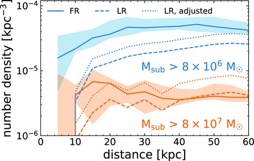
Resolution convergence test of subhalo number density, n(d), versus distance from MW-mass galaxy, d, for FR and LR simulations of the same 6 haloes in the Latte suite, time-averaged over the same 92 snapshots as Fig. 1. LR simulations have 8 × larger particle masses and 2 × larger force softening. We show the average n(d) and host-to-host scatter for |$M_{\rm sub} \gt 8 \times 10^6 \, \text{M}_\odot$| and |$\gt 8 \times 10^7 \, \text{M}_\odot$|, which correspond to the same number of particles in the LR simulations as for our fiducial mass thresholds of |$\gt 10^6 \, \text{M}_\odot$| (≈30 particles) and |$\gt 10^7 \, \text{M}_\odot$| (≈300 particles) in the FR simulations. Dotted lines show ‘adjusted’ counts in the LR simulations to correct for them forming more massive host galaxies that induce stronger tidal stripping (see text). For subhaloes at |$\gt 8 \times 10^{7} \, \text{M}_\odot$|, n(d) for LR and LR adjusted bracket and largely fall within the 68 per cent scatter of the FR simulations, especially at d ≈ 15 − −35 kpc. By contrast, the LR simulations underpredict subhalo counts at |$\gt 8 \times 10^{6} \, \text{M}_\odot$| by a factor of ≈2. These results indicate that, in our FR simulations, subhalo counts at |$M_{\rm sub} \gt 10^{7} \, \text{M}_\odot$| are reasonably well converged but subhalo counts at |$\gt 10^{6} \, \text{M}_\odot$| are lower limits.
One complication to this comparison is that the LR simulations form host galaxies with higher (≈1.7× on average) stellar mass (see Hopkins et al. 2018; Samuel et al. 2020), resulting in an increased tidal force and stripping on subhaloes (in addition to resolution effects). Following Samuel et al. (2020), we determine a correction factor for the subhalo count in the LR simulation, which we show as a dotted line (LR, adjusted). Specifically, we fit a power law to the relation between |$N_{\rm sub}(\lt 50\, \textrm {kpc})$| and host M⋆ at each threshold in subhalo mass. This fit indicates that, at fixed resolution, a host galaxy with 1.7× larger stellar mass has 0.73 (0.58) times as many subhaloes at |$\gt 8 \times 10^{6} \, \text{M}_\odot$| (|$\gt 8 \times 10^{7} \, \text{M}_\odot$|). Once we correct for the discrepancy in host galaxy mass, the subhalo counts at |$M_\textrm {sub} \gt 8 \times 10^{7} \, \text{M}_\odot$| agree reasonably well, within the host-to-host scatter, especially at 15 − −35 kpc, with a slight depletion at smaller d and excess at larger d. Counts for subhaloes at |$\gt 8 \times 10^{6} \, \text{M}_\odot$| are lower by a factor of ≈2 in the LR simulations (adjusted for host galaxy mass) at all d, indicating that resolution effects are more important at this mass threshold. Thus, as we emphasize throughout, we interpret predictions from our FR simulations at |$M_\textrm {sub} \gt 10^{6} \, \text{M}_\odot$| to be lower limits. See Samuel et al. (2020) for similar convergence tests comparing subhaloes at fixed peak mass (instead of instantaneous mass).
Second, for the single host halo m12i, we also compare our fiducial results against an ultra-high-resolution (UHR) version simulated to z = 0 (Wetzel et al., in preparation), for both baryonic and DMO simulations. This UHR simulation has 8 × smaller DM particle mass (|$4400 \, \text{M}_\odot$|) and 2 × smaller DM force softening (20 pc). Fig. A2 shows subhalo n(d) versus d, comparing FR and UHR, for m12i at z ≈ 0, time-averaged across the same 92 snapshots. In this case, the host galaxy forms the same stellar mass in both simulations, so we do apply any adjustment as in Fig. A1. Number density at both resolutions is now similar for both |$\gt 10^{6} \, \text{M}_\odot$| and |$\gt 10^{7} \, \text{M}_\odot$|, to within the snapshot-to-snapshot scatter.
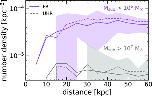
Resolution convergence test of subhalo number density, n(d), versus distance from host halo centre, d, for a single halo, m12i, time-averaged over the same 92 snapshots at z ≈ 0 as Fig. 1. We compare against re-simulations of m12i at UHR, with 8× better mass resolution and 2× better force resolution than FR (Wetzel et al., in preparation). The shaded region shows the 68 per cent scatter across the 92 snapshots for our fiducial resolution. Compared to Fig. A1, we find better convergence between the two simulations as resolution increases, with differences between FR and UHR for |$M_\textrm {sub} \gt 10^{6} \, \text{M}_\odot$| being a factor of only ≈1.1×.
Taken together, Figs A1 and A2 imply that our FR simulations, which we presented throughout, have reasonably converged subhalo counts at |$\gt 10^{7} \, \text{M}_\odot$|, but they underpredict subhalo counts at |$M_\textrm {sub} \gt 10^{6} \, \text{M}_\odot$| by up to ≈1.5 − −2×.
