


ABSTRACT
Tsinghua University-Ma Huateng Telescope for Survey (TMTS) aims to discover rapidly evolving transients by monitoring the northern sky. The TMTS catalogue is cross-matched with the white dwarf (WD) catalogue of Gaia EDR3, and light curves of more than a thousand WD candidates are obtained so far. Among them, the WD TMTS J23450729+5813146 is one interesting common source. Based on the light curves from the TMTS and follow-up photometric observations, periods of 967.113, 973.734, 881.525, 843.458, 806.916, and 678.273 s are identified. In addition, the TESS observations suggest a 3.39-h period but this can be attributed to the rotation of a comoving M dwarf located within 3 arcsec. The spectroscopic observation indicates that this WD is DA type with Teff = 11 778 ± 617 K, log g = 8.38 ± 0.31, mass = 0.84 ± 0.20 M⊙, and age = 0.704 ± 0.377 Gyr. Asteroseismological analysis reveals a global best-fitting solution of Teff = 12 110 ± 10 K and mass = 0.760 ± 0.005 M⊙, consistent with the spectral fitting results, and oxygen and carbon abundances in the core centre are 0.73 and 0.27, respectively. The distance derived from the intrinsic luminosity given by asteroseismology is 93 parsec, which is in agreement with the distance of 98 parsec from Gaia DR3. Additionally, kinematic study shows that this WD is likely a thick-disc star. The mass of its zero-age main sequence is estimated to be 3.08 M⊙ and has a main sequence plus cooling age of roughly 900 Myr.
1 INTRODUCTION
In our Milky Way, up to 97 per cent of all stars will eventually evolve into white dwarfs (WDs; Heger et al. 2003). Main-sequence stars with masses no more than 10–11 M⊙ (Woosley & Heger 2015) will end up as WDs, depending on their metallicity as well. WDs are objects of great importance that can provide vital information in a variety of research fields (Althaus et al. 2010). Owing to a simple cooling mechanism, it is easier to derive relatively accurate ages of WDs, making them suitable for studies on the ages of Galactic populations (Guo et al. 2019; Kilic et al. 2019), which are important tools by studying their luminosity functions (Munn et al. 2017; Lam et al. 2019) and mass functions (Holberg et al. 2016; Hollands et al. 2018). Accurate WD luminosity functions can be adopted to infer the structure and evolution of the Galactic disc and open and globular clusters (Bedin et al. 2009; Campos et al. 2016; García-Berro & Oswalt 2016; Kilic et al. 2017; Guo et al. 2018). Furthermore, massive carbon–oxygen WDs are progenitors of Type Ia supernovae (SNe Ia), which serve as standard candles for cosmological studies (Maoz, Mannucci & Nelemans 2014). Ultra-short period double WDs are potential gravitational wave sources likely to be detected by space gravitational wave facilities like Laser Interferometer Space Antenna (LISA, Burdge et al. 2019).
With large spectroscopic surveys like Palomar-Green (Green, Schmidt & Liebert 1986), Sloan Digital Sky Survey (SDSS, York et al. 2000), and Large Sky Area Multi-Object Fiber Spectroscopic Telescope (LAMOST, Zhao et al. 2012), the studies of WDs have entered a new era by increasing the numbers of WDs greatly (Kleinman et al. 2013; Zhao et al. 2013; Gentile Fusillo et al. 2015; Guo et al. 2015b, 2022; Kepler et al. 2015, 2019; Kong & Luo 2021). Thanks to the Gaia mission (Gaia Collaboration 2016), the studies of WD now step into another new era. With the release of early Gaia DR3, the number of WDs reached ∼359 000 (Gentile Fusillo et al. 2021). This catalogue is extremely helpful for studying light variability of WDs by cross-matching it with some photometric surveys.
Asteroseismology makes the studies of internal structure of pulsating stars become possible. This is also true for the studies of pulsating WDs (see a recent review by Córsico et al. 2019). Since the first discovery of pulsating DA WD (DAV or ZZ ceti) HL Tau 76 (Landolt 1968), there are as many as 494 DAVs identified via photometric observations (Córsico 2022), including those discovered with TESS (Romero et al. 2022). Many of those DAVs have been analysed with asteroseismology from different groups using different models and asteroseismic approaches. Among them, two main methods are widely adopted. One uses static stellar models with parametrized chemical profiles. It allows a full exploration of the parameter space to find an optimal seismic model, leading to good matches to the observed periods. (Bradley 1998, 2001; Bischoff-Kim, Montgomery & Winget 2008; Castanheira & Kepler 2009; Bischoff-Kim & Metcalfe 2011; Bischoff-Kim et al. 2014; Giammichele et al. 2017a, b). Another approach is using full evolutionary models, which is generated by tracking the full evolution of the progenitor star, from the zero-age main sequence (ZAMS) to the WD stage (Romero et al. 2012, 2013; Córsico et al. 2013; De Gerónimo et al. 2017, 2018). It has been shown that detailed analysis on individual DAV is needed to understand the precise parameters of the WD stars. In return, models can be improved based on observations. In general, the instability strip of DAVs is in the range of 10 850 and 12 270 K (Gianninas, Bergeron & Ruiz 2011), and the atmospheres of these cool WDs are almost dominated by pure hydrogen as a result of gravitational settling of other heavier elements. The hydrogen in the outer envelope recombines at around |$T_{\rm eff}\sim 12\, 000$| K, which causes a huge increase in envelope opacity. Consequently, this restrains the flow of radiation and eventually results in g-mode oscillations (Winget et al. 1982). Owing to the fact that these oscillation-induced pulsation modes are very sensitive to the stellar structure of DAVs, they can be used to study the internal structures of these stars.
Over the past decade, the Kepler (Borucki et al. 2010) and its K2 mission (Howell et al. 2014) have made high-precision asteroseismology of WDs possible (Hermes et al. 2011; Greiss et al. 2016). Later, the TESS mission (Ricker et al. 2015) has enriched the sample, as it observes the whole sky (Campante et al. 2016; Romero et al. 2022). However, Kepler and K2 mainly focus on specific areas, while TESS will cover the whole sky area, but its size is too small for faint objects. Therefore, ground-based survey telescope with short cadence is still vital for discovery and asteroseismological study of faint pulsating WDs.
In this work, we report our discovery and results of asteroseismological analysis of a new DAV star TMTS J23450729+5813146 (dubbed as J2345) discovered by Tsinghua University-Ma Huateng Telescope for Survey (TMTS). This star, with coordinates of RA = 23:45:07.29 and Dec. = +58:13:14.6, was first reported in Gaia DR2 WD catalogue as a WD candidate with a probability being WD PWD = 0.99 and G = 16.88 mag (Gentile Fusillo et al. 2019). Through spectral energy distribution (SED) fitting to hydrogen-rich and helium-rich atmosphere models, the parameters of J2345 are estimated to be Teff = 11 280 K, log g = 8.04, and mass = 0.63 and Teff = 11 069 K, log g = 7.93, and mass = 0.54, respectively. Then, it was studied in Gaia 100 pc infrared-excess WD sample (Rebassa-Mansergas et al. 2019), as it seems to comove with a nearby faint (G = 19.15 mag) M star. In their paper, the effective temperature of J2345 and the companion are estimated to be 11 750 and 2800 K, respectively, via SED fitting. No public spectrum data are available for J2345 so far.
This paper is arranged as follows: In Section 2, observational details of J2345 are listed. In Section 3, frequency solution and asteroseismological modelling of J2345 are presented. Period from TESS is analysed in Section 4, while discussions and summary are given in Sections 5 and 6, respectively.
2 OBSERVATIONS
2.1 TMTS
TMTS is a photometric survey with four 40-cm optical telescopes, located at Xinglong station in China. It has a total field of view of ∼18 deg2 (4.5 deg2 each) and equipped with four 4k × 4k pixels CMOS cameras, which allow less than a second read-out time and high-speed photometry. The survey operates in two observation modes: first, uninterrupted observing LAMOST areas for the whole night with a cadence of 1 min, carrying out collaborative tasks with the LAMOST, and secondly, SN survey with a cadence of 1–2 d. For the purpose of reaching out the full potential of observations, customized filter covering 330–900 nm is used for the survey. The 3σ detection limit of TMTS can reach 19.4 mag for 1-min exposure. More description regarding the performance of TMTS can be found in Zhang et al. (2020) and Lin et al. (2022a, b).
TMTS started the 1-min-cadence survey in 2020, producing uninterrupted light curves for more than 10 million objects so far. The WD catalogue generated from Gaia EDR3 (Gentile Fusillo et al. 2021) is used to cross-match with the TMTS catalogue within 3 arcsec, which yields more than a thousand WD common sources. Based on visual inspections of each source, WD J2345 was selected as a pulsating WD candidate for detailed study. WD J2345 was observed by TMTS on two nights (see details in Table 1). A part of the discovery light curve is shown in Fig. 1. The amplitude of variation is large for a ZZ ceti, roughly 0.2–0.3 mag.
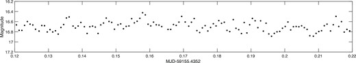
A part of the discovery TMTS light curve taken on 2020 December 2. The amplitude of variation is large for a DAV.
Observation logs of J2345.
| Telescope | Instrument | Obs_date | Exposure (s) |
|---|---|---|---|
| TMTS | CMOS | 2020-11-01 | 60 |
| (4 × 40 cm) | (330–900 nm) | 2020-11-02 | 60 |
| SNOVA (40 cm) | CCD | 2021-11-07 | 50 |
| (White light) | 2021-11-08 | 100 | |
| 2021-11-10 | 100 | ||
| 2021-11-11 | 100 | ||
| 2021-11-14 | 100 | ||
| Shane (3 m) | Kast Double | 2021-11-07 | 3600 |
| Spectrograph | 2021-11-12 | 2400 | |
| TESS | CCD | 2019/Sector17 | 120/1800 |
| (600–1000 nm) | 2020/Sector24 | 120/1800 |
2.2 Spectral observations
Spectral follow-up observations have been carried out by 3-m Shane telescope located at Lick observatory in 2021. Both spectra were taken by Kast double spectrograph with a slit width of 2 arcsec and grism 2, covering 3600–5700 Å in blue and 5400–10 760 Å in red, providing a spectral resolution of roughly 1.02 Å per pixel. The standard procedures of dark current subtraction, bias subtraction, cosmic ray removal, and 1D spectral extraction are performed using iraf. The signal-to-noise ratio (SNR) of the spectrum taken on 12 November is much better than the other due to better seeing; thus, only the spectrum with higher SNR is used for spectral analysis. Owing to its higher SNR, blueshifted lines are noticeably seen in the spectrum. Spectral fitting with WDTOOLS (Chandra 2020; Chandra et al. 2020) yields a radial velocity of −67.7 ± 17.2 km s−1. After corrections for the line shift, the parameters of J2345 are derived as Teff = 11 778 ± 617 K, log g = 8.38 ± 0.31, mass = 0.84 ± 0.20 M⊙, and age = 0.704 ± 0.377 Gyr, based on the spectral model fitting method described in Guo et al. (2015b, 2022). The spectrum and best fit are shown in Fig. 2. The derived Teff and mass are especially helpful for providing independent check of the results from asteroseismological analysis.
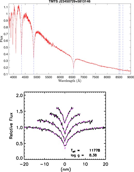
Spectrum taken by Lick 3-m Shane telescope and its spectral fitting. From left to right, blue dashed lines in the upper panel mark the Hγ, Hβ, Hα, and Ca ii triplet lines, respectively. From bottom to top, black lines in the lower panel are normalized Hα, Hβ, Hγ, and Hϵ lines, respectively. Red dashed lines are the best model fitting after corrections for blueshift.
2.3 Photometric follow-up
Additional follow-up photometric observations have been taken by a 40-cm telescope called SNOVA located at Nanshan station in China. A total of five nights observations have been taken for J2345. All these observations are observed in white light with an exposure time of approximately 100 s. The standard image processing, like bias correction, flat correction, and source extraction, is performed with iraf, and then differential photometry is applied to obtain the final light curves. In addition, TESS has also observed J2345 in two sectors in 2019 and 2020 (see Table 1). Analysis of the light curves is presented in Section 4.
3 ANALYSIS
3.1 Frequency content
The flexible software package felix1 was used for Fourier decomposition of the light curve, which incorporates the standard pre-whitening and non-linear least-square fitting techniques for Fourier transformation (Deeming 1975; Scargle 1982). The threshold of acceptance for a significant frequency is set to be 4.0σ of the local noise level (see e.g. Kuschnig et al. 1997). Table 2 lists the frequencies with their attributes extracted with felix: the ID ordered by their frequency (Column 2), amplitude (Column 6) and their uncertainties (Columns 3 and 7), the corresponding period and their uncertainties (Columns 4 and 5), the SNR (Column 8), the corresponding periods of optimal model, which will be discussed in Section 3.3 (Column 9), and their l, k (Column 10). We have barely detected one significant frequency, |$f_1 \sim 1027 \, \mu$|Hz in the year of 2020 from TMTS, while three significant frequencies and two suspected frequencies from SNOVA in the year of 2021.
The frequency content detected from TMTS and SNOVA photometry and their mode identifications.
| ID | Freq. | σFreq. | P | σ P | Amplitude | |$\sigma \rm {Amp}$| | SNR | Optimal Pa | (l, k)a | Optimal Pb | (l, k)b |
|---|---|---|---|---|---|---|---|---|---|---|---|
| (μHz) | (μHz) | (s) | (s) | (ppt) | (ppt) | (s) | (s) | ||||
| TMTS 2020 | |||||||||||
| f01 | 1026.974 | 0.587 | 973.734 | 0.556 | 69.326 | 7.973 | 8.7 | 973.276 | (1, 19) | 973.751 | (1, 19) |
| SNOVA 2021 | |||||||||||
| |$f_{05}$|c | 1034.005 | 0.262 | 967.113 | 0.245 | 13.128 | 3.980 | 3.3 | 967.245 | (2, 34) | 967.061 | (2, 34) |
| f03 | 1134.398 | 0.218 | 881.525 | 0.169 | 15.106 | 3.806 | 4.0 | 881.448 | (1, 17) | 881.556 | (2, 31) |
| f02 | 1185.596 | 0.205 | 843.458 | 0.146 | 15.944 | 3.769 | 4.2 | 843.661 | (1, 16) | 843.394 | (1, 16) |
| |$f_{04}$|c | 1239.286 | 0.245 | 806.916 | 0.159 | 13.409 | 3.789 | 3.5 | 806.992 | (1, 15) | 806.855 | (1, 15) |
| f01 | 1474.333 | 0.061 | 678.273 | 0.028 | 45.447 | 3.217 | 14.1 | 678.358 | (1, 12) | 678.243 | (2, 23) |
Notes. aAdopted solution.
Additional solution found by freeing the value of l.
Frequencies below the 4.0σ detection limits.
Fig. 3 shows the Lomb–Scargle (LS) periodogram of TMTS and SNOVA observations with one and five (including two frequencies below the detected limitation) frequencies detected. We clearly see that the significant frequency in 2020 with a period of about 973 s disappeared in 2021. However, the five frequencies with periods from 678 to 967 s in 2021 were also not detected in 2020. This indicates that significant frequency and amplitude variations happened in J2345. Note that this phenomenon has been disclosed in pulsating WD stars from both ground-based and space-borne photometry (e.g. Vauclair et al. 2011; Zong et al. 2016). A natural explanation could be the non-linear mode interactions between resonant modes (Buchler, Goupil & Serre 1995; Zong et al. 2016). We thus suggest that all of the above six signals are real pulsations and will be used for the construction of seismic models.
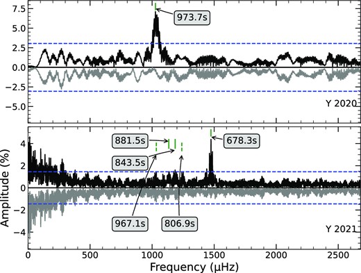
The LS periodogram of TMTS and SNOVA observations taken in 2020 and 2021, respectively. The horizontal dashed lines (in blue) denote the 4.0σ significance threshold. The upside-down grey curves represent the residuals of power spectra with significant frequencies being pre-whitened.
3.2 Input physics and model calculations
The latest version of the White Dwarf Evolution Code (wdec v16, Bischoff-Kim 2018) is used in this work to evolve grids for DAV models. This code includes the oxygen (O) profile in the core, parametrized by six parameters (i.e. h1–3, w1–3). This feature provides more accurate fitting results than previous version without it. The equation of state and opacity tables from the Modules for Experiments in Stellar Astrophysics (MESA; Paxton et al. 2011) are adopted in the current version of wdec. The standard mixing length theory (Bohm & Cassinelli 1971) and the mixing length parameter of 0.6 (Bergeron et al. 1995a) are adopted in the analysis. The explored parameter spaces of evolved WD models are shown in Table 3. For the initial ranges and crude steps in this table, 7558 272 WD models have been evolved. The model adopted here differs from those derived by considering the complete evolution. First, this model only considers the cooling phase of WD stars, while fully evolutionary models take into account the complete evolution of the progenitor stars and the WD cooling phases. Secondly, this model here is a large sample model grids including parametrized central core, while fully evolutionary models are typically not used for large sample model fitting. More details regarding the core parameters can be found in fig. 1 of Bischoff-Kim (2018) and the user manual (Bischoff-Kim & Montgomery 2018). In the fitting process, fine steps are used to optimize the fitting models.
The explored parameter spaces of WDs evolved by wdec.
| Parameters | Initial ranges | Crude steps | Fine steps | Optimal valuesa | Optimal valuesb |
|---|---|---|---|---|---|
| M*/M⊙ | [0.500, 0.850] | 0.010 | 0.005 | 0.760 ± 0.005 | 0.690 ± 0.005 |
| Teff(K) | [10 600, 12 600] | 250 | 10 | 12110 ± 10 | 12370 ± 10 |
| log(Menv/M*) | [1.50, 2.00, 3.00] | 0.50/1.00 | 0.01 | 2.00 ± 0.02 | 3.00 ± 0.01 |
| log(MHe/M*) | [2.00, 5.00] | 1.00 | 0.01 | 5.01 ± 0.04 | 4.99 ± 0.01 |
| log(MH/M*) | [4.00, 10.00] | 1.00 | 0.01 | 9.98 ± 0.02 | 7.00 ± 0.01 |
| XHe in mixed C/He/H region | [0.10, 0.90] | 0.16 | 0.01 | 0.25 ± 0.01 | 0.56 ± 0.01 |
| XO in the core | |||||
| h1 | [0.60, 0.75] | 0.03 | 0.01 | 0.73 ± 0.01 | 0.66 ± 0.01 |
| h2 | [0.65, 0.71] | 0.03 | 0.01 | 0.66 ± 0.01 | 0.71 ± 0.01 |
| h3 | 0.85 | – | 0.01 | 0.81 ± 0.03 | 0.85 ± 0.01 |
| w1 | [0.32, 0.38] | 0.03 | 0.01 | 0.35 ± 0.01 | 0.37 ± 0.01 |
| w2 | [0.42, 0.48] | 0.03 | 0.01 | 0.45 ± 0.01 | 0.46 ± 0.01 |
| w3 | 0.09 | – | 0.01 | 0.09 ± 0.01 | 0.12 ± 0.01 |
Notes. M* denotes the stellar mass, while Menv is the envelop mass. MH is the mass of hydrogen atmosphere, and MHe is the mass of He layer. XHe is the He abundance in the mixed C/He/H region, and XO is the O abundance in the core. The parameter h1 refers to the O abundance in the core centre, while w1 is the mass fraction of XO = h1. Parameters h2 and h3 are O abundance of two knee points on the reducing O profile. The w2 and w3 refer to the masses of the gradient regions of O profile.
Adopted solution.
Additional solution found by freeing the value of l.
3.3 The model fittings
For the model fittings, a root-mean-square residual σRMS is adopted in this work for the evaluation of fitting results.
In equation (1) above, n is the number of fitted observed modes, i.e. 6 for J2345. Pobs and Pcal are the observed periods and model calculated periods, respectively. During model fittings, only two digits behind decimal points of observed periods are used. Owing to the fact that periods 973.73 and 967.11 s are close and the amplitude of period 973.73 s is large, we assume that the period of 967.11 s is l = 2 mode, and the other five periods belong to the l = 1 mode. Additional analysis has been checked as well, leaving free the value of l for all periods. For the initial fitting, the combinations of parameter space ranges and crude steps are used to build the DAV models. This includes 7558 272 models, which are adopted to fit the observed six modes. The crude steps are chosen by considering the computational requirement for models. It takes around 12 s to evolve one model. Then, the parameter steps of models are narrowed down to fine steps around models with minimum σRMS. For the fine steps, there are three to five grid points for each parameter. For fine steps of mass, 0.005 is chosen because it is the same step size adopted in wdec. For the other fine steps, they are all chosen to be much smaller than their crude steps. In Table 3, there are six global parameters and six XO parameters. In order to find the minimum fitting error, the XO parameters are first fixed, and a grid of global parameters is generated. Then, the global parameters are fixed, and a grid of XO parameters is generated. The chosen fitting model will be nearly convergent to an optimal fitting model after repeating these two processes for a dozen times. Finally, the optimal model is obtained when σRMS = 0.21 s (the derived distance is calculated later as 98 pc). For the additional analysis, the optimal model is found when σRMS = 0.046 s and its derived distance is 103 pc. The optimal model parameters of adopted and additional solutions are listed in the fifth and last columns of Table 3, respectively. Although the optimal solution in additional analysis is achieved with a smaller fitting error of 0.046 s, the solution with a fitting error of 0.21 s is adopted, due to the latter solution results in only one l = 2 mode. With more high-degree modes in the adopted solution (more modes exist in the solution model as well), smaller fitting errors can be achieved, but it is not a reasonable choice comparing to the one with less high-degree modes. In addition, in order to explore models with thicker H and He envelops [−log(MHe/M*) = 2 and −log(MH/M*) = 4, which we did not include in the beginning due to limited computational power], a model grid containing 314 928 models is calculated. Independent model fittings are performed, yet the adopted solution listed in the fifth column of Table 3 is still preferred after comparison. On the other hand, in both solutions shown in Table 3, close periods 973.734 and 967.113 s are not both l = 1, meaning they are not likely to be components of a rotational triplet. The full width at half-height of the reciprocal of nσRMS is estimated as the error of each optimal value. It is known that modes with k ≫1 probe the most external part of the star. Thus, the lack of short-period modes in our observation reflected in larger errors in the core (h1–w3), compared to the errors estimated for L19-2 (Chen 2022). For L19-2, same models and approach have been applied, but its observations have detected more short-period modes, which yields much smaller errors in the core. According to the derived optimal values, J2345 is a relatively massive and hot DAV with a thin H atmosphere.
A colour graph of fitting error σRMS as functions of stellar mass and Teff is displayed in the left-hand panel of Fig. 4. The colour represents the fitting error σRMS as defined in equation (1). The grid consisting of stellar mass in the range of 0.500 and 0.850 M⊙ with a step of 0.005 M⊙ and Teff in the range of 10 600 and 12 600 K with a step of 10 K is included in the analysis, which contains 14 271 DAV models. All of other parameters are fixed to their optimal values in Table 3. The right-hand panel of Fig. 4 shows σRMS as functions of He-layer mass and envelope mass, which involves 7676 DAV models. The logarithm of envelope mass ranges from −2.00 to −3.00 with a step of 0.02, and the logarithm of He-layer mass ranges from −4.01 to −6.01 with a step of 0.02.
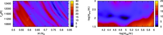
Left-hand panel: a colour graph of fitting error σRMS as functions of stellar mass and Teff. A total of 14 271 DAV stellar models are used in fit. Right-hand panel: a colour graph of fitting error σRMS as functions of He-layer mass and envelope mass. A total of 7676 DAV stellar models are used in the fit.
The sensitivity plots of eight parameters of the optimal model are shown in Fig. 5. Stellar mass, Teff, envelope mass, He-layer mass, H-atmosphere mass, He abundance in mixed C/He/H region, and h1 and w1 for the O profile versus fitting error σRMS are plotted in different subplots, respectively. Each panel of these parameters is plotted when all other parameters are fixed to the optimal values. The parameter values corresponding to the lowest σRMS indicate the optimal values. In Table 3, the mass of the shell of H ranges from |$10^{-10}\, M_{\ast }$| to |$10^{-5}\, M_{\ast }$|. However, our fitting is not limited to explore spaces in this range. Depending on the pre-optimal solutions of each iteration in the search for final optimal values of J2345, the initial ranges listed in Table 3 may be extended if pre-optimal value is near the range limit. For instance, it is shown in Fig. 5 that H masses less than |$10^{-10}\, M_{\ast }$| have been explored as well, since the optimal value is near the limit of initial lower range. Similar case can be found in the mass of the shell of He; spaces as low as |$10^{-6}\, M_{\ast }$| are explored as well, exceeding the lower limit of |$10^{-5}\, M_{\ast }$|. The core composition profiles and corresponding Brunt–Väisälä frequency for the optimal model are shown in Fig. 6, where the bumps are caused by composition gradient in different zones. There are some smaller bumps existing near horizontal axis 1 and 5 as well. After some simple investigations into this matter, we assume that those have something to do with wdec, rather than anything physical. One should note that these kinds of chemical profiles are in contrast with those derived from fully evolutionary computations. The existence of a C-buffer and several features in the chemical profile has been discussed extensively in De Gerónimo et al. (2019) for a DBV star.
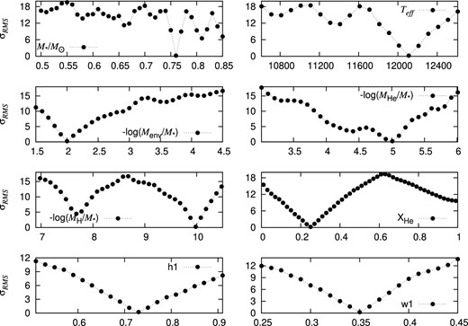
Sensitivity plots of eight parameters of the optimal model. Subplots are eight parameter values versus their root-mean-square residual σRMS.
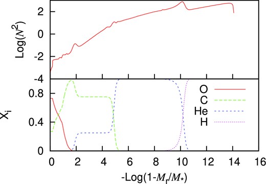
The core composition profiles and corresponding Brunt–Väisälä frequency for the optimal model. In the lower panel, the abundances of O, C, He, and H are plotted in red solid line, green dashed line, blue dashed line, and magenta dotted line, respectively. In the upper panel, the vertical axis is the logarithm of the square of buoyancy frequency. Three little bumps are present due to the existence of three element transition gradient zones.
In order to check the self-consistency of the best-fitting model, the distance derived from asteroseismology analysed results can be used to do an independent test. For the best-fitting model, the luminosity of J2345 is log(L/L⊙) = −2.685. The bolometric magnitude of the optimal model is Mbol = 11.45, using the correction Mbol = Mbol, ⊙ − 2.5 × log(L/L⊙) and assuming the bolometric magnitude of the Sun Mbol, ⊙ = 4.74 (Cox 2000). Since the bolometric correction (BC) in Gaia G band is not provided for J2345 in DR3, the BC in the V band is adopted. The BCs(V) for DA star model with Teff = 12 000 and 13 000 K are −0.611 and −0.828 mag, respectively, as listed in table 1 of Bergeron, Wesemael & Beauchamp (1995b). Therefore, for J2345 with Teff = 12 110 K, the linear interpolated BC(V) is −0.635 mag. The absolute V magnitude can be derived as MV = Mbol − BC(V) = 11.45 − (−0.635) = 12.085. By using the equation |$d=10^{(m_{V}-M_{V})/5+1}$|, the distance corresponding to the optimal model is 93 pc, given mV = 16.93 (Lasker et al. 2008). Comparing to the inverse parallax distance of 98 pc from Gaia DR3, there is ∼5 per cent error in the optimal model derived distance. Furthermore, the results corresponding to the optimal model are in agreement with the parameters obtained from spectral model fitting in Section 2.2. These two facts suggest that our asteroseismological results are self-consistent.
4 ROTATION PERIOD OF NEARBY M DWARF FROM TESS
J2345 was observed by TESS in sectors 17 and 24. They are both recorded in 120- and 1800-s exposures. Based on the LS (Scargle 1982) method, a noticeable period of ∼3.39 h is present in the power spectra of both TESS observations (Fig. 7), which is not detected in TMTS and SNOVA observations. Rebassa-Mansergas et al. (2019) listed J2345 and another star named Gaia DR2 1999127510436274048 as comoving stars (see table 1 in their paper), as they are located within about 3 arcsec and have similar parallaxes and proper motions from Gaia DR2. According to their SED fitting, the Teff values of these two stars are 11 750 and 2800 K, respectively, indicating that the comoving star is an M star. Since the image resolution of TESS is ∼21 arcsec per pixel and the brightness of M star is comparable to J2345 in TESS red band, the detected 3.39-h period may originate from the M star. First, the 3.39-h period is not plausible to be the pulsation period of J2345, as it is too long. Secondly, the power of 3.39-h period is much weaker in 2020 than in 2019 (see Fig. 7). Combining the fact that this period is not detected in 2021 observations from TMTS and SNOVA, it is most probable that this period is due to the rotation of the M star. The appearance and disappearance of a large dark spot can cause the variation observed in 2019 and 2020. The non-detection in 2021 further rules out the possibility that this period is due to eclipsing of a hidden companion, since the significance of orbital period signal should be stable. To further validate our hypothesis, the folded light curve of TESS observation in 2019 is fed to PHOEBE for modelling.
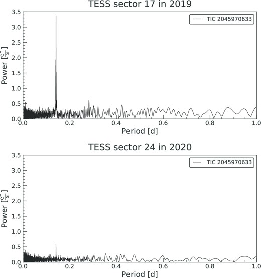
The LS periodogram of TESS 120-s observations taken in 2019 and 2020, respectively. The 3.39-h period becomes much weaker in 2020 than in 2019.
It is known that modelling stellar spots is difficult, as the observed light curve can be well fitted by one large spot or several smaller spots. Currently, PHOEBE does not have spot estimators for single stars. Therefore, we manually tuned the spot parameters to reproduce a similar light curve to mimic the phase-folded light curve of TESS in sector 17 (Fig. 8). The parameters of the star are set as Teff = 2800 K, mass = 0.21 M⊙, star radius = 0.15 R⊙, rotation period = 3.39 h, and inclination angle = 90°. The single large spot setting results in: an angular radius of 80°; the co-latitude of the centre of spot with respect to spin axis is 90°; longitude of the centre of the spot with respect to spin axis is 0°; and the relative temperature of the spot to the intrinsic temperature is 0.97. The direct image of this spot setting is shown in Fig. 9, corresponding to the model light curve at phase 0.75. It should be noted that this does not necessarily mean that this model setting is the real case. It is simply a demonstration to show that the TESS light curve in 2019 can be modelled by the rotation of a large dark spot on the M dwarf.
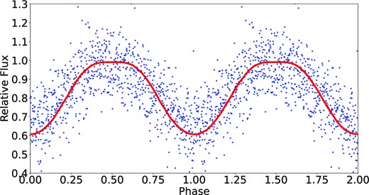
Phase-folded TESS light-curve modelling with PHOEBE. Blue dots are observed phase-folded TESS light curve in sector 17 with a 30-min exposure, while red line represents the PHOEBE reproduced light curve of a single star with a single large dark spot.
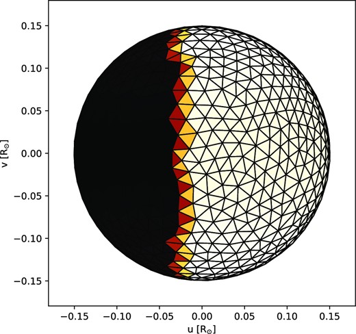
Mesh plot of PHOEBE model of a single star with a single spot, corresponding to the red line light curve at phase = 0.75 with an inclination angle of 90°. The star rotates from left to right.
5 DISCUSSION
According to the coordinates from Gaia DR3, the separation between J2345 and the M star is roughly 2.67 arcsec, corresponding to a projected separation of ∼15 au at 98 parsec away. Based on the parallaxes from Gaia DR3, the distances of the two stars in the line of sight are 94.6288 and 97.7039 parsec, respectively. Therefore, the actual separation should be at least 3 parsec, indicating that these two stars may be the result of a disrupted wide binary (Oh et al. 2017). There is no third star with similar proper motion at similar distance within 5 arcmin in Gaia DR3; thus, they do not belong to a large structure. The PanSTARRS images2 in z and y bands, which have the earliest and latest available images taken 1039 and 743 d apart, respectively, are checked as well. However, no obvious relative movements can be observed.
Given the newly released Gaia DR3, it is worth to check whether J2345 is a disc or halo WD, since halo WD is rare object of interest. The accurate measurements of J2345 include coordinates of RA = 356.2808 deg, Dec. = 58.2209 deg, parallax of 10.2350 mas, and proper motion of pmra = 28.9359 mas yr−1 and pmdec = 5.8859 mas yr−1. With the radial velocity of −67.7 ± 17.2 km s−1 derived from follow-up spectrum with WDTOOLS, the 3D heliocentric velocity U, V, and W of J2345 can be calculated following equations listed in Guo, Liu & Liu (2016). The probability calculated from U = −23.85 km s−1, V = −53.87 km s−1, and W = 9.88 km s−1 suggests that J2345 is likely a thick-disc star, not a halo WD (see Fig. 10). This result is consistent with the disrupted wide binary scenario, as wide binaries in the disc may be disrupted by passing stars, Galactic tides, and molecular clouds (Weinberg, Shapiro & Wasserman 1987; Jiang & Tremaine 2010). However, halo wide binaries are less likely to be disrupted by passing stars and molecular clouds since majority of their lifetime is spent outside the disc. Although some halo wide binaries will travel through the disc, the short duration due to their high spatial velocities makes it less probable to be disrupted (Weinberg et al. 1987).
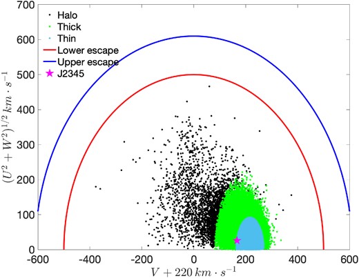
Gaia DR3-selected 1 kpc sample and J2345 plotted in the V + 220 km s−1 versus (U2 + W2)1/2 km s−1 plane. Halo, thick disc, and thin disc candidates are plotted in black, green, and light blue, respectively. Red and blue lines are lower and upper limits of the escape velocity of the Milky Way, respectively. Magenta star marks the location of J2345.
Since the asteroseismological analysis has provided the accurate mass of J2345, the rough evolution history of this WD can be learnt via stellar evolution models. First, the initial mass at ZAMS can be calculated as 3.08 M⊙, based on equation (2), which is derived from equation (5) in Cummings et al. (2018).
where Mi is the initial mass, while Mf is the final mass. This equation is a MIST-based semi-empirical initial–final mass relation. In table 1 of Renedo et al. (2010), for a WD star with Z = 0.01 and MWD = 0.767 M⊙, the lifetime of its main-sequence phase lasts for 0.232 Gyr. Thus, the main sequence plus cooling age of J2345 with M|$_{\mathrm{ WD}}=0.760\pm 0.005\, \mathrm{M}_{\odot }$| is TMS + Tcooling ≈ 200 + 700 = 900 Myr. This is less than 1 per cent of the lifetime of the companion M star with Teff = 2800 K, assuming they formed simultaneously.
On another note, if the initial mass of J2345 at ZAMS is 3.08 M⊙, it should be a B9- or A0-type star (Cox 2000). However, the companion of its progenitor is a late M-type star. Therefore, it is also possible that there was an accretion process, as binaries formed in the same region tend to have similar spectral types, and the WD mass in accreting system (i.e. mean MWD ∼ 0.8 M⊙ for CV) is usually higher than the average mass (∼0.6 M⊙) of single WD (Zorotovic & Schreiber 2020).
6 SUMMARY
In this work, a newly discovered ZZ ceti J2345 is reported and analysed. The discovery is the result of searching for variable WDs from the minute-cadence photometric survey TMTS. By cross-matching Gaia EDR3 WD catalogue with the TMTS catalogue, there are more than a thousand common WD candidates. Each is planned to be visually inspected for variation that can be attributed to WD pulsation, binary eclipsing, and planetesimal transiting. Many interesting sources have been identified, and this is the very first paper to report our findings in TMTS.
Based on two and five night observations of TMTS and SNOVA, there are six pulsating modes identified after pre-whitening. Those modes are used to perform the asteroseismological analysis. By adopting the latest version of wdec, there are 7558 272 WD models evolved for the parameter spaces listed in Table 3. To find the optimal model, parameter steps and spaces are slowly narrowed down repeatedly, in accordance of the fitting result. At last, the optimal model is found and its parameter values are listed in Table 3. To test our mode identification, additional analysis of freeing the values of l for all periods has been checked and compared. Based on the comparison and analysis in Section 3.3, we believe that our identification is a more reasonable choice. From the asteroseismological result, it can be learnt that J2345 is a massive and relatively hot pulsating WD with moderately thin H atmosphere. The final results are quite consistent with the parameters derived from spectral fitting of follow-up spectrum. In addition, the distance deduced from asteroseismological results is in agreement with the inverse parallax derived distance from Gaia DR3, implying a good self-consistency.
An evident period of ∼3.39 h is found to exist in two observations of TESS. Given the fact that the significance of this signal weakens considerably between two TESS observations, we propose that this period is attributed to the rotation of dark spot on a comoving M star. The TESS light curve taken in 2019 has been modelled by Phoebe with a single star plus one dark spot model. The result suggests that a synthetic light curve representing a very large dark spot, nearly covering half of the M dwarf’s surface, can be reproduced to mimic the observed TESS light curve. This implies that the identified period and light-curve evolution from the TESS data can be explained by stellar spot. However, the resulted parameters of the spot should be treated with caution, as the real case may be caused by several spots with different sizes and locations. With the newly released Gaia DR3, the 3D heliocentric velocity UVW of J2345 is calculated, and the result indicates that J2345 is likely a thick-disc star instead of a halo WD. Furthermore, since the initial progenitor mass of WD can be estimated from current mass, its whole evolution history can be learnt. By comparing to a well-studied WD with similar mass, we estimate the lifetime of the main-sequence phase of J2345 being as about 200 Myr and current age as 900 Myr plus cooling time.
ACKNOWLEDGEMENTS
The authors acknowledge the National Natural Science Foundation of China (NSFC) under grants 12203006, 12033003, 12288102, U1938113, 11773035, 12090044, 11833002, and 11633002. This work was also supported by the Ma Huateng Foundation, the Scholar Program of Beijing Academy of Science and Technology (DZ:BS202002), the Tencent Xplorer Prize, and CSST projects: CMS-CSST-2021-B03, the Innovation Project of Beijing Academy of Science and Technology (11000023T000002062763-23CB059 and 11000022T000000443055).
This work has made use of data from the European Space Agency (ESA) mission Gaia (https://www.cosmos.esa.int/gaia), processed by the Gaia Data Processing and Analysis Consortium (DPAC; https://www.cosmos.esa.int/web/gaia/dpac/consortium). Funding for the DPAC has been provided by national institutions, in particular the institutions participating in the Gaia Multilateral Agreement. This research has made use of the SIMBAD data base, operated at CDS, Strasbourg, France (Wenger et al. 2000).
DATA AVAILABILITY
The TESS data used in this article can be accessed via https://archive.stsci.edu/missions-and-data/tess. The TMTS and SNOVA photometric and 3-m spectral data can be obtained by contacting the corresponding authors.
Footnotes
Frequency Extraction for Lightcurve exploitation, which was developed by Stéphane Charpinet. See details of the code in (Charpinet et al. 2010).
