


ABSTRACT
Our ability to interpret observations of galaxies and trace their stellar, gas, and dust content over cosmic time critically relies on our understanding of how the dust abundance and properties vary with environment. Here, we compute the dust surface density across cosmic times to put novel constraints on simulations of the build-up of dust. We provide observational estimates of the dust surface density consistently measured through depletion methods across a wide range of environments, going from the Milky Way up to z = 5.5 galaxies. These conservative measurements provide complementary estimates to extinction-based observations. In addition, we introduce the dust surface density distribution function – in analogy with the cold gas column density distribution functions. We fit a power law of the form log f(ΣDust) = −1.92 × log ΣDust − 3.65, which proves slightly steeper than that for neutral gas and metal absorbers. This observed relation, which can be computed by simulations predicting resolved dust mass functions through 2D projection, provides new constraints on modern dust models.
1 INTRODUCTION
Dust grains absorb stellar light in the ultraviolet (UV)–optical wavelengths and re-emit it in the far-infrared, which represents 30–50 per cent of the radiative output of a galaxy (Roman-Duval et al. 2017). Therefore, our ability to interpret observations of galaxies and trace their stellar, gas, and dust content with redshift across the entire spectral range critically relies on measurements of the dust abundance and properties that vary with environment and cosmic times. This in turn requires us to understand the processes responsible for dust formation, destruction, and transport, as well as their associated time-scales.
A fraction of metals in the interstellar medium of galaxies in both the local and high-redshift Universe resides in microscopic solid particles or dust grains (Field 1974; Savage & Sembach 1996; Jenkins 2009a; De Cia et al. 2016). Interstellar dust has manifold impact on the physics and chemistry of the interstellar medium (Zhukovska et al. 2016; Zhukovska, Henning & Dobbs 2018; Galliano 2022) as well as the intracluster medium (Shchekinov, Nath & Vasiliev 2022). Because dust locks some elements away from the gas phase, it affects our measurements of the metallicity of galaxies. One of the most important roles of interstellar grains is that they facilitate the formation of molecular hydrogen, H2, on their surfaces (Hollenbach & Salpeter 1971). The H2 molecule is the main component of molecular clouds, which are the cradle of star formation in most of the Universe (Klessen & Glover 2016). Because dust absorbs UV emission from young massive stars and re-emits it in the infrared, the spectral energy distribution from dust is one of the primary indicators of star formation (Calzetti et al. 2000).
Yet, in both local and high-redshift galaxies, the dust production rates in evolved stars (Bladh & Höfner 2012; Riebel et al. 2012) and supernova remnants (Matsuura et al. 2011; Leśniewska & Michałowski 2019; Slavin et al. 2020) are largely insufficient compared to the dust destruction rates in interstellar shocks (Jones, Tielens & Hollenbach 1996) to explain the dust masses of galaxies over cosmic times (Morgan & Edmunds 2003; Boyer et al. 2012; Zhukovska & Henning 2013; Rowlands et al. 2014). This so-called dust budget crisis poses an important challenge to our modelling of dust into a cosmological context (Mattsson 2021).
Observationally, the amount of dust in astrophysical objects has been quantified with a number of different methods probing various dust signatures. Extinction refers to the amount of light dimming due to all the material lying along the line of sight between the astrophysical object and the observer. Extinction is therefore an integrated quantity that encapsulates absorption and scattering away from the line of sight. The observational determination of extinction requires backlights such as stars, gamma-ray bursts, quasars, or other objects with much smaller angular extent than a galaxy. The extinction at a given wavelength results from a combination of the grain size distribution (Mattsson 2020), metallicity (Shivaei et al. 2020a), and the optical properties of the grains (which is itself dependent on the chemical composition of the grains). Therefore, the extinction scales with dust column density or surface density. Similarly, infrared emission has been used to probe the dust content of galaxies (Chiang et al. 2021). In particular, significant work has been done for characterizing these quantities in galaxies beyond the Milky Way, assessing observational constraints on both the integrated values (e.g. Rémy-Ruyer et al. 2014; De Vis et al. 2019) and spatially resolved values within galaxies (e.g. Vílchez et al. 2019). These works have placed particular emphasis on the variation of the dust properties with metallicity, stellar mass, star formation rate, and gas content of the galactic environments, as these help shape our understanding of the factors that drive the formation/destruction balance of dust. Reddening, expressed through the colour excess, E(B − V), quantifies the differential extinction.
Attenuation represents the effect of dust on the light continuum from the geometric mix of stars and dust in galaxies. It thus reflects the net effect on light due to a combination of multiple effects, including extinction, scattering back into the line of sight and contribution from unobscured stars (Salim & Narayanan 2020). Reddening is often expressed in terms of UV continuum slope, β (Shivaei et al. 2020b). The UV continuum slope depends on the column density of dust along the line of sight to the observer that is dimming the UV light of background objects. A fully consistent comparison between depletion-estimated extinction and colour-based estimates is found in Konstantopoulou et al. (2023).
The total far-infrared emission is a proxy for the total dust mass. At z > 5, that emission is successfully probed at mm wavelengths with facilities such as Atacama Large Millimeter Array (ALMA). The dust temperature, however, is less well constrained in these early times (see fig. 1 of Bouwens et al. 2020), leading to a degeneracy in the current estimates (Faisst et al. 2020; Sommovigo et al. 2020, 2022; Bakx et al. 2021; Drew & Casey 2022; Ferrara et al. 2022; Fudamoto et al. 2022; Viero et al. 2022; Chen et al. 2022a). Alternatively, the dust mass is being derived from the mm continuum of high-redshift galaxies and the gas mass is then estimated assuming a dust-to-gas ratio – often taken to be the value of the Milky Way (Scoville et al. 2017; Dunne et al. 2022, but see Popping & Péroux 2022). The ratio of dust emission in infrared to the observed UV emission, known as the infrared excess (IRX), is a measure of the UV dust attenuation. The attenuation/extinction curve/law is characterized by its slope and normalization (e.g. Calzetti et al. 2000). Two galaxies having the same attenuation curves (i.e. same shape) might still differ in their normalization (i.e. column density of dust). The two quantities, β and IRX, are often related into one diagram (Meurer, Heckman & Calzetti 1999; Faisst et al. 2017; Shivaei et al. 2020b). The relation is sensitive to a range of interstellar properties, including dust geometries, dust-to-gas ratios, dust grain properties, and the spatial distribution of dust. The relation provides a powerful empirical constraint on dust physical properties because it laid the foundation for a straightforward correction of UV emission in galaxies where infrared observations are lacking (especially at higher redshifts), based on the easily observable UV slope (or colour).
Dust is made of some of the available metals produce by stars. In the interstellar medium, a fraction of these elements is in the gas, and the rest is locked up in dust. Indeed, most metals are underabundant in the interstellar gas of the Milky Way (Jenkins 2009a), reflecting the amount of dust in our galaxy. Dust depletion can be used to give hints on the dust composition (Savage & Sembach 1996; Jenkins 2014; Dwek 2016; Mattsson et al. 2019; Roman-Duval et al. 2022a) and this often indicates that significant amounts of Fe-rich dust should be present in the interstellar medium. Dust measurements based on depletion estimated at UV and optical wavelengths might suffer from a bias where the dustier systems would be obscured at these wavelengths. In that sense, dust depletion provides conservative measurements that can be seen as a lower limit on the total amount of dust in a population. Depletion measurements provide a direct estimate of the dust content (Dwek 1998; Draine & Li 2007; Galliano, Galametz & Jones 2018). The depletion can be used to calculate the extinction through the gas which is proportional to the column density of metals (see equation 1 of Savaglio, Fall & Fiore 2003). In their fig. 9, Wiseman et al. (2017) offer a comparison of the two measurements between depletion-estimated extinction and colour-based estimates in a sample of Gamma-Ray Bursts, indicating significant discrepancies highlighting the possible limitations described above (see also De Cia et al. 2013; Zafar et al. 2014).
These multiple observational results have triggered a number of simulation efforts. These works come into two main families: (i) semi-analytical models that use empirical relation to approximate some of the physical processes at play and (ii) hydrodynamical cosmological simulations that include full treatments of dust production and destruction. Contemporary models have reached a new level of realism by including a large number of physical processes (Draine 2003). Dust shattering refers to the breaking of large grains into small dust grains, due to high-velocity collisions. Conversely, coagulation describes the processes of large grains being made out of smaller entities because of low-velocity collisions. Therefore, both these processes do not change the mass but the size distribution of dust grains. Sputtering refers to dust destruction by shocks, including those produced by Supernovae blasts. Astration reflects the process of dust being absorbed by stars. We note that the same processes can both produce and destroy small/big grains, so that the production sources and destruction sinks are complex processes to simulate.
A number of efforts based on semi-analytical models have made predictions on the dust mass of galaxies (Bekki 2015; Pantoni et al. 2019; Gjergo et al. 2020; Lapi et al. 2020; Dayal et al. 2022) and associated dust mass function (Popping, Somerville & Galametz 2017; Vijayan et al. 2019; Triani et al. 2020). As subset of these studies has provided information on the dust surface density specifically (Bekki 2013, ; Gjergo et al. 2020; Osman, Bekki & Cortese 2020). In parallel, there have been a number of works introducing dust physical processes within hydrodynamical cosmological models (Moseley, Teyssier & Draine 2023). Many report estimates of the dust mass density (Gioannini et al. 2017; Aoyama et al. 2018; Lewis et al. 2022), while others report the dust mass function (McKinnon et al. 2017; Graziani et al. 2019; Hou et al. 2019; Li, Narayanan & Davé 2019; Baes et al. 2020). A number of these efforts have made predictions on dust surface densities in particular, as the ones presented here (McKinnon, Torrey & Vogelsberger 2016; Trayford & Schaye 2019).
The goal of this work is two-fold. On one hand, we provide observational estimates of the dust surface density consistently measured through depletion methods across a wide range of environments, going from the Milky Way up to z = 5.5 galaxies. While previous works have estimated the dust mass in local galaxies (De Vis et al. 2019; Casasola et al. 2020; De Looze et al. 2020; Millard et al. 2020; Morselli et al. 2020; Nanni et al. 2020; Galliano et al. 2021), this study focuses on the dust column density. On the other hand, we introduce the dust surface density distribution function – in analogy with the gas [N(H i) or N(H2)] column density distribution functions (Péroux et al. 2003; Zwaan et al. 2005; Zwaan & Prochaska 2006; Klitsch et al. 2019; Péroux & Howk 2020; Szakacs et al. 2022). Spatially resolved simulations predicting the dust-mass function (Millard et al. 2020; Pozzi et al. 2020) can predict the dust surface density distribution function through 2D projection. Thus, the observed dust surface density distribution function potentially offers new constraints on modern dust models.
The manuscript is organized as follows: Section 2 presents the methods used in this study. Section 3 details how dust surface density relates to the global physical properties of galaxies. We summarize and conclude in Section 4. Here, we adopt an H0 = 67.74 km s−1 Mpc−1, ΩM = 0.3089, and ΩΛ = 0.6911 cosmology. We use the latest solar abundance values from Asplund, Amarsi & Grevesse (2021).
2 DIFFERENTIAL DUST DEPLETION
2.1 Dust depletion in our Galaxy
2.1.1 Methodology
The depletion of metals is differential, with some elements showing a higher affinity for incorporation into solid-phase grains than others, based on their chemical properties (Pettini et al. 1997; Vladilo 2002; Jenkins 2009a). The differential nature of elemental depletion has traditionally been used to correct the observed abundance for unseen metals. Early works used lightly depleted elements to derive abundances (e.g. focusing on Zn or S or to a lesser degree Si). More recent works have taken advantage of the patterns of differential depletion to estimate the extent of the dust-depletion correction. These efforts follow the spirit of Vladilo (1998) and Jenkins (2009a), using the observed abundances to study the dust depletion beyond the Milky Way (Jenkins & Wallerstein 2017; Roman-Duval et al. 2022a).
Specifically, De Cia et al. (2016) developed a method to characterize dust depletion, δX, without assumption on the total gas + dust metallicity. This is achieved through the study of relative abundances of several metals with different nucleosynthetic and refractory properties, as follows. The relative gas-phase abundance of the metals X and Y is written: |$[\mathrm{ X}/\mathrm{ Y}] = \rm log (N(\mathrm{ X})/N(\mathrm{ Y}))-log(N(\mathrm{ X})_{\odot }/N(\mathrm{ Y})_{\odot })$|. This approach enables to calculate the depletion without assumptions on the total metallicity of the gas, including metals locked on to dust grains (see also De Cia 2018a; De Cia et al. 2021). We derive the depletions of different elements as follows:
where [Zn/Fe]fit traces the overall amount of dust depletion and is taken from De Cia et al. (2021). This quantity is equivalent to the observed [Zn/Fe], although it is based on the observations of all available metals. The coefficients A2X and B2X are taken from Konstantopoulou et al. (2022).
The total dust-corrected metallicity is then computed as
where [X/H]total is the total metallicity including metals locked into dust grains, [X/H]observed is the observed abundance of X in the gas phase, and δX, i.e. the logarithm of the fraction of X in the gas phase. Given that each element has a different propensity to deplete onto dust grains, the observations of multiple element ratios provide a measure of the interstellar depletions for various elements X. Given estimates of δX and observations of [X/H]observed, one can derive the quantity: [X/H]total.
2.1.2 Observational results in the Milky Way
In the Milky Way, depletions have been studied for many heavy elements in several hundreds of sightlines through the diffuse neutral medium (Field 1974; Phillips, Gondhalekar & Pettini 1982; Jenkins 2009b; De Cia et al. 2021). Here, we make use of results from two works: while Jenkins (2009a) assumes solar metallicity (and solar abundance pattern) for the Milky Way, De Cia et al. (2021) report both depletion and metallicity measurements along different line of sight. For consistency with other measurements and to avoid complications related to ionization corrections, we focus here on log N(H) ≥ 20.3 measurements from Jenkins (2009a). We also note that the methodology of Jenkins (2009a) follows the one presented for the Magellanic Clouds next as a fixed global metallicity is assumed. These studies indicate that in total about 50 per cent of the metals in the Milky Way’s interstellar medium are incorporated into grains (Draine 2003). The dust-to-gas (DTG) and dust-to-metal (DTM) mass ratios are calculated from these values of the dust depletions (see Section 3).
2.2 Dust depletion in the Magellanic Clouds
2.2.1 Methodology
The method that we use to estimate the amount of dust in the Magellanic Clouds is slightly different from the one used to estimate the same quantity in the Milky Way. The depletion for element X is expressed as follows:
where |$[\mathrm{ X}/\mathrm{ H}]_{\rm assumed\_total} = \log (\mathrm{ X}/\mathrm{ H})_{\rm assumed\_total}-\log (\mathrm{ X}/\mathrm{ H})_{\odot },$| is the total abundance of element X (gas + dust) that here is assumed to be equal to the abundance of element X in the photospheres of young stars that have formed out of the interstellar medium (as done for the Milky Way by Savage & Sembach 1996; Jenkins 2009a; Tchernyshyov et al. 2015; Jenkins & Wallerstein 2017; Roman-Duval et al. 2019). These works compare the chemical abundances in neutral interstellar gas based on UV spectroscopy to stellar abundances of OB stars and H ii regions (e.g. Luck et al. 1998; Hunter et al. 2007; Trundle et al. 2007; Toribio San Cipriano et al. 2017) to estimate δX from equation (3). In principle, there could be variations of the metallicity of the neutral interstellar medium in the Magellanic Clouds. We stress that the approach described in this section is therefore different from the ones reported in other sections for the Milky Way and for high-redshift galaxies.
2.2.2 Observational results in the Large Magellanic Cloud
The Large Magellanic Cloud lies just 50 kpc from us (Subramanian & Subramaniam 2009). Its dust content is probed through its extinction map (Furuta et al. 2022), while dust reddening (Chen et al. 2022b) and extinction (Gordon et al. 2003) have been measured in both the Large and Small Magellanic Clouds as well as dust emission (Chastenet et al. 2017). Recently, the Large Magellanic Cloud has been the focus of an HST Large Program dubbed ‘The Metal Evolution, Transport, and Abundance in the Large Magellanic Cloud’ (METAL) and introduced in Roman-Duval et al. (2019, 2021) demonstrates that the depletion of different elements in these data are tightly correlated with the gas (hydrogen) surface density. Roman-Duval et al. (2022a) further make a new appraisal of the dust estimates in the Milky Way, Large and Small Magellanic Clouds. The Galaxy is more strongly affected by dust depletion than the Large Magellanic Cloud, and even more than the Small Magellanic Cloud. Nevertheless, the way different elements deplete into dust is very similar between these various environments (De Cia 2018a; Konstantopoulou et al. 2022). Here, we use the data shown in fig. 7 of Roman-Duval et al. (2022a), which also include results from Tchernyshyov et al. (2015). We use a constant metallicity throughout the cloud, taken to be [X/H] = −0.30 (Roman-Duval et al. 2022a).
2.2.3 Observational results in the Small Magellanic Cloud
Similarly, depletion of gas-phase metal abundances are clearly seen in the Small Magellanic Cloud, situated at about 60 kpc (Subramanian & Subramaniam 2009), though with a smaller degree of depletion reflecting the lower dust-to-metal mass ratio in this system. Initial works from Tchernyshyov et al. (2015) and Jenkins & Wallerstein (2017) provide the first estimates of dust depletion in multiple lines of sight. Here, we use the observations displayed in fig. 6 of Roman-Duval et al. (2022a). These works assume a constant metallicity throughout the Small Magellanic Cloud, taken to be [X/H] = −0.70 (Roman-Duval et al. 2022a).
2.3 Dust in high-redshift Galaxies
2.3.1 Methodology
Given the presence of dust in a broad range of galaxies, depletion is naturally expected to be also detected in the material traced by high-redshift absorption lines seen against the background light of bright sources. In extragalactic systems, there have been numerous studies of diffuse neutral medium depletions, facilitated by the redshifting of the rest-frame UV absorption lines in the visible range (Ledoux, Bergeron & Petitjean 2002; Vladilo 2002; De Cia et al. 2016; Bolmer et al. 2019a). Similar to the Milky Way, we derive the dust-to-gas ratios for individual absorption systems from the elemental depletions. Because the behaviour of each metal species varies (Jenkins 2009a), the estimates of the depletion, δX, for each individual element, X, are derived from the dust sequences following the approach highlighted by De Cia et al. (2016, 2018) and Péroux & Howk (2020). The methodology used here is therefore identical to the one described in Section 2.1.1.
2.3.2 Observational results in gamma-ray burst hosts
Gamma-ray burst events in particular probe the insterstellar medium of their galaxy hosts. These systems have been used to probe the dust and metals in gamma-ray burst host galaxies (Savaglio & Fall 2004; Schady et al. 2007; De Cia et al. 2012; Zafar & Møller 2019). Here, we report observations from Bolmer et al. (2019a), which offer a set of dust-depletion estimates based on the correction from De Cia et al. (2016), hydrogen column density and metallicity for a sample of gamma-ray bursts.
2.3.3 Observational results in quasar absorbers
Quasar absorbers probe the gas inside and around hundreds of foreground galaxies unrelated to the background quasars (Pettini et al. 1994; Dessauges-Zavadsky et al. 2004; Rafelski et al. 2012). There is strong evidence for the differential depletion of metals in the quasar absorbers observed both for the neutral gas (De Cia et al. 2016, 2018; Péroux & Howk 2020) as well as for partially ionized gas (Fumagalli, O’Meara & Prochaska 2016; Quiret et al. 2016). The depletion in quasar absorbers is typically smaller than in the Milky Way (De Cia et al. 2016; Konstantopoulou et al. 2022; Roman-Duval et al. 2022b; Konstantopoulou et al. 2023). In addition, the abundance ratios change in a similar way from local to high-redshift galaxies (De Cia 2018b; Konstantopoulou et al. 2022), indicating that the depletion of dust evolves homogeneously all the way to high-redshift systems. These results also imply that grain growth in the interstellar medium is an important process of dust production
Here, we use the values of dust depletion summarized by Péroux & Howk (2020), which are based on results from De Cia et al. (2018) with some additional updates (see footnote 5 of Péroux & Howk 2020). We note that only a small fraction (of the order of 10 per cent) of these systems have detections of molecular hydrogen, N(H2). In addition, when detected, the fraction of molecular gas in the cold phase is also found to be small (∼0.01 per cent, see Petitjean et al. 2000; Noterdaeme et al. 2008; Balashev et al. 2019). For these reasons, we neglect the molecular hydrogen gas in quasar absorbers and assume N(H) = [N(H i)].
3 OBSERVED DUST SURFACE DENSITY
3.1 Methodology
The characterization of the bulk statistical properties of dust involve assessing the dust-to-gas (DTG) and dust-to-metal (DTM) mass ratios. The former is the fraction of the interstellar mass locked into dust grains; the latter is the fraction of the metal mass incorporated into the solid phase. The dust-to-gas ratio for an individual element, X, is related to its depletion, δX, and its dust-to-metal ratio as follows:
where Z|$_{\rm total}^{\rm X}$| is the intrinsic abundance of X expressed by mass (e.g. Vladilo 2004; De Cia et al. 2016). We derive the δX from the differential depletion of various elements as described in Section 2, and use them to calculate the individual DTGX (equation 5).
To obtain a global DTM ratio expressed for all the elements and in mass fraction, we then average the DTMX and weight them by elemental abundances and atomic weight for the Milky Way and the Magellanic Clouds (as also done in Roman-Duval et al. 2021). For the high-redshift galaxies, we derive the global DTM from the DTG as follows:
For this calculation, we include the 18 elements which depletion have been characterized by Konstantopoulou et al. (2022), though C, O, Si, Mg, and Fe contribute a major fraction of the total dust mass (see also Konstantopoulou et al. 2023). In the calculation, we also include all the volatile metals that have an element abundance higher than 12 + log(X/H) >3 (table 1 of Asplund et al. 2009, see also Asplund et al. 2021), most notably the N and Ne, which do not contribute to the dust budget, but contribute to the metal budget.
We then directly calculate the dust surface density that provides a observationally based measurements of the dust quantity. Specifically, we use several UV-based depletion measurements to calculate the dust mass surface density, ΣDust, in various environments. To this end, we couple observations of the total dust-to-gas ratio, DTG, described above with estimates of the column density of hydrogen gas, both in its atomic and molecular phases. We derive the dust surface densities as
where the total hydrogen column density is N(H) = N(H i) + 2N(H2), the sum of N(H i) and two atoms of hydrogen, N(H2), expressed in atoms cm−2. The quantity ΣGas is the gas surface density, mH is the hydrogen mass mH = 1.67 × 10⁻²⁴ g, and μ is the mean molecular weight of the gas which is taken to be 1.3 (76 per cent hydrogen and 24 per cent helium by mass). The dust surface density, ΣDust, is therefore expressed in g cm−2 or alternatively in M⊙ kpc−2. The resulting values for each of the systems are listed in the table available online, an excerpt of which is presented in the Appendix A.
3.2 Dust surface density as a function of gas properties
For completeness, we start by briefly summarizing the relations between the dust surface densities and galaxy physical properties. This work intentionally refrains to plot dust-to-gas ratio relation with galaxy’s properties since those have presented elsewhere (e.g. Popping & Péroux 2022). Fig. 1 displays the dust surface density as a function of cosmic time. In this figure and the followings, the left y-axis displays the dust surface density in units of g cm−2 and the right y-axis in units of M⊙ kpc−2. We stress that all these dust surface densities are derived from depletion measurements performed in absorption at UV wavelengths. The shade of colours from light to dark refers to the Milky Way, the Large and Small Magellanic Clouds, gamma-ray bursts, and quasar absorbers at z > 0. There is a clear trend of increasing dust surface density with cosmic time with a large scatter at any given redshift, as expected from the build up of metals and associated dust with time. Gamma-ray burst host galaxies overall have higher dust surface densities than quasar absorbers at the same redshift. This is consistent with gamma-ray bursts exploding in inner regions of their host galaxies, while quasar absorbers probe peripheral regions of the intervening galaxies where the sky cross-section is the largest (Prochaska et al. 2007; Fynbo et al. 2008).
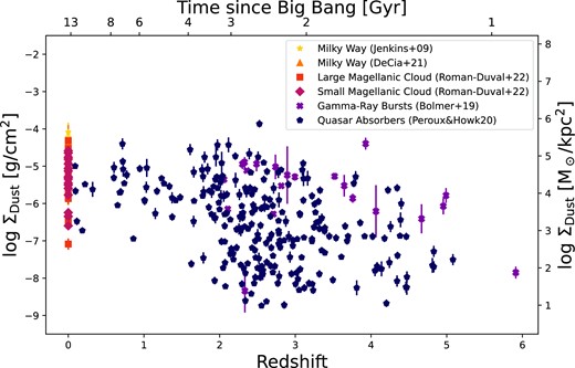
Dust surface density as a function of cosmic times. In this figure and the following, the dust column densities are derived from depletion measurements performed in absorption at UV wavelengths. The shade of colours from light to dark refers to the Milky Way, the Large and Small Magellanic Clouds, gamma-ray bursts, and quasar absorbers at z > 0. We note that gamma-ray burst galaxy hosts preferentially lie above the quasar absorbers. There is also a clear trend of increasing dust surface density with cosmic time with a large scatter at any given redshift, as expected from the building of dust with time.
Fig. 2 shows the dust surface density as a function of cold gas surface density. The cold gas refers to the sum of neutral atomic, H i, and molecular, N(H2), except for quasar absorbers where the molecular gas is found to be negligible (Ledoux, Petitjean & Srianand 2003). The grey lines show constant dust-to-gas ratios in steps of 1 dex. The dust column densities roughly follow the total hydrogen column densities, though with a 4-order of magnitude spread at a given ΣGas. Roman-Duval et al. (2014) used resolved Herschel infrared maps of Magellanic clouds in combination with 21 cm, CO, and H α observations to infer the relation between the atomic, molecular, and ionized gas with dust surface density. The authors report a clear trend of increasing dust surface density with increasing gas surface density in the diffuse interstellar medium, albeit for a medium with consistent metallicity. Our depletion-derived results show a similar scaling in Fig. 2. Roman-Duval et al. (2017) further explore the relation based on IRAS and Planck observations and find an increase by a factor three of the dust-to-gas ratio going from the diffuse to the dense insterstellar medium, in line with elemental depletions results. In the Milky Way (Jenkins 2009a) and Small Magellanic Cloud (Jenkins & Wallerstein 2017), the fraction of metals in the gas phase decreases with increasing hydrogen volume density and column density, albeit at different rates for different elements. Gamma-ray burst host galaxies display low dust surface densities in comparison with quasar absorbers while still bearing large amounts of gas (Jakobsson et al. 2006; Fynbo et al. 2009), even at relatively high gas surface densities. One possible reason for this difference is that Gamma-Ray Burst host galaxies have overall low metallicities and low dust content (Savaglio, Glazebrook & Le Borgne 2009; Krühler et al. 2015; Perley et al. 2016), although dustier systems do exist (Perley et al. 2011, 2013). We cannot exclude that systems with high dust surface density (even in the low-metallicity surface density regime) are missing from current sample based on UV dust-depletion observations. Interestingly, there is a dearth of systems with high gas surface density and low dust surface density which cannot be attributed to an observational bias, because systems lying in this parameter space – if they exist – would have small extinction.
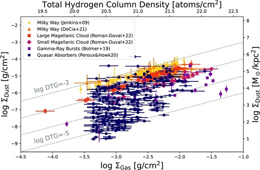
Dust surface density as a function of cold gas surface density. The grey lines represent constant dust-to-gas ratios in steps of 1 dex. The cold gas refers to the sum of neutral atomic, H i, and molecular, N(H2), except for quasar absorbers where the molecular gas is found to be negligible (Ledoux et al. 2003). Overall, the dust column densities follow the total hydrogen column densities with a 4-order of magnitude scatter.
The top panel of Fig. 3 displays the dust surface density as a function of gas metallicity. There is a relatively tight correlation between the dust column densities and the dust-corrected metallicity estimates at all cosmic times. Works from Jenkins (2009a); Roman-Duval et al. (2022b) report dust-depletion measurements assuming a global metallicity of [X/H] = 0 for the Milky Way, [X/H] = −0.30 for the Large Magellanic Cloud and [X/H] = −0.70 for the Small Magellanic Cloud. Additionally, the top panel of Fig. 3 shows a clear correlation between Σdust and metallicity. These results are in line with the dust-to-metal ratio increasing with metallicity (De Cia et al. 2013; Wiseman et al. 2017; Péroux & Howk 2020). The bottom panels of Fig. 3 illustrate the distribution in dust surface density at fixed metallicity materialized by the grey shaded areas in the top panel. In the Large Magellanic Clouds in particular, the dispersion in Σdust is larger than in quasar absorbers for a given metallicity, providing further evidence that the metallicity within the Clouds might vary. Likewise, we note that the Magellanic Clouds dust distributions are skewed towards higher values than quasar absorbers with the similar metallicity. This effect might be related to (i) quasar absorbers probing random position in the galaxy, and therefore being more likely to probe the outermost parts, and (ii) Magellanic Clouds are infalling satellites, so the gas compression coming from the ram pressure might boost dust formation by increasing the densities. We stress that further differences in Σdust might be not revealed here because of the assumption of fixed metallicity in the Magellanic Clouds.
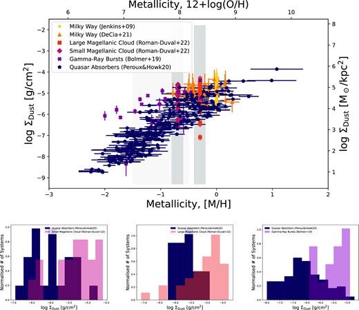
Top panel: Dust surface density as a function of gas metallicity. There is also a tight correlation between the dust surface densities and the dust-corrected metallicity estimates at all cosmic times. For a given metallicity, quasar absorbers have lower surface density of dust than gamma-ray burst host galaxies and the Milky Way, which are closer to the denser and colder parts of their galaxies. The Milky Way values from Jenkins (2009a) and the Large & Small Magellanic Clouds (Roman-Duval et al. 2022a) are assumed to have one global metallicity each. Bottom panels: Distribution of dust surface density in quasar absorbers, the Magellanic Clouds, and gamma-ray bursts at fixed metallicity. The bottom left panel displays observations for the Small Magellanic Cloud, the bottom middle panel shows data for the Large Magellanic Cloud, while the bottom right represents measurements for gamma-ray bursts. At fixed metallicity, the distribution in dust surface density in the Large Magellanic Cloud is wider than that for quasar absorbers. Similarly, at a given metallicity, Σdust is higher in gamma-ray bursts that are likely closer to the denser and colder parts of their galaxies than quasar absorbers.
The right most panel of Fig. 3 shows a comparison of quasar absorbers with gamma-ray bursts in the range −1.5 < [M/H] < −0.5 indicating that the latter have larger dust surface density values. Indeed, at a given metallicity, Σdust is higher in systems such as gamma-ray bursts that are closer to the denser and colder parts of their galaxies, where the physical conditions (high density, low temperature, and high pressure) favour the formation of molecules (Blitz & Rosolowsky 2006) and likely dust.
3.3 Dust surface density distribution function
Next, we use these observations to calculate the dust surface density distribution function. To this end, we propose to use an analogue of the gas [N(H i) or N(H2)] column density distribution functions (Péroux et al. 2003; Zwaan et al. 2005; Zwaan & Prochaska 2006; Klitsch et al. 2019; Péroux & Howk 2020; Szakacs et al. 2022). We express the function as follows:
where |$\mathcal {N}$| denotes the number of absorbers in the dust surface density bin ΔΣDust (see also Churchill, Vogt & Charlton 2003; Richter et al. 2011). Since the function is not normalized by the redshift path, it depends on the number of sightlines in the survey. Our quasar absorber sample comprises a total of 247 systems. The resulting function for quasar absorbers is displayed in Fig. 4. The data appear to follow a power-law distribution, with the turnover at small column densities. This turnover kicks in at dust surface densities below log ΣDust ≤ −6. We interpret this feature as due to incompleteness in the observed sample. We stress that the observations reported here are focused on the larger N(H i) column density quasar absorbers. It is likely that at low gas surface density, there are a number of lower dust surface density systems that are currently not included in the sample. Indeed, the sample is limited to strong quasar absorbers with N(H i) > 20.3. Fig. 2 shows that quasar absorbers with log N(H) ≤ 20.3 (top x-axis) will mostly have log ΣDust ≤ −6 (left y-axis). We note that these systems are not included by construction in the dust surface density distribution function presented here. For this reason, we choose to fit the function without taking the low ΣDust values into account and with a simple power law of the form
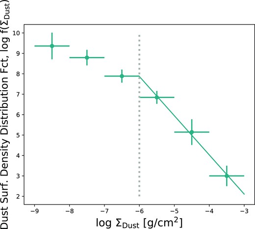
Dust surface density distribution function. This function is computed in analogy with the gas column density distribution function. We note a turnover at low dust surface densities to the left of the dotted grey line. We interpret this feature as due to incompleteness in the sample. Indeed, the data plotted here are focused on the larger N(H i) column density quasar absorbers. We fit the high dust surface density values, log ΣDust ≥ −6, with a simple power law of the form log f(ΣDust) = −1.92 × log ΣDust − 3.65. This observed relation, which can be computed by spatially resolved simulations predicting dust mass functions through 2D projection, provides new constraints on modern dust models.
which we rewrite as
for surface densities with log ΣDust ≥ −6 in units of g cm−2. Here, log f(ΣDust) is the number of systems with dust surface density ΣDust per unit of dust surface density ΔΣDust. It is therefore expressed in number of systems cm2 g−1. C is the normalization factor. The fit is also shown in Fig. 4. Rees (1988) demonstrated that assuming randomly distributed lines of sight through spherical isothermal haloes the column density distribution function, f(N), was shown to have a power law of slope δ = 5/3. Interestingly, Kim, Cristiani & D’Odorico (2001) report a slope δ ∼ 1.5 for H i absorbers and Churchill et al. (2003) and Richter et al. (2011) measure slopes ranging δ = 1.5–2.0 for Mg ii, Fe ii, Mg i, and Ca ii, respectively. Therefore, the slope of the dust surface density distribution function, δ = 1.92 ± 0.13, is possibly steeper than that for neutral gas and on the high end with respect to metal absorbers. Finally, we note that this observed relation, which simulations predicting dust mass function (Millard et al. 2020; Pozzi et al. 2020) will be able to compute through 2D projection, provides new constraints on modern dust models (McKinnon et al. 2017; Graziani et al. 2019; Hou et al. 2019; Li et al. 2019; Baes et al. 2020).
We caution that these UV-depletion results could potentially be incomplete due to observational biases affecting e.g. the dust surface density distribution. For example, in the Milky Way and the Magellanic Clouds, UV sightlines are biased towards the less reddened stars/lower surface densities by the sensitivity of the UV telescopes. Similarly, such effects apply to gamma-ray bursts and quasar samples so that the dustier objects might be missed from the current sample. Several results (Ellison, Murphy & Dessauges-Zavadsky 2009) indicate that these effects are minimum, but one cannot fully exclude that dustier objects exist and have been missed from dust-depletion studies presented here.
4 CONCLUSIONS
In this work, we have looked at an observable, namely ΣDust, to put novel constraints on simulations of dust. Indeed, reproducing dust masses over cosmic times requires that dust grow in the interstellar medium, and therefore that the dust properties change significantly with environment, particularly density. To this end, we gathered observations from the Milky Way, Large and Small Magellanic Clouds, and high-redshift galaxies traced by gamma-ray burst host galaxies and quasar absorbers. By putting all these results together, we can make a new appraisal of the dust surface density (dust column density) expressed in g cm−2 or alternatively in M⊙ kpc−2 across cosmic times measured through dust depletion. We also contrast the observational measurements with recent hydrodynamical simulations. Our main results are as follows:
The dust surface densities increase with cosmic time with a large scatter at any given redshift.
The dust surface densities are also a function of the total gas surface densities in the same systems, with dust surface density increasing with total hydrogen surface density, although the scatter in the relation is four orders of magnitude.
There is a tight correlation between the dust column densities and the dust-corrected metallicity estimates at all cosmic times.
We introduce the dust surface density distribution function – in analogy with the cold gas column density distribution function. We note a turnover at low dust surface densities. We interpret this feature as due to incompleteness in the sample. We provide a fit to the observed distribution of the form log f(ΣDust) [number of systems per unit dex] = −1.92 × log ΣDust − 3.65, which proves steeper than that for neutral gas and metal absorbers.
SUPPORTING INFORMATION
suppl_data
Please note: Oxford University Press is not responsible for the content or functionality of any supporting materials supplied by the authors. Any queries (other than missing material) should be directed to the corresponding author for the article.
ACKNOWLEDGEMENTS
We are grateful to Omima Osman, Enrico Garaldi, Qi Li, Julia Roman-Duval, and Sandra Savaglio for helpful comments. We thank the anonymous referee for their suggestions that improved the results presented here. This research was supported by the International Space Science Institute (ISSI) in Bern, through ISSI International Team project #564 (The Cosmic Baryon Cycle from Space). ADC acknowledges support from the Swiss National Science Foundation under grant 185692. JCH recognizes support from the US National Science Foundation through grant AST-1910255.
DATA AVAILABILITY
Data directly related to this publication and its figures are available on request from the corresponding author.
References
APPENDIX A: OBSERVED DUST PROPERTIES AT VARIOUS COSMIC TIMES
Table A1 lists the observed physical properties of different environment plotted in Figs 1–3. We derive these quantities from data of the Milky Way (De Cia et al. 2021), the Large and Small Magellanic Clouds observations (Roman-Duval et al. 2022a), the gamma-ray bursts information (Bolmer et al. 2019b), and the quasar absorbers data (Péroux & Howk 2020). This extract shows the first few entries while the full table is available as machine-readable online material.
Summary of the observational data used in this study. The first column refers to the systems under study, the second column lists our computation of the logarithm of the dust surface density in units of g cm−2, the third column provides the redshift, while the fourth column tabulates the total gas surface density and the last column provides the dust-depletion corrected total metallicity with respect to solar.
| System | log ΣDust | Redshift | log ΣGas | Metallicity |
|---|---|---|---|---|
| (g cm−2) | (g cm−2) | [M/H]total | ||
| Milky Way | −5.05 ± 0.61 | 0.000 | −2.49 ± 0.20 | −0.39 ± 0.18 |
| Milky Way | −5.04 ± 0.52 | 0.000 | −2.31 ± 0.20 | −0.56 ± 0.09 |
| Milky Way | −5.48 ± 0.55 | 0.000 | −3.12 ± 0.20 | −0.18 ± 0.13 |
| Milky Way | −4.87 ± 0.56 | 0.000 | −2.33 ± 0.20 | −0.41 ± 0.13 |
| Milky Way | −4.81 ± 0.62 | 0.000 | −2.12 ± 0.20 | −0.50 ± 0.20 |
| Milky Way | −5.35 ± 0.56 | 0.000 | −3.46 ± 0.20 | +0.28 ± 0.13 |
| ... |
