


ABSTRACT
In this work, we report the presence of rapid intra-night optical variations in both flux and polarization of the blazar BL Lacertae during its unprecedented 2020–2021 high state of brightness. The object showed significant flux variability and some colour changes, but no firmly detectable time delays between the optical bands. The linear polarization was also highly variable in both polarization degree and angle (electric vector polarization angle). The object was observed from several observatories throughout the world, covering a total of almost 300 h during 66 nights. Based on our results, we suggest that the changing Doppler factor of an ensemble of independent emitting regions, travelling along a curved jet that at some point happens to be closely aligned with the line of sight, can successfully reproduce our observations during this outburst. This is one of the most extensive variability studies of the optical polarization of a blazar on intra-night time-scales.
1 INTRODUCTION
BL Lacertae is the archetype of the blazar-class objects, a class of active galactic nuclei, which can generally be characterized by two main features: (i) almost entirely non-thermal continuum spectrum in the complete electromagnetic (EM) bands, stretching up to 15 orders of magnitude on the frequency scale, with a characteristic broad bimodal spectral energy distribution (SED; e.g. Fossati et al. 1998; Abdo et al. 2010b) and (ii) intermittent flux, spectral and polarization variability in all bands and on all time-scales, from minutes to years (e.g. Miller, Carini & Goodrich 1989; Raiteri et al. 2009, 2010, 2013; Gaur et al. 2014, 2015a, b; Agarwal & Gupta 2015; D’Ammando 2022; Imazawa et al. 2023; Sahakyan & Giommi 2022; Hazama et al. 2022, and references therein). The lower energy part of the SED is dominated by synchrotron radiation but the high-energy part of SED remains in question. High-energy portion of SED is generally explained by leptonic models, e.g. synchrotron self-Compton or external Compton, and alternate hadronic models are preferable for some sources (e.g. Gao et al. 2019; Böttcher et al. 2013, and references therein). From the composite UV/optical spectral perspective, blazars are divided into two classes: BL Lacertae objects (BLLs) and flat-spectrum radio quasars (FSRQs), depending on whether they show prominent emission lines and/or thermal accretion disc signatures (latter) or not (former). In addition to an apparent correlation between the frequency at which the two humps of the SED peak, as well as its correlation with luminosity (Fossati et al. 1998), an SED-based classification has been argued that designates a blazar based on the frequency (|$\nu _{\mathrm{ syn}}^{\mathrm{ peak}}$|) at which synchrotron part (low-energy hump) peaks. If |$\nu _{\mathrm{ syn}}^{\mathrm{ peak}} \le 10^{14}$| Hz, the blazars are called low synchrotron peaked (LSPs), if |$10^{14} \le \nu _{\mathrm{ syn}}^{\mathrm{ peak}} \le 10^{15}$| Hz then called intermediate synchrotron peaked, and if |$\nu _{\mathrm{ syn}}^{\mathrm{ peak}} \ge 10^{15}$| Hz then known as high synchrotron peaked (HSPs; Abdo et al. 2010b). The commonly accepted understanding, however, is that all blazars possess a strong relativistic jet that happens to be pointed almost directly towards the observer’s line of sight (Urry & Padovani 1995), and which produces most of the energy via non-thermal processes. This energy, covering practically the entire observable EM spectrum, is additionally Doppler boosted towards the observer, as being generated along a relativistic jet, which significantly amplifies the fluxes and shortens the characteristic variability time-scales. Therefore, it is not surprising to observe significant (say 10 per cent) optical/gamma variations for as short as ∼15 min occasionally in some of these objects (e.g. Ulrich, Maraschi & Urry 1997).
It is not yet clear why, but the FSRQs (and perhaps some LSP BLLs) statistically turn out to be more variable on both intra-night and long-term time-scales in optical bands than the HSP BLLs, as the former show faster and more prominent variations (e.g. Bachev 2018, and references therein). The explanation of this tendency, if further confirmed, could probably be looked for in terms of the jet-producing mechanisms – being based on the extraction of energy of the black hole spin (Blandford & Znajek 1977) or on the accretion disc itself (Blandford & Payne 1982).
BL Lacertae, located at a cosmological redshift of z = 0.069 (MacLeod & Andrew 1968; Schmitt 1968; Oke & Gunn 1974), is a prototype of BL Lacertae class of sources, which were first identified as sources with peculiar spectra and strong and rapid flux variability in radio and optical bands (e.g. Moore et al. 1982; Miller et al. 1989; Fan et al. 1998; Hagen-Thorn et al. 2002; Agarwal & Gupta 2015, and references therein). The perplexing behaviour of flux variations on time-scales of a few hours to within a day, now widely referred in the literature as intra-night (or intra-day, IDV) variability (Wagner & Witzel 1995) feature, has been reported even in the very early optical observations (e.g. DuPuy et al. 1969; Racine 1970; Miller et al. 1989), and has now become one of the identifying criteria for blazars. Since then, the source has been an extensively observed and explored source across the EM spectrum, independently as well as in a coordinated ways (Miller et al. 1989; Fan et al. 1998; Raiteri et al. 2009, 2010, 2013; Agarwal & Gupta 2015; Gaur et al. 2015a, b; MAGIC Collaboration 2019; Weaver et al. 2020). These studies reveal not only strong flux and polarization variability, but also significant spectral changes, especially in the X-ray band (e.g. Raiteri et al. 2009). The anticorrelated optical flux and degree of polarization are detected in the source in 2008–2009 observing season (Gaur et al. 2014). In the historic and unprecedented optical activity of 2020–2021 (Kunkel et al. 2021; Marchini et al. 2021), an extremely soft X-ray spectrum was seen (e.g. Prince 2021, and references therein), a transition similar to that of another BL Lac object OJ 287 (e.g. Kushwaha et al. 2018; Kushwaha 2022). This historic activity was followed in all the EM bands (e.g. Marchini et al. 2021; Jorstad et al. 2022; Prince 2021, and references therein), and we too monitored the source optical brightness and polarization intensively and extensively. Recently, an ∼13-h optical quasi-periodic oscillation is reported in BL Lacerate in its observations in the historical pre-outburst in 2020 (Jorstad et al. 2022). In another recent optical flux and spectral variability study carried out during this historical outburst, IDVs with an amplitude up to ∼30 per cent were detected, and the spectral evolution was predominated by flattening of the spectra with increasing brightness, i.e. a bluer-when-brighter (BWB) trend was observed (Kalita et al. 2022).
In this paper, we present the intra-night optical (flux and polarimetric) variability study of BL Lacertae during its year 2020–2021 optical maximum, unsurpassed for at least 15 yr (see e.g. Tuorla monitoring programme,1 St. Petersburg monitoring programme,2 etc.). The object reached R ≃ 11.5 mag at some point (Kunkel et al. 2021; Marchini et al. 2021), a historical maximum that has never been reported before, at least what concerns the last few decades. The studies in the optical region are important, as often there the synchrotron peak is located (at least for LSPs). The strong intra-night variability is a well-documented and studied feature in many blazars, including BL Lacertae (e.g. Miller et al. 1989; Papadakis et al. 2003; Stalin et al. 2006; Zhai & Wei 2012; Agarwal & Gupta 2015; Gaur et al. 2015b; Bhatta & Webb 2018; Fang et al. 2022; Imazawa et al. 2023, and references therein).
Despite the significant progress throughout the years, yet no entirely consistent picture has emerged to be able to account for all observational signatures. On the other hand, the physics of the relativistic jets can be really complicated and can include processes such as standing or propagating shocks; blobs or ‘plasmoids’, moving along the jet; relatively ordered (helical) or highly disordered (turbulent) magnetic fields, etc., all of which can, one way or another, influence the synchrotron emission, even on intra-night time-scales. In addition, the Doppler-boosting factor is another major ‘modifier’ of the emission, capable of significantly (and non-linearly) increasing the flux intensity in the observer’s frame of reference (e.g. Böttcher et al. 2013; Marscher 2014, 2015; Zhang, Chen & Böttcher 2014; Zhang et al. 2015, and references therein). Therefore, a systematic study of the intra-night variability of a blazar can significantly help to improve the existing models, especially when colour and polarimetric variations are also simultaneously investigated. Our main goal will be to study how during the maximum light of BL lacerate the intra-night activity changes with the average brightness in the optical band. We search for intra-night colour changes, study changes in the polarization rate and the orientation of the electric vector (electric vector polarization angle, EVPA), and search for relations among different temporal characteristics of the intra-night variations. To the best of our knowledge, this is one of the first time the polarimetric variability of this blazar is systematically studied on intra-night time-scales. Recently, similar studies exploring intra-night photopolarimetric variability of BL Lacerate in which the source has also shown significant flux and polarimetric variations were reported (Imazawa et al. 2023; Shablovinskaya et al. 2023).
In this paper, we concentrate only on the short-term (intra-night) variability of BL Lacertae. The long-term flux and polarization variability results, covering this exceptional period, will be published elsewhere (Raiteri et al. 2023).
The paper is structured as follows: In Section 2, we provide observations carried out from different telescopes and their data analysis. Results are reported in Section 3. The discussion and conclusion are provided in Sections 4 and 5, respectively.
2 OBSERVATIONS AND DATA ANALYSIS
BL Lacertae was monitored for intra-night variability during 66 nights for a total of almost 300 h throughout the years 2020–2021. Thus, the average monitoring duration was about 4 h, but ranged from about 1 to more than 8 h. In addition, data from other 24 nights (about 73 h), taken between years 2017 and 2019, when the blazar was not in a maximum state, were also analysed. A sample of log of observations is shown as Table 1, whereas a complete list is presented in Table A1.
A sample of observational log. The complete observation log is given in Table A1.
| JD | Evening | Telescope | Duration | Filters | <R> | σ(R) | <V − I> |
|---|---|---|---|---|---|---|---|
| 245 8011.35 | 14.9.17 | B60 | 4.6 | BVRI | 13.150 | 0.020 | 1.45 |
| 245 8012.35 | 15.9.17 | B60 | 4.0 | BVRI | 13.250 | <0.005 | 1.44 |
| 245 8341.46 | 10.8.18 | B60 | 2.7 | BVRI | 12.900 | 0.010 | 1.38 |
| 245 8343.44 | 12.8.18 | B60 | 2.5 | BVRI | 13.500 | 0.010 | 1.41 |
| 245 8344.43 | 13.8.18 | B60 | 4.0 | BVRI | 12.940 | 0.020 | 1.38 |
The observations were performed with several small- and middle-class telescopes, such as 2-m RCC telescope of Rozhen National Observatory3 (Bulgaria), 0.6-m telescope of Belogradchik Observatory4 (Bulgaria), 1.3-m telescope of Skinakas Observatory5 (Greece), 1.04-m telescope of ARIES6 Nainital (India), and 1.4- and 0.6-m telescope of Vidojevica Observatory7 (Serbia). All telescopes were using CCDs, equipped with standard (Johnson–Cousins) UBVRI broad-band filter sets. Additionally, the Belogradchik 0.6-m telescope was equipped with a double-barrel filter set, made by FLI, allowing a combination of UBVRI with polarimetric filters, thus making possible to perform a linear polarimetry of the blazar in the optical band selected. We also used the FoReRo-2 mode of the 2-m Rozhen telescope, allowing a beam splitting between the red and blue channels, thus allowing simultaneous exposures in both channels, using two separate (blue- and red-sensitive) CCDs.
All frames thus collected were properly reduced (flat-field, bias, dark frame – where applicable) and an aperture photometry was performed in order to extract the magnitudes. The photometric measurements were made with respect to the standard stars B, C, and H with an aperture radius of 8 arcsec, as suggested by the GLAST-AGILE Support Program (GASP) consortium,8 and the BVRI magnitudes of these standard stars are taken from Bertaud et al. (1969) and Fiorucci & Tosti (1996). The (quasi-)simultaneous multicolour observations were made via taking BVRI frames in a consecutive order (Skinakas, Belogradchik, and Vidojevica) or by using a beam splitter, allowing simultaneous BR observations (Rozhen). Note that for an exposure time of 60–120 s, the combined time resolution of the light curves (LCs) in the former approach could not be shorter than 5 min and was typically less than 1 min in the latter. The details about telescopes, CCDs, filter systems, and photometric data analysis are provided in our series of papers (e.g. Strigachev & Bachev 2011; Bachev et al. 2012, 2017; Gaur et al. 2012a; Gupta et al. 2017a, 2019; Pandey et al. 2020).
Three polarimetric filters (oriented at 0–180, 60–240, and 120–300 deg) were used to obtain the polarization degree (p) and the EVPA. This approach obviously could not employ the standard Stokes parameters and requires instead solving three equations for three unknowns (Bachev 2023):
|$I_{\rm 0}=\frac{1}{2}I_{\rm np}+I_{\rm p}\cos ^{2}\theta$|
|$I_{\rm 60}=\frac{1}{2}I_{\rm np}+I_{\rm p}\cos ^{2} (\theta -60)$|
|$I_{\rm 120}=\frac{1}{2}I_{\rm np}+I_{\rm p}\cos ^{2} (\theta -120)$|, where
|$p[{{\rm per\ cent}}]=100\frac{ I_{\rm p}}{ I_{\rm np}+ I_{\rm p}}$|, and EVPA = θ.
We solved these equations numerically. For each orientation, at least three, but normally five, frames were taken, in a consecutive order, and the standard deviation of the object’s magnitude among these frames was taken as a proxy of the photometric error. Note that any intrinsic variability (the typical polarization exposure time was 120 s) in between the frames will only artificially increase this error. Unfortunately, this is the limitation of our apparatus. The errors of p and EVPA were obtained by varying the obtained magnitudes in each orientation within their respective photometric errors. For the magnitudes, a Gaussian distribution was assumed, which is approximately correct; however, the polarization parameters are certainly not Gaussian distributed (p is not even symmetrically distributed); i.e. the errors presented in Fig. 6 and Table 2 are just the standard deviations. All polarimetric measurements were made in the R band only.
Polarimetric results (observations only in the R band).
| JD | Evening | Duration | <p> | <Err(p)>a | σ(p) | Probability | <EVPA> | <Err(EVPA)> | σ(EVPA) | Probability |
|---|---|---|---|---|---|---|---|---|---|---|
| dd.mm.yy | (h) | (per cent) | (per cent) | (per cent) | (deg) | (deg) | (per cent) | |||
| 245 9112.27 | 19.09.20 | − | 9.3 | 0.5 | − | − | 30.4 | 1.7 | − | − |
| 245 9113.29 | 20.09.20 | − | 7.9 | 0.7 | − | − | 24.5 | 2.2 | − | − |
| 245 9114.28 | 21.09.20 | − | 11.2 | 0.3 | − | − | 23.6 | 0.6 | − | − |
| 245 9115.30 | 22.09.20 | − | 8.4 | 1.1 | − | − | 26 | 0.8 | − | − |
| 245 9116.35 | 23.09.20 | − | 8 | 0.4 | − | − | 27.9 | 1.4 | − | − |
| 245 9117.28 | 24.09.20 | − | 6.7 | 0.3 | − | − | 12 | 1.8 | − | − |
| 245 9134.25 | 11.10.20 | − | 4.8 | 0.4 | − | − | 24.8 | 4.3 | − | − |
| 245 9141.29 | 18.10.20 | − | 8.2 | 0.8 | − | − | 6.7 | 2.9 | − | − |
| 245 9142.29 | 19.10.20 | − | 4.5 | 0.5 | − | − | 1.8 | 3.8 | − | − |
| 245 9143.29 | 20.10.20 | − | 6.7 | 0.7 | − | − | 167.9 | 2.1 | − | − |
| 245 9144.24 | 21.10.20 | − | 6.1 | 0.8 | − | − | 29.2 | 4.1 | − | − |
| 245 9145.26 | 22.10.20 | − | 10.1 | 0.5 | − | − | 10.2 | 1.3 | − | − |
| 245 9161.44 | 07.11.20 | − | 11.6 | 0.8 | − | − | 12.9 | 2.2 | − | − |
| 245 9386.48 | 20.06.21 | − | 5.9 | 0.4 | − | − | 57.8 | 2.2 | − | − |
| 245 9403.51 | 07.07.21 | 2.4 | 15.2 | 0.7 | 2.0 | >99.999 | 11.2 | 1.5 | 1.4 | >90 |
| 245 9404.51 | 08.07.21 | 2.3 | 12.9 | 0.4 | 0.5 | <90 | 10.9 | 1.1 | 0.4 | <90 |
| 245 9406.52 | 10.07.21 | 1.9 | 5.1 | 0.5 | 1.0 | >99.9 | 9.1 | 2.1 | 3.3 | >99 |
| 245 9407.49 | 11.07.21 | 4.0 | 8.4 | 0.6 | 1.5 | >99.999 | 9.6 | 2.6 | 5.6 | >99.999 |
| 245 9408.42 | 12.07.21 | 0.5 | 16.2 | 1.1 | 2.3 | >95 | 0.8 | 1.0 | 0.6 | <90 |
| 245 9434.45 | 07.08.21 | 5.6 | 5.2 | 0.4 | 1.1 | >99.999 | 178.2 | 3.0 | 2.7 | >90 |
| 245 9435.46 | 08.08.21 | 5.7 | 12.7 | 0.5 | 1.1 | >99.999 | 10.7 | 1.3 | 2.2 | >99.999 |
| 245 9436.50 | 09.08.21 | 5.5 | 8.2 | 0.9 | 1.5 | >99.99 | 18.9 | 3.3 | 6.8 | >99.999 |
| 245 9437.45 | 10.08.21 | 5.9 | 2.5 | 0.4 | 0.9 | >99.999 | 2.5 | 6.8 | 7.0 | >90 |
| 245 9438.43 | 11.08.21 | 5.1 | 8.9 | 0.6 | 1.8 | >99.999 | 156.6 | 1.8 | 3.7 | >99.999 |
| 245 9439.44 | 12.08.21 | 5.4 | 7.2 | 0.4 | 0.9 | >99.999 | 146.9 | 1.8 | 1.9 | >99 |
| 245 9440.42 | 13.08.21 | 5.6 | 7.2 | 0.5 | 0.6 | >99.9 | 149.3 | 1.9 | 2.9 | >99.999 |
| 245 9443.54 | 16.08.21 | 2.0 | 4.4 | 0.5 | 1.0 | >99.99 | 160 | 4 | 9.0 | >99.999 |
| 245 9468.42 | 10.09.21 | 8.0 | 4.2 | 0.4 | 0.7 | >99.999 | 87.2 | 3.4 | 9.2 | >99.999 |
| 245 9469.43 | 11.09.21 | 7.8 | 8.4 | 0.4 | 1.2 | >99.999 | 56.9 | 1.9 | 2.8 | >95 |
| 245 9470.43 | 12.09.21 | 8.1 | 10.4 | 0.5 | 1.0 | >99.999 | 69.7 | 1.5 | 3.9 | >99.999 |
| 245 9471.42 | 13.09.21 | 8.1 | 4.3 | 0.6 | 0.9 | >99.999 | 72.6 | 4.4 | 16.3 | >99.999 |
| 245 9472.40 | 14.09.21 | 6.3 | 6.2 | 0.8 | 0.6 | >99 | 85.4 | 3.6 | 5.7 | >99.999 |
| 245 9473.40 | 15.09.21 | 6.9 | 4.6 | 0.5 | 1.1 | >99.999 | 108.4 | 3.0 | 9.7 | >99.999 |
| 245 9520.34 | 01.11.21 | 6.4 | 14.5 | 0.4 | 0.5 | >95 | 30.3 | 0.6 | 0.8 | >99.9 |
| 245 9604.21 | 24.02.22 | − | 11.6 | 0.5 | − | − | 26.3 | 1.1 | − | − |
Standard deviations, as mentioned in Section 2.
3 RESULTS
3.1 Intra-night variability
Tables 1, A1, and 2 summarize the results of our optical photometric and polarimetric monitoring of BL Lacertae. The figures (Figs 1–4) show examples of prominent variations on intra-night time-scales. The upper panel of each figure shows the LCs in one or more filter bands for the different instruments. The magnitudes of some bands have been arbitrarily shifted for presentation purposes. Again, for presentation purposes no photometric errors were shown; however, during this very bright state, they all were typically <0.01 mag (<0.02 mag for the B band, for the smallest Belogradchik and Vidojevica telescopes). In other photometric bands, i.e. VRI, we have even lesser errors than the B band. The evening date of each observation is indicated.
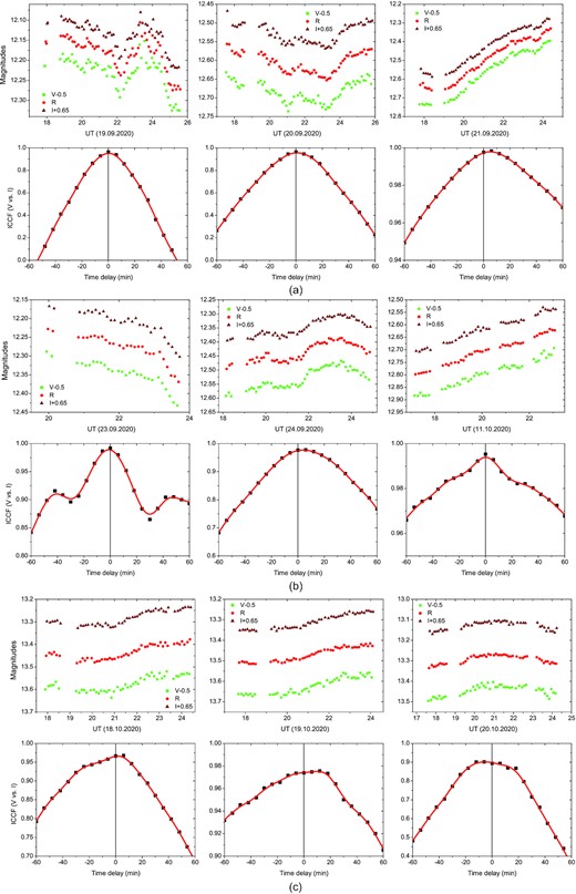
Quasi-simultaneous (repeating VRI filters) intra-night LCs of BL Lacertae with the 60-cm Belogradchik telescope. Each lower panel shows the ICCF between V and I bands (positive time delay means that V is leading). All pronounced ICCF peaks appear to coincide with zero lag (at least within the time resolution of about 6 min for this instrument).
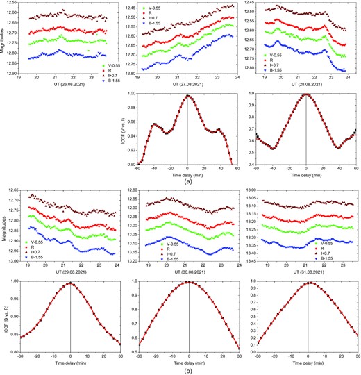
Examples of quasi-simultaneous intra-night monitoring (BVRI) with the 1.3-m Skinakas telescope. Due to the lack of prominent variability, no cross-correlation of the LCs has been attempted for the night of 2021 August 26. Here, B versus R are used to search for time delays. No such time delays are evident from our data.
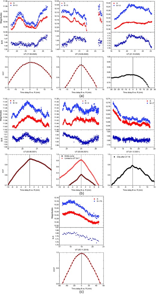
Examples of simultaneous BR monitoring with 2-m Rozhen telescope. Clearly, BL Lacertae shows short-lasting small-scale micro variations of one or two hundreds of a magnitude, well visible in both bands. The B − R colour (the middle panel of each night) also shows small-scale changes, which do not seem to be highly correlated with the flux level. The ICCFs are generally peaking at zero (within 1 min), at least when the peaks are well defined.
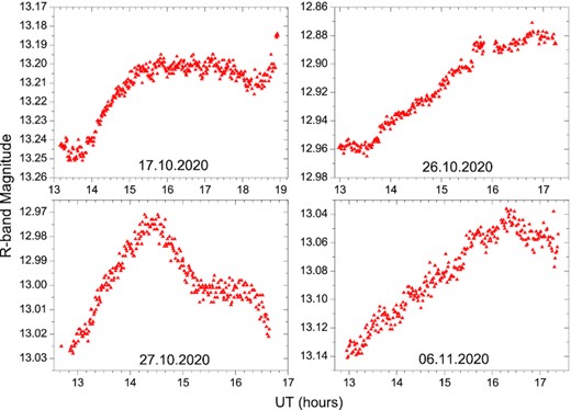
Examples of R-band intra-night monitoring with the 1-m ARIES telescope.
One sees significant intra-night variability, at least during the periods of high-flux states. All bands show unpredictable, but systematic behaviour among them. Variations sometimes reach up to 0.3 mag within several hours of observations (e.g. the night of 2020 September 21, Fig. 1a), and can be as rapid as ∼0.1 mag for half an hour (e.g. 2021 August 28, Fig. 2a). To explore intra-night variability, we exploited two of the most widely used methods: power-enhanced F-test (de Diego 2014; de Diego et al. 2015) and nested analysis of variance (ANOVA; de Diego et al. 1998, 2015) as detailed below. An intra-night LC is reported to be variable only if it is found variable by both enhanced F-test and nested ANOVA test.
3.1.1 Power-enhanced F-test
The power-enhanced F-test is introduced by de Diego (2014) and de Diego et al. (2015). We use one comparison star as reference star to find the differential light curves (DLCs) of the blazar and other comparison stars. The variance of blazar LC is compared with the combined variance of comparison stars. It is defined as (Pandey et al. 2019)
where |$s^2_{\mathrm{ blz}}$| is the variance of the DLCs of difference of instrumental magnitude of blazar and reference star, and
and is defined as the variance of the combined DLCs of difference of instrumental magnitude of comparison star and reference star. Nj is the number of data points of the j-th comparison star, and |$s^2_{j,i}$| is its scaled square deviation, which is defined as
where ωj, mj, i, and |$\bar{m}_j$| are scaling factor of j-th comparison star DLC, its differential magnitude, and its mean magnitude, respectively. The averaged square error of the blazar DLC divided by the averaged square error of the j-th comparison star is used as the scaling factor.
In this work, we have three comparison stars B, C, and H. As BL Lacertae magnitude was closest to the comparison star C, we have taken C as the reference star. Since two more comparison stars are left, k = 2. The blazar and all the comparison stars have the same number of observations N, so the degree of freedom in the numerator is (N − 1) and the denominator is k(N − 1). We have found Fenh using equation (1) and compared it with Fc at the confidence level of 99 per cent, i.e. α = 0.01. If Fenh > Fc, then DLC is considered as Variable (V); otherwise, it is considered as Non-Variable (NV).
3.1.2 Nested ANOVA test
For active galactic nucleus (AGN) variability, the one-way ANOVA test was introduced by de Diego et al. (1998). The nested ANOVA test is an updated version of the ANOVA test (de Diego et al. 2015). In nested ANOVA test, we use all the comparison stars as reference stars to find the DLCs. Unlike power-enhanced F-test that needed one comparison star, here we are using all the comparison stars as reference stars, so we have one more star to work with. We have three comparison stars in this work, namely B, C, and H to generate the DLCs of the blazar. We group these DLCs in such a way that we have five points in each group. From equation (4) of de Diego et al. (2015), we have estimated the values of MSG (mean square due to groups) and MSO(G) (mean square due to nested observations in groups). We then estimated the F-statistics using the ratio F = MSG/MSO(G). At a confidence level of 99 per cent, i.e. α = 0.01, if F-statistics >FC then we say that LCs are variable (V); otherwise, we say it is non-variable (NV). The sample and detailed results of power-enhanced F-test and nested ANOVA test are given in Table 3 and Table B1, respectively.
A sample result of IDV of BL Lac. The complete results of IDV are provided in Table B1.
| Obs. date | Obs. start time | Band | Power-enhanced F-test | Nested ANOVA | Variability | A | ||
|---|---|---|---|---|---|---|---|---|
| dd-mm-yyyy | JD | DoF(ν1, ν2) | Fenh/Fc | DoF(ν1, ν2) | F/Fc | status | (per cent) | |
| 2017-09-14 | 245 8011.269 80 | V | 38, 76 | 2.27/1.87 | 9, 30 | 38.47/3.06 | V | 8.22 |
| 245 8011.265 39 | R | 39, 78 | 4.12/1.86 | 9, 30 | 41.78/3.06 | V | 7.84 | |
| 245 8011.266 85 | I | 40, 80 | 2.26/1.84 | 9, 30 | 20.84/3.06 | V | 8.86 | |
3.1.3 Intra-night variability amplitude
For each of the intra-night variable LCs, we estimated the percentage of variability amplitude (A), using the equation provided by Heidt & Wagner (1996).
where Amax and Amin are the maximum and minimum magnitudes in a variable LC, respectively, and σ is the mean error of the LC. The amplitude of variability is reported in the last column of Table 3 and Table B1.
3.2 A light-curve comparison
Fig. 5 presents a comparison of two R-band measurements, obtained by two different telescopes (Rozhen 2-m and Belogradchik 0.6-m), during the same night – 2020 September 20. Clearly the match is impressive, even taking into account the different equipment used in these telescopes, the different altitudes and probably atmospheric conditions, etc.; no shifts were needed to match the LCs. Such a comparison allows judging on the reliability of our results.
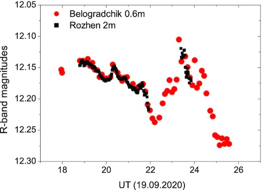
Comparison of the R-band LC of BL Lacertae, obtained with two different instruments, equipped with different CCDs and filter sets. The close match seen in the figure is indicative of the reliability of our photometry.
3.3 Colour changes
The changes of colour (directly related to the source spectrum) are a well-documented feature of the blazars’ optical SED. BL lac-type objects, such as BL Lacertae, are known to show a general ‘BWB’ behaviour (e.g. Gu et al. 2006; Gaur et al. 2012b; Bhatta & Webb 2018, and references therein). Colour changes on the intra-night time-scales are rarely studied (e.g. Agarwal & Gupta 2015) but a genuine colour change has been rarely reported for this object (e.g. Imazawa et al. 2023; Kalita et al. 2022). Our results clearly demonstrate the presence of a low-level colour change, for a period of a few hours. The second panels of Fig. 3 show the colour variability. It is clearly seen during some nights (e.g. 2020 October 21, 2021 September 3, etc.). Fig. 7 indicates a BWB behaviour for the averaged values during each observing night, which, as mentioned above, is expected for this type of objects.
3.4 Time lags
Multiband monitoring allows searching for possible time delays among the bands. Unfortunately, repeating exposures in consecutive filters limits the time resolution of possible time-delay detection. Any detected delays, shorter than the time between two image frames of the same band, should be considered unreliable. In our monitoring, the typical data recording at Belogradchik 0.6-m were ∼6 min, Skinakas 1.3-m ∼3 min, and Rozhen 2-m ∼1 min. The other instruments either did not observe in multiple bands or lacked significant variability to perform this test.
To search for time delays, we employed the interpolated cross-correlation function (ICCF), a method proposed by Gaskell & Sparke (1986) and widely used afterward to study the correlations between unevenly sampled time series data. This method uses a linear interpolation between the adjacent data points, to account for unevenly sampled data, different exposure times, and generally the lack of a temporal match between the corresponding points from the two LCs (data sets) that are to be cross-correlated. Thus, the ICCF is being built as a function of the time shift between the curves. The time shift – τ (positive or negative), at which ICCF(τ) reaches maximum, gives the time delay between the curves. Normally, a positive τ indicates that the first LC is leading the second one. ICCF method is suitable for our case, as the data points are almost equidistant; i.e. there are typically no large missing portions of the intra-night LC to be replaced by straight lines.
The time-delay results are shown in the lowest panels of Figs 1, 2, and 3. For the different telescopes, depending on their equipment in use, we compared the optical bands with the highest signal-to-noise ratio and the LCs providing the highest time resolution. Based on our results, we cannot claim any securely detected time delays. Although some indications for such delays are evident (e.g. 2020 September 21, Fig. 1a, and 2021 August 31, Fig. 2b), first, the results do not appear to be systematic and secondly, the delays are typically within the time resolution, as mentioned above.
3.5 Polarimetric variability
The synchrotron radiation is naturally linearly polarized, with a polarization degree that can in theory exceed 50 per cent under the right circumstances (Rybicki & Lightman 1986). Until recently, the common understanding, however, was that both polarization rate and the EVPA are rather stable, or at least not highly variable on intra-night time-scales. At least during the high-activity episodes, this notion, however, does not seem to hold true. For instance, Bhatta & Webb (2018) reported significant polarization variability within several hours, during a strong optical micro-flare of S5 0716+714. In a multiwavelength (γ-ray, optical flux, and polarization, plus Very Long Baseline Array) observation of S5 0716+714, Larionov et al. (2013) reported a rapid rotation of the linear polarization coincident with the flare peak in both optical flux and γ-ray and a new superluminal radio knot appeared essentially at the same time (Chandra et al. 2015). In 3C 279, during a multiwavelength observational campaign from 2008 to 2009, Abdo et al. (2010a) reported a γ-ray flare coincident with a dramatic change of optical polarization angle. On another occasion, high γ-ray activity of 3C 279 in 2011 showed multiple peaks and coincided exactly with a 352° rotation of the optical polarization angle and flaring activity at optical bands (Kiehlmann et al. 2016). In 3C 454.3, a peculiar optical polarization behaviour was reported during 2009 December 3–12 high multiwavelength activity. A strong flare peaking in γ-rays, X-rays, and optical/near-infrared almost at the same time showed a strong anticorrelation between optical flux and degree of polarization and a large rapid swing in polarization angle of 170° (Gupta et al. 2017b). There are several studies of optical polarization variability of blazars on diverse time-scales that have shown that virtually all blazars studied are polarimetrically variable on all possible time-scales, i.e. intra-night, short as well as long (e.g. Andruchow et al. 2003, 2011; Andruchow, Romero & Cellone 2005; Ikejiri et al. 2011; Bhatta et al. 2016; Sosa et al. 2017; Marscher & Jorstad 2021; Hazama et al. 2022; Imazawa et al. 2023, and references therein).
The results of our intra-night polarimetric variability are shown in Table 2 and Fig. 6. We employed the χ2 statistics in order to quantify the reality of the variations in both polarization degree and EVPA. For comments on χ2 and comparison among other similar approaches, see e.g. de Diego (2010). First, we calculated χ2 and the right-tailed probability P(χ2, n) of the χ2 distribution as
|$\chi ^{2}=\sum _{i=1}^{N}\frac{(y_{i}-f(x_{i}))^{2} }{\sigma _{i}^{2}},$|
|$P(\chi ^{2}, n)=\frac{2^{-n/2}}{\Gamma (n/2)} \chi ^{n-2} e^{-\chi ^2/2}.$|
We used the weighted-average χ2 approach, as described by de Diego (2010, and the references therein); i.e. f(x) = 〈y〉 is the weighted average of the measured values. Then, we used the chi-square value to calculate the probability that the deviations are not due to random variations, i.e. calculated 1 − P(χ2, n). Here, n is the degrees of freedom; in our case, n = N − 1, where N is the number of observations.


Intra-night multicolour and R-band polarimetric observations with the 60-cm Belogradchik telescope. BVRI LCs (top panel) are shown together with polarization rate (middle panel) and EVPA (bottom panel) for each night. Significant variability in both flux and polarimetric parameters can be seen. These variations do not seem to be correlated in any way.
As seen from the results, at least one of these parameters showed statistically significant changes during virtually every night of monitoring. The most impressive cases include the night of 2021 September 13 (Fig. 6e), when EVPA changed by about 50 deg over 8–9 h, the night of 2021 August 11, when the polarization rate changed by about 5 per cent within a few hours, etc. Note that changes in the polarization parameters do not seem to be related to the changes of the overall flux; i.e. significant optical changes are often not accompanied by polarimetric changes of a similar scale (e.g. the night of 2021 August 9, Fig. 6b) and vice versa.
3.6 The ‘rms–flux’ relation
The large amount of data acquired during the 2020–2021 and the previous campaigns allowed studying the ‘fractional variability–average flux’ or ‘root-mean-square (rms)9–flux’ relation on intra-night time-scales. This relation shows how variable an object is at different flux levels. It has been shown for many accreting objects that their variability is flux dependent (e.g. Bachev et al. 2017, and the references therein). Fig. 7 shows the relation between the rms and the average flux we found for BL Lacertae, as well as the relations among other measurable, like colour, average polarization degree, etc. Since the typical blazar variability structure function (Simonetti, Cordes & Heeschen 1985) is still rising on intra-night time-scales, it is justifiable to use in addition a time-normalized rms, i.e. rms(〈t〉/ttot), where ttot is the time duration of the data set for the corresponding night and 〈t〉 is the average duration of all data sets, which in our case is 4.05 h (more details in Bachev 2015; Bachev et al. 2016, 2017). Thus, the influence of the length of the observation on the rms value will be minimized. Fig. 7 shows, however, that there is no significant difference in which one of those two parameters is used. Both of them show a slight tendency to increase with the average flux. Similar results have been shown to hold true for other blazars as well: CTA 102 (Bachev et al. 2017), S4 0954+65 (Bachev et al. 2016), etc. On the other hand, neither the average flux level nor the rms seems to correlate significantly with the average polarization degree. A peculiar result for BL Lacertae was found in its optical LC where the flux strongly anticorrelated with the degree of optical polarization while the angle of polarization stayed essentially unchanged (Gaur et al. 2014). To explain this peculiar behaviour of BL Lacertae, Gaur et al. (2014) used the AGN model within the framework of a shock wave propagating along a helical path in the blazar’s jet that can explain the variety of flux and polarization patterns in blazars LCs (Marscher et al. 2008; Larionov et al. 2013).
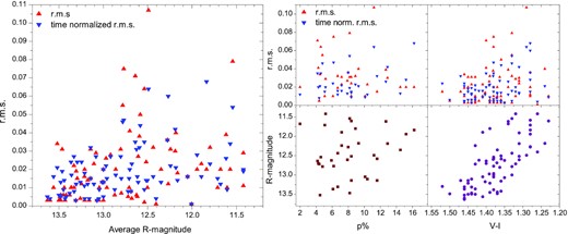
Statistical dependences on intra-night time-scale. Left-hand panel: The relation between the variability rate (rms) and the average R-band magnitude. Clearly, a tendency for higher fractional variability during episodes of higher flux levels is evident. The right-hand panel shows relations among the flux, the colour, the rms, and the polarization degree. No clear dependences are seen, except for the colour–magnitude relation (BWB), which is expected for such types of blazars.
4 DISCUSSION
Although intra-night variability is now a characteristic feature of identifying blazars, a detailed explanation of this intra-night variability, often being as rapid as tenths of magnitude in a matter of minutes, is still under debates. Such short characteristic times limit the size of the active region that produces the observed emission and suggest the presence of an ensemble of relatively small emitting regions or blobs. There are major intrinsic reasons able to account for the observed blazar variability10:
- Geometrical reasons (i.e. the change of the Doppler factor, δ, of the emitting region): A geometrical origin of the variability could be a compact region of enhanced emission (or blob) moving helically in the jet (Mohan & Mangalam 2015; Sobacchi, Sormani & Stamerra 2017). The observed-to-emitted flux ratio F ∝ δ3 + α, where δ = 1/Γ(1 − βcos θobs), the bulk Lorentz factor Γ ≃ 10–20, α ≃ 1 is the spectral index, and θobs is the angle of the blob with respect to our line of sight (e.g. Blandford & Königl 1979; Urry & Padovani 1995; Wagner & Witzel 1995; Blandford, Meier & Readhead 2019, and references therein). The change of δ does not change the intrinsic luminosity of the object, but can significantly modify the emission towards the observer. δ is related to the viewing angle (θobs) of the blob that changes the Doppler boosting and can result in a significant change in the observed flux. θobs of the blob to the observer’s line of sight is given as (Sarkar et al. 2021; Roy et al. 2022)(5)$$\begin{eqnarray} \cos \ \theta _{\mathrm{ obs}}(t) = \sin \phi \ \sin \psi \ \cos (2\pi t/P_{\mathrm{ obs}}) + \cos \phi \ \cos \psi , \end{eqnarray}$$where Pobs, ϕ, and ψ are observed time-scale or period of quasi-periodic oscillations (QPOs) if detected, pitch angle of the helix, and angle of the axis of the jet with respect to the observer’s line of sight, respectively. By substituting the value of cos θobs(t) from equation (5) into the expression for δ, we get(6)$$\begin{eqnarray} F \propto \frac{F^{^{\prime }}}{\Gamma ^{3}(1+S)^{3}} \left(1 - \frac{\beta C}{1+S} \cos (2\pi t/P_{\mathrm{ obs}}) \right) , \end{eqnarray}$$
where F|$^{^{\prime }}$| is the emission in the rest frame, C ≡ cos ϕcos ψ, and S ≡ sin ϕsin ψ.
Evolution (acceleration, energy loss due to emission) of the emitting particles: The energy input can be due to a twisted magnetic field, coupled with a rapidly rotating black hole or disc (Blandford & Znajek 1977; Blandford & Payne 1982), standing or moving shocks, magnetic reconnections, etc. The losses due to both synchrotron and inverse-Compton emission will scale with the particles’ energy as |$\dot{\gamma }\propto -\gamma ^{2}$| (Rybicki & Lightman 1986), implying that the more energetic particles will lose energy faster; i.e. the characteristic cooling time, τ, will scale as τ ∝ 1/γ.
A realistic variability scenario would probably include both of the above-mentioned mechanisms, as well as the presence of more than one actively emitting region at the same (observer’s frame) time. In fact, SED studies (Prince 2021; Sahakyan & Giommi 2022) clearly establish the presence of an additional HSP-like (or high-frequency peaked blazars, HBL-like) emission component during this historical activity. Thus, at least, there are two dominant emission components (could be two regions) actively driving the observed behaviour. Also, in general, HSP/HBL has relatively low optical polarization degree (e.g. Angelakis et al. 2016; Itoh et al. 2016) compared to LSP and thus, the relatively low polarization degree is likely an outcome of this additional HSP component. We will briefly discuss whether and how much our findings, regarding BL Lacertae, corroborate the existing models.
In our observations, we found gradual or rapid rotation of polarization angle EVPA (up to 50 deg) that can reflect a non-axis symmetric magnetic field (Konigl & Choudhuri 1985). We rule out the possibility of gradual or rapid change in EVPA due to a uniform axially symmetric, straight, and matter-dominated jet because any compression of the jet plasma by a perpendicular shock moving along the jet and viewed at a small constant angle to the jet axis would significantly change the degree of polarization P, but not result in a gradual or rapid change of EVPA (Konigl & Choudhuri 1985). According to the another model, the plane of EVPA rotation lies in the projection of plane formed by line of sight and the velocity field on the sky and so the rotation in EVPA can be due to the result from changes in magnetic field topology or Doppler boosting or a combination of both of these (Lyutikov & Kravchenko 2017). Marscher (2014) presented a model called TEMZ (turbulent extreme multizone) for variability of flux and polarization of blazars in which turbulent plasma flowing at a relativistic speed down a jet crosses a standing conical shock. According to this model, the randomness in the magnetic field direction in different turbulent cells can cause observed rotations in EVPA, but it probably does not explain the systematic rotations observed in EVPA in this study of BL Lac. In another model in which the combination of helical magnetic field, straight jet, and motion of blob along a straight line can give rise to the rotation of EVPA ≥180° (Zhang et al. 2014; Zhang et al. 2015). The relatively low polarization degree, compared to the synchrotron theoretical maximum of 75 per cent (Rybicki & Lightman 1986), also suggests the presence of different emitting regions of number N with a randomly oriented magnetic field, as |$\langle p \rangle \simeq p_{\mathrm{max}}/\sqrt{N}$|. However, it will be difficult to interpret the outburst with the increase of N, as there seems to be no anticorrelation between the flux and the polarization degree (Fig. 7).
A more generalized optical flux and polarization variability of BL Lacertae can be explained as Marscher et al. (2008) modelled the optical flux and polarization variability with a large swing in EPVA observed in BL Lacertae in 2005. The results were explained in terms of a shock wave leaving the environs of the central supermassive black hole and propagating down only a portion of the jet’s cross-section. In this case, the disturbance follows a spiral path in a jet that is accelerating and becoming collimated. Larionov et al. (2013) have extended the Marscher et al. (2008) model for explaining optical polarization properties in a multiwavelength outburst of BLL S5 0716+714. They allowed for variations in the bulk Lorentz factor, Γ, and keep other parameters, e.g. jet viewing angle, the temporal evolution of the outburst, shocked plasma compression ratio, k, spectral index α, and a pitch angle of the spiral motion. In such cases, they found that a wide variety of flux and polarization behaviours still could be reproduced (Larionov et al. 2013). The optical flux, polarization, and EVPA variation may be incorporated into shock-in-spiral-jet.
Recently, Jorstad et al. (2022) have reported an ∼13-h QPO during this historical high state. They showed that the broad variation trends in the observed optical flux and polarization degree and EVPA both as well γ-ray flux can be reproduced by current-driven kink instabilities near a recollimation zone. This instability requires a strong toroidal magnetic field. Our optical flux and polarization observation too show similar trends and thus, this scenario could be a plausible explanation. However, it is apparent that additional contributions are required to explain many of the observed trends.
Except on long time-scales, when BLLs normally demonstrate BWB behaviour (e.g. Gu et al. 2006; Gaur et al. 2012b; Bhatta & Webb 2018, and references therein), BL Lacertae shows small but detectable colour changes even on intra-night scales (Fig. 3). Here too, on intra-night scales, we observe BWB behaviour. Such changes can imply either rapid evolution of the relativistic particles within an emitting region (cell) or rapid change of the Doppler factors of many cells, allowing different cells to have a major contribution at different times. Since these cells will have perhaps different SEDs, the overall results can rapid change in colour in addition to the rapid brightness change. On the other hand, if the evolution (e.g. the energy loss) plays a major role in short-term variability, one may estimate the co-moving magnetic field, B, by requiring the cooling time to be shorter than the fastest variability time, |$t_{\mathrm{ cool}} \lt \frac{\delta }{(1+z)} t_{\mathrm{ var}}$|, where tvar ≃ 〈F〉/|dF/dt| ≃ 1/|dm/dt|. The fastest variations we observed (e.g. 2020 September 21, Fig. 1a, 2021 August 28, Fig. 2a) give tvar ≃ 7–10 h or 30–40 ks. Thus, for the optical region it can be shown (Fan et al. 2021) that the above condition leads to B > 10(tvar, ks)−2/3 G, or B > 0.1 G.
Since the highest energy particles will lose energy faster, if the energy input/loss drives primarily the optical variability, detectable time delays between the bands might be expected. Our data, presented here, however, do not support the presence of different from zero delays between the optical bands. This result is not really surprising; many researchers reported either zero (within the errors) optical band lags or non-zero only in rare cases (Wu et al. 2012 – [S5 0716+714]; Zhai, Zheng & Wei 2011; Bachev et al. 2011 – [3C 454.3]; Zhai & Wei 2012; Bhatta & Webb 2018; Fang et al. 2022 – [BL Lacertae]; Papadakis et al. 2003, 2004; Bachev 2015 – [S4 0954 + 65]; Bachev et al. 2017 – [CTA 102], etc.). Note that in some cases (e.g. 2020 October 18–20, Fig. 1c), due to the overall trends in all bands, the ICCF appears to be very flat-topped and close to 1 during a significant period of time. In such cases, where no sharp peak is present, random, perhaps uncertainty-driven deviations in the LC can create spurious ICCF peaks of non-zero lags, which we do not consider real-time delays between bands. Not finding time delays, if further confirmed with higher accuracy and cadence observations, will be indicative of the changing Doppler factor as the primary driver of the blazar short-term variability.
Last but not the least, we address the tendency that blazar’s intra-night variability appears to be stronger during a high brightness state. Similar results we have already reported for S4 0954+65 and CTA 102 (Bachev 2015; Bachev et al. 2016, 2017). It appears indeed to be just a tendency; however, increasing the number of actively emitting regions can increase the brightness, but not the variability. As the brightness will increase ∝ N, the variations will drop as |$1/\sqrt{N}$| at the same time, which is not what we observe for any of these objects, including the BL Lacertae. The highly non-linear response of the observed flux to the (slowly changing) Doppler factor of the emitting blob can account for the observed positive ‘rms–flux’ correlation.
5 CONCLUSIONS
The blazar BL Lacertae has gone through an unprecedented high state of brightness in recent years. We used several telescopes from different observatories throughout the world to monitor its intra-night variability during this event, mostly during the years 2020–2021. Our goal was to study on the intra-night time-scales, the optical flux variations, colour changes, inter-band time delays, and polarimetric variability (polarization degree and EVPA changes). We found significant variations in all the parameters we studied, including fast changes in the polarization rate and dramatic changes in the EVPA. To the best of our knowledge, this is the first time a blazar has been studied in such details, especially what concerns the optical polarimetry on the intra-night time-scales. Our best assumption is that the changing Doppler factor of an ensemble of emitting regions that happen to be on a close alignment with the line of sight, while travelling along the curved jet, can be the primary candidate to reproduce the observed picture. Further intra-night variability studies of blazars, especially including polarimetry, are highly encouraged and might be essential to resolve the problem.
Acknowledgement
This research was partially supported by the Bulgarian National Science Fund of the Ministry of Education and Science under grants KP-06-H28/3 (2018), KP-06-H38/4 (2019), KP-06-KITAJ/2 (2020), and KP-06-PN-68/1 (2022). Financial support from the Bulgarian Academy of Sciences (Bilateral grant agreement between BAS and SANU) is gratefully acknowledged. TT acknowledges financial support from the Department of Science and Technology (DST), Government of India (GoI), through INSPIRE fellowship grant no. DST/INSPIRE Fellowship/2019/IF190034. ACG was partially supported by Chinese Academy of Sciences (CAS) President’s International Fellowship Initiative (PIFI; grant no. 2016VMB073). PK acknowledges financial support from DST, GoI, through the DST-INSPIRE faculty grant (DST/INSPIRE/04/2020/002586). HG acknowledges the financial support from the DST, GoI, through DST-INSPIRE faculty award IFA17-PH197 at ARIES, Nainital, India. GD, OV, and MS acknowledge the observing and financial grant support from the Institute of Astronomy and Rozhen NAO BAS through the bilateral SANU–BAN joint research project Gaia Celestial Reference Frame (CRF) and the Fast Variable Astronomical Objects (2020–2022, leader is G. Damljanovic), and support by the Ministry of Education, Science and Technological Development of the Republic of Serbia (contract no. 451-03-68/2022-14/200002). The Skinakas Observatory is a collaborative project of the University of Crete, the Foundation for Research and Technology – Hellas, and the Max-Planck-Institut für Extraterrestrische Physik. J.H. Fan acknowledges the support from the NSFC (NSFC U2031201, NSFC 11733001, U2031112), Scientific and Technological Cooperation Projects (2020-2023) between the People's Republic of China and the Republic of Bulgaria. Thanks are due to the anonymous referee for the careful reading of the manuscript and the meaningful suggestions that helped us to improve this paper.
DATA AVAILABILITY
Data presented in the paper may be provided 1 yr after publication. For the data, the request should be made to the lead author of the paper.
Footnotes
Defined as |${ \sigma _{\rm rms} = \sqrt{\frac{1}{N-1}\sum _{i=1}^{N} (m_{i}-\langle m \rangle)^{2} - \langle \sigma _{\rm phot} \rangle ^{2}}}$|, where mi are the individual magnitude measurements, 〈m〉 is the average magnitude, N is the number of data points, and 〈σphot〉 is the average photometric uncertainty. σrms is taken to be zero if the expression under the square root happens to be negative.
Here, we consider unlikely that the accretion disc is able to account for the observed variations as only jet-dominated objects (like blazars), where most of the emission is generated in the jet, show such violent variability.
References
APPENDIX A: OBSERVATION LOG
Observational log.
| JD | Evening | Telescope | Duration | Filters | <R> | σ(R) | <V − I> |
|---|---|---|---|---|---|---|---|
| 245 8011.35 | 14.9.17 | B60 | 4.6 | BVRI | 13.150 | 0.020 | 1.45 |
| 245 8012.35 | 15.9.17 | B60 | 4.0 | BVRI | 13.250 | <0.005 | 1.44 |
| 245 8341.46 | 10.8.18 | B60 | 2.7 | BVRI | 12.900 | 0.010 | 1.38 |
| 245 8343.44 | 12.8.18 | B60 | 2.5 | BVRI | 13.500 | 0.010 | 1.41 |
| 245 8344.43 | 13.8.18 | B60 | 4.0 | BVRI | 12.940 | 0.020 | 1.38 |
| 245 8363.39 | 1.9.18 | B60 | 2.3 | BVRI | 12.940 | <0.005 | 1.33 |
| 245 8364.46 | 2.9.18 | B60 | 4.7 | BVRI | 13.010 | <0.005 | 1.35 |
| 245 8367.48 | 5.9.18 | B60 | 3.3 | BVRI | 12.990 | <0.005 | 1.38 |
| 245 8402.27 | 10.10.18 | B60 | 2.0 | BVRI | 13.440 | <0.005 | 1.45 |
| 245 8403.38 | 11.10.18 | B60 | 3.4 | BVRI | 13.540 | <0.005 | 1.46 |
| 245 8404.27 | 12.10.18 | B60 | 2.5 | BVRI | 13.570 | <0.005 | 1.46 |
| 245 8405.36 | 13.10.18 | B60 | 2.2 | BVRI | 13.430 | <0.005 | 1.44 |
| 245 8406.28 | 14.10.18 | B60 | 2.4 | BVRI | 13.300 | 0.010 | 1.43 |
| 245 8407.30 | 15.10.18 | B60 | 1.9 | BVRI | 13.440 | <0.005 | 1.43 |
| 245 8408.27 | 16.10.18 | B60 | 1.9 | BVRI | 13.420 | <0.010 | 1.44 |
| 245 8428.27 | 5.11.18 | R200 | 3.4 | BR | 13.270 | 0.022 | – |
| 245 8676.36 | 11.7.19 | B60 | 2.8 | BVRI | 13.100 | <0.005 | 1.36 |
| 245 8721.46 | 25.8.19 | B60 | 2.7 | BVRI | 13.420 | <0.005 | 1.37 |
| 245 8722.40 | 26.8.19 | B60 | 4.7 | BVRI | 13.360 | <0.010 | 1.36 |
| 245 8723.34 | 27.8.19 | B60 | 2.8 | BVRI | 13.380 | 0.010 | 1.37 |
| 245 8724.48 | 28.8.19 | B60 | 2.8 | BVRI | 13.390 | <0.010 | 1.39 |
| 245 8725.46 | 29.8.19 | B60 | 3.3 | VRI | 13.320 | <0.010 | 1.38 |
| 245 8754.33 | 27.9.19 | B60 | 3.0 | VRI | 13.150 | <0.005 | 1.39 |
| 245 8783.25 | 26.10.19 | B60 | 2.8 | Unfiltered | 13.370 | <0.005 | – |
| 245 9079.47 | 17.8.20 | R200 | 4.1 | BR | 12.050 | 0.016 | – |
| 245 9104.50 | 11.9.20 | V140 | 3.0 | BVRI | 12.503 | 0.010 | 1.36 |
| 245 9112.27 | 19.9.20 | B60 | 7.7 | BVRI + pol R | 12.182 | 0.040 | 1.24 |
| 245 9112.39 | 19.9.20 | R200 | 5.0 | BR | 12.164 | 0.018 | – |
| 245 9113.29 | 20.9.20 | B60 | 8.4 | BVRI + pol R | 12.606 | 0.027 | 1.31 |
| 245 9114.28 | 21.9.20 | B60 | 6.7 | BVRI + pol R | 12.490 | 0.107 | 1.29 |
| 245 9115.30 | 22.9.20 | B60 | 7.2 | BVRI + pol R | 12.517 | 0.024 | 1.31 |
| 245 9116.35 | 23.9.20 | B60 | 4.1 | BVRI + pol R | 12.278 | 0.036 | 1.28 |
| 245 9117.28 | 24.9.20 | B60 | 8.4 | BVRI + pol R | 12.438 | 0.032 | 1.33 |
| 245 9132.36 | 9.10.20 | V140 | 0.8 | BVRI | 12.269 | 0.012 | 1.28 |
| 245 9133.40 | 10.10.20 | V140 | 0.9 | BVRI | 12.404 | 0.001 | 1.26 |
| 245 9134.25 | 11.10.20 | B60 | 4.8 | BVRI + pol R | 12.780 | 0.055 | 1.33 |
| 245 9137.36 | 14.10.20 | B60 | 2.6 | BVRI + pol R | 12.710 | 0.010 | 1.32 |
| 245 9140.17 | 17.10.20 | A104 | 5.8 | R | 13.212 | 0.016 | – |
| 245 9141.29 | 18.10.20 | B60 | 6.5 | BVRI + pol R | 13.464 | 0.031 | 1.44 |
| 245 9142.29 | 19.10.20 | B60 | 6.5 | BVRI + pol R | 13.519 | 0.034 | 1.46 |
| 245 9142.31 | 19.10.20 | V60 | 3.3 | BVRI | 13.488 | <0.005 | 1.50 |
| 245 9143.29 | 20.10.20 | B60 | 6.7 | BVRI + pol R | 13.306 | 0.019 | 1.46 |
| 245 9143.27 | 20.10.20 | V60 | 2.5 | BVRI | 13.295 | 0.015 | 1.52 |
| 245 9144.24 | 21.10.20 | B60 | 1.7 | BVRI + pol R | 13.363 | 0.010 | 1.46 |
| 245 9144.36 | 21.10.20 | R200 | 4.8 | BR | 13.329 | 0.010 | – |
| 245 9145.26 | 22.10.20 | B60 | 4.6 | BVRI + pol R | 13.046 | 0.010 | 1.41 |
| 245 9145.35 | 22.10.20 | R200 | 4.1 | BR | 13.013 | 0.013 | – |
| 245 9149.13 | 26.10.20 | A104 | 4.3 | R | 12.917 | 0.028 | – |
| 245 9150.11 | 27.10.20 | A104 | 4.0 | R | 12.997 | 0.013 | – |
| 245 9155.05 | 1.11.20 | A104 | 1.1 | R | 13.260 | 0.004 | – |
| 245 9160.13 | 6.11.20 | A104 | 4.4 | R | 13.082 | 0.029 | – |
| 245 9161.44 | 7.11.20 | B60 | 1.9 | BVRI + pol R | 13.142 | 0.015 | 1.47 |
| 245 9172.05 | 18.11.20 | A104 | 0.8 | R | 12.679 | 0.004 | – |
| 245 9181.07 | 27.11.20 | A104 | 2.0 | R | 12.797 | 0.007 | – |
| 245 9188.08 | 4.12.20 | A104 | 2.6 | R | 12.872 | 0.006 | – |
| 245 9189.08 | 5.12.20 | A104 | 2.1 | R | 13.246 | 0.012 | – |
| 245 9195.07 | 11.12.20 | A104 | 0.8 | R | 12.626 | 0.006 | – |
| 245 9203.12 | 19.12.20 | A104 | 1.0 | R | 12.536 | 0.002 | – |
| 245 9204.30 | 20.12.20 | V60 | 1.3 | BVRI | 12.615 | <0.005 | 1.42 |
| 245 9403.51 | 7.7.21 | B60 | 2.9 | BVRI + pol R | 11.944 | 0.020 | 1.28 |
| 245 9404.51 | 8.7.21 | B60 | 2.9 | BVRI + pol R | 12.188 | 0.030 | 1.31 |
| 245 9406.52 | 10.7.21 | B60 | 2.6 | BVRI + pol R | 11.711 | 0.010 | 1.28 |
| 245 9407.49 | 11.7.21 | B60 | 4.3 | BVRI + pol R | 11.605 | 0.010 | 1.23 |
| 245 9408.42 | 12.7.21 | B60 | 1.2 | BVRI + pol R | 11.835 | 0.020 | 1.28 |
| 245 9429.35 | 2.8.21 | R200 | 2.4 | BR | 11.570 | 0.020 | – |
| 245 9429.54 | 3.8.21 | R200 | 2.4 | BR | 11.420 | 0.011 | – |
| 245 9434.45 | 7.8.21 | B60 | 5.8 | BVRI + pol R | 11.420 | 0.029 | 1.32 |
| 245 9435.46 | 8.8.21 | B60 | 6.0 | BVRI + pol R | 11.615 | 0.039 | 1.34 |
| 245 9436.50 | 9.8.21 | B60 | 5.9 | BVRI + pol R | 11.542 | 0.079 | 1.33 |
| 245 9437.45 | 10.8.21 | B60 | 6.5 | BVRI + pol R | 11.678 | 0.020 | 1.34 |
| 245 9438.43 | 11.8.21 | B60 | 5.5 | BVRI + pol R | 11.797 | 0.032 | 1.39 |
| 245 9439.44 | 12.8.21 | B60 | 6.0 | BVRI + pol R | 11.893 | 0.023 | 1.41 |
| 245 9440.42 | 13.8.21 | B60 | 5.8 | BVRI + pol R | 12.242 | 0.031 | 1.43 |
| 245 9443.54 | 16.8.21 | B60 | 2.4 | BVRI + pol R | 12.720 | 0.005 | 1.43 |
| 245 9453.40 | 26.8.21 | S130 | 4.3 | BVRI | 12.687 | 0.008 | 1.37 |
| 245 9454.40 | 27.8.21 | S130 | 4.6 | BVRI | 12.584 | 0.050 | 1.36 |
| 245 9455.39 | 28.8.21 | S130 | 4.8 | BVRI | 12.593 | 0.038 | 1.38 |
| 245 9456.40 | 29.8.21 | S130 | 4.8 | BVRI | 12.805 | 0.031 | 1.36 |
| 245 9457.39 | 30.8.21 | S130 | 4.8 | BVRI | 12.970 | 0.026 | 1.39 |
| 245 9458.38 | 31.8.21 | S130 | 4.8 | BVRI | 13.176 | 0.014 | 1.40 |
| 245 9468.42 | 10.9.21 | B60 | 8.2 | BVRI + pol R | 12.640 | 0.071 | 1.40 |
| 245 9469.43 | 11.9.21 | B60 | 8.2 | BVRI + pol R | 13.142 | 0.031 | 1.45 |
| 245 9470.43 | 12.9.21 | B60 | 8.2 | BVRI + pol R | 13.105 | 0.023 | 1.44 |
| 245 9471.42 | 13.9.21 | B60 | 8.2 | BVRI + pol R | 12.703 | 0.041 | 1.40 |
| 245 9472.40 | 14.9.21 | B60 | 6.5 | BVRI + pol R | 12.770 | 0.075 | 1.38 |
| 245 9473.40 | 15.9.21 | B60 | 7.4 | BVRI + pol R | 12.536 | 0.064 | 1.38 |
| 245 9490.49 | 2.10.21 | V140 | 3.9 | BVRI | 12.137 | 0.010 | 1.37 |
| 245 9520.34 | 1.11.21 | B60 | 6.5 | BVRI + pol R | 12.350 | 0.020 | 1.37 |
| 245 9549.35 | 30.11.21 | R200 | 3.4 | BR | 12.005 | 0.001 | – |
| 245 9550.30 | 1.12.21 | R200 | 4.8 | BR | 12.860 | 0.020 | – |
Notes. Telescope codes:
B60: 60-cm Cassegrain telescope, Belogradchik Astronomical Observatory, Bulgaria;
R200: 200-cm RCC telescope, Rozhen National Astronomical Observatory, Bulgaria;
A104: 104-cm ARIES Sampuranand telescope, Nainital, India;
S130: 130-cm Skinakas telescope, Crete, Greece;
V60: 60-cm telescope, Vidojevica Astronomical Station, Serbia;
V140: 140-cm telescope, Vidojevica Astronomical Station, Serbia.
APPENDIX B: IDV RESULTS
Results of IDV of BL Lac.
| Obs. date | Obs. start time | Band | Power-enhanced F-test | Nested ANOVA | Variability | A | ||
|---|---|---|---|---|---|---|---|---|
| dd-mm-yyyy | JD | DoF(ν1, ν2) | Fenh/Fc | DoF(ν1, ν2) | F/Fc | status | (per cent) | |
| 2017-09-14 | 245 8011.269 80 | V | 38, 76 | 2.27/1.87 | 9, 30 | 38.47/3.06 | V | 8.22 |
| 245 8011.265 39 | R | 39, 78 | 4.12/1.86 | 9, 30 | 41.78/3.06 | V | 7.84 | |
| 245 8011.266 85 | I | 40, 80 | 2.26/1.84 | 9, 30 | 20.84/3.06 | V | 8.86 | |
| 2017-09-15 | 245 8012.292 65 | V | 29, 58 | 1.21/2.05 | 6, 21 | 6.62/3.81 | NV | – |
| 245 8012.288 25 | R | 28, 56 | 1.09/2.07 | 6, 21 | 1.54/3.81 | NV | – | |
| 245 8012.289 72 | I | 28, 56 | 1.38/2.07 | 6, 21 | 2.58/3.81 | NV | – | |
| 2018-08-10 | 245 8341.409 20 | V | 22, 44 | 3.62/2.27 | 5, 18 | 17.82/4.24 | V | 8.33 |
| 245 8341.404 79 | R | 22, 44 | 4.65/2.27 | 5, 18 | 32.79/4.24 | V | 6.86 | |
| 245 8341.406 25 | I | 22, 44 | 1.19/2.27 | 5, 18 | 24.09/4.24 | NV | – | |
| 2018-08-12 | 245 8343.393 97 | V | 20, 40 | 1.98/2.36 | 4, 15 | 17.88/4.89 | NV | – |
| 245 8343.389 57 | R | 20, 40 | 2.41/2.36 | 4, 15 | 3.98/4.89 | NV | – | |
| 245 8343.391 03 | I | 20, 40 | 2.24/2.36 | 4, 15 | 3.25/4.89 | NV | – | |
| 2018-08-13 | 245 8344.355 88 | V | 33, 66 | 3.83/1.96 | 7, 24 | 21.41/3.49 | V | 13.45 |
| 245 8344.351 48 | R | 34, 68 | 2.25/1.94 | 8, 27 | 24.87/3.25 | V | 7.76 | |
| 245 8344.352 94 | I | 33, 66 | 2.53/1.96 | 7, 24 | 32.39/3.49 | V | 5.44 | |
| 2018-09-01 | 245 8363.348 50 | V | 18, 36 | 1.11/2.47 | 4, 15 | 4.36/4.89 | NV | – |
| 245 8363.344 04 | R | 18, 36 | 0.69/2.47 | 4, 15 | 7.30/4.89 | NV | – | |
| 245 8363.345 52 | I | 18, 36 | 0.67/2.47 | 4, 15 | 6.21/4.89 | NV | – | |
| 2018-09-02 | 245 8364.376 88 | V | 38, 76 | 2.25/1.87 | 9, 30 | 14.41/3.06 | V | 15.22 |
| 245 8364.372 48 | R | 38, 76 | 1.83/1.87 | 9, 30 | 34.37/3.06 | NV | – | |
| 245 8364.373 94 | I | 37, 74 | 1.64/1.89 | 8, 27 | 40.13/3.25 | NV | – | |
| 2018-09-05 | 245 8367.420 68 | V | 27, 54 | 0.84/2.10 | 6, 21 | 0.93/3.81 | NV | – |
| 245 8367.416 27 | R | 27, 54 | 1.04/2.10 | 6, 21 | 7.15/3.81 | NV | – | |
| 245 8367.417 74 | I | 27, 54 | 0.81/2.10 | 6, 21 | 2.24/3.81 | NV | – | |
| 2018-10-10 | 245 8402.230 31 | V | 17, 34 | 0.86/2.54 | 3, 12 | 1.52/5.95 | NV | – |
| 245 8402.225 89 | R | 18, 36 | 0.66/2.47 | 4, 15 | 2.98/4.89 | NV | – | |
| 245 8402.233 23 | I | 17, 34 | 0.68/2.54 | 3, 12 | 1.39/5.95 | NV | – | |
| 2018-10-11 | 245 8403.319 39 | V | 28, 56 | 0.89/2.07 | 6, 21 | 3.36/3.81 | NV | – |
| 245 8403.314 99 | R | 28, 56 | 1.97/2.07 | 6, 21 | 10.57/3.81 | NV | – | |
| 245 8403.316 45 | I | 26, 52 | 1.08/2.13 | 6, 21 | 5.53/3.81 | NV | – | |
| 2018-10-12 | 245 8404.220 27 | V | 21, 42 | 0.92/2.32 | 4, 15 | 5.06/4.89 | NV | – |
| 245 8404.221 72 | R | 20, 40 | 0.68/2.36 | 4, 15 | 8.48/4.89 | NV | – | |
| 245 8404.227 63 | I | 20, 40 | 0.57/2.36 | 4, 15 | 2.02/4.89 | NV | – | |
| 2018-10-13 | 245 8405.324 99 | V | 19, 38 | 0.75/2.42 | 4, 15 | 0.70/4.89 | NV | – |
| 245 8405.320 58 | R | 19, 38 | 0.82/2.42 | 4, 15 | 2.40/4.89 | NV | – | |
| 245 8405.322 05 | I | 19, 38 | 0.68/2.42 | 4, 15 | 3.06/4.89 | NV | – | |
| 2018-10-14 | 245 8406.233 11 | V | 18, 36 | 1.95/2.47 | 4, 15 | 10.9/4.89 | NV | – |
| 245 8406.228 70 | R | 19, 38 | 2.23/2.42 | 4, 15 | 12.61/4.89 | NV | – | |
| 245 8406.230 17 | I | 17, 34 | 2.90/2.54 | 3, 12 | 8.12/5.95 | V | 13.88 | |
| 2018-10-15 | 245 8407.260 02 | V | 15, 30 | 1.81/2.70 | 3, 12 | 7.80/5.95 | NV | – |
| 245 8407.255 61 | R | 15, 30 | 2.26/2.70 | 3, 12 | 2.72/5.95 | NV | – | |
| 245 8407.257 08 | I | 14, 28 | 0.75/2.79 | 3, 12 | 0.26/5.95 | NV | – | |
| 2018-10-16 | 245 8408.229 41 | V | 15, 30 | 1.99/2.70 | 3, 12 | 1.34/5.95 | NV | – |
| 245 8408.230 87 | R | 15, 30 | 1.27/2.70 | 3, 12 | 6.36/5.95 | NV | – | |
| 245 8408.232 33 | I | 14, 28 | 0.64/2.79 | 3, 12 | 1.33/5.95 | NV | – | |
| 2019-07-11 | 245 8676.442 36 | V | 13, 26 | 1.23/2.90 | 2, 9 | 0.18/8.02 | NV | – |
| 245 8676.437 96 | R | 14, 28 | 0.87/2.79 | 3, 12 | 0.62/5.95 | NV | – | |
| 245 8676.439 42 | I | 14, 28 | 1.08/2.79 | 3, 12 | 3.89/5.95 | NV | – | |
| 2019-08-25 | 245 8721.434 09 | V | 14, 28 | 1.37/2.79 | 3, 12 | 3.17/5.95 | NV | – |
| 245 8721.429 68 | R | 14, 28 | 1.01/2.79 | 3, 12 | 4.79/5.95 | NV | – | |
| 245 8721.437 01 | I | 13, 26 | 0.97/2.90 | 2, 9 | 3.29/8.02 | NV | – | |
| 2019-08-26 | 245 8722.307 64 | V | 39, 78 | 0.72/1.86 | 9, 30 | 4.60/3.06 | NV | – |
| 245 8722.303 23 | R | 37, 74 | 0.79/1.89 | 8, 27 | 14.81/3.25 | NV | – | |
| 245 8722.304 69 | I | 37, 74 | 0.86/1.89 | 8, 27 | 8.35/3.25 | NV | – | |
| 2019-08-27 | 245 8723.292 35 | V | 24, 48 | 1.98/2.20 | 5, 18 | 5.58/4.24 | NV | – |
| 245 8723.287 95 | R | 24, 48 | 3.70/2.20 | 5, 18 | 15.18/4.24 | V | 12.98 | |
| 245 8723.289 41 | I | 24, 48 | 2.62/2.20 | 5, 18 | 20.16/4.24 | V | 13.08 | |
| 2019-08-28 | 245 8724.425 46 | V | 24, 48 | 0.28/2.20 | 5, 18 | 1.71/4.24 | NV | – |
| 245 8724.421 05 | R | 23, 46 | 0.83/2.23 | 5, 18 | 2.75/4.24 | NV | – | |
| 245 8724.422 51 | I | 24, 48 | 0.18/2.20 | 5, 18 | 0.58/4.24 | NV | – | |
| 2019-08-29 | 245 8725.396 09 | V | 27, 54 | 1.47/2.10 | 6, 21 | 24.8/3.81 | NV | – |
| 245 8725.391 68 | R | 28, 56 | 1.66/2.07 | 6, 21 | 28.86/3.81 | NV | – | |
| 245 8725.393 15 | I | 28, 56 | 1.92/2.07 | 6, 21 | 39.05/3.81 | NV | – | |
| 2019-09-27 | 245 8754.278 82 | V | 25, 50 | 0.66/2.16 | 5, 18 | 1.34/4.24 | NV | – |
| 245 8754.274 39 | R | 19, 38 | 1.51/2.42 | 4, 15 | 4.48/4.89 | NV | – | |
| 245 8754.275 87 | I | 25, 50 | 0.37/2.16 | 5, 18 | 1.33/4.24 | NV | – | |
| 2020-10-26 | 245 9149.038 56 | R | 489, 978 | 15.54/1.19 | 121, 366 | 159.59/1.39 | V | 8.99 |
| 2020-10-27 | 245 9150.028 83 | R | 577, 1154 | 4.23/1.18 | 143, 432 | 83.42/1.35 | V | 6.59 |
| 2020-11-01 | 245 9155.023 20 | R | 137, 274 | 0.61/1.40 | 33, 102 | 6.12/1.85 | NV | – |
| 2020-11-06 | 245 9160.039 65 | R | 553, 1106 | 30.48/1.18 | 137, 414 | 86.7/1.36 | V | 11.90 |
| 2020-11-18 | 245 9172.029 50 | R | 133, 266 | 2.68/1.40 | 32, 99 | 5.27/1.87 | V | 2.46 |
| 2020-11-27 | 245 9181.026 45 | R | 287, 574 | 2.49/1.26 | 71, 216 | 6.63/1.53 | V | 3.76 |
| 2020-12-04 | 245 9188.031 80 | R | 373, 746 | 3.07/1.22 | 92, 279 | 6.27/1.46 | V | 3.78 |
| 2020-12-05 | 245 9189.046 01 | R | 203, 406 | 5.66/1.31 | 50, 153 | 7.43/1.66 | V | 4.58 |
| 2020-12-11 | 245 9195.056 51 | R | 197, 394 | 3.82/1.32 | 48, 147 | 9.46/1.67 | V | 3.45 |
| 2020-12-19 | 245 9203.091 93 | R | 113, 226 | 1.08/1.44 | 27, 84 | 2.01/1.97 | NV | – |
