


ABSTRACT
Wave (fuzzy) dark matter (|$\psi \rm {DM}$|) consists of ultralight bosons, featuring a solitonic core within a granular halo. Here we extend |$\psi \rm {DM}$| to two components, with distinct particle masses m and coupled only through gravity, and investigate the resulting soliton–halo structure via cosmological simulations. Specifically, we assume |$\psi \rm {DM}$| contains 75 per cent major component and 25 per cent minor component, fix the major-component particle mass to |$m_{\rm major}=1\times 10^{-22}\, \rm eV$|, and explore two different minor-component particle masses with mmajor: mminor = 3: 1 and 1: 3, respectively. For mmajor: mminor = 3: 1, we find that (i) the major- and minor-component solitons coexist, have comparable masses, and are roughly concentric. (ii) The soliton peak density is significantly lower than the single-component counterpart, leading to a smoother soliton-to-halo transition and rotation curve. (iii) The combined soliton mass of both components follows the same single-component core–halo mass relation. In dramatic contrast, for mmajor: mminor = 1: 3, a minor-component soliton cannot form with the presence of a stable major-component soliton; the total density profile, for both halo and soliton, is thus dominated by the major component and closely follows the single-component case. To support this finding, we propose a toy model illustrating that it is difficult to form a soliton in a hot environment associated with a deep gravitational potential. The work demonstrates that the extra flexibility added to the multi-component |$\psi \rm {DM}$| model can resolve observational tensions over the single-component model while retaining its key features.
1 INTRODUCTION
There is increasing astrophysical evidence for the existence of dark matter (DM), which interacts primarily through gravity and is likely beyond the Standard Model of particle physics. See Bertone & Hooper (2018) for a review of the history of DM discoveries. The nature of DM remains a mystery (Feng 2010; Arun, Gudennavar & Sivaram 2017). For example, the particle masses of different DM candidates span many orders of magnitude, leading to a large parameter space to be searched. To date, direct detection experiments have not found any promising DM candidate (e.g. Bernabei et al. 2013; Fermi LAT Collaboration 2015; Angloher et al. 2016; Cui et al. 2017; Liu, Chen & Ji 2017).
Cold dark matter (CDM) consists of non-relativistic collisionless particles, which, together with a cosmological constant Λ, can successfully explain the large-scale structure of the universe and the Cosmic Microwave Background (Bull et al. 2016; Planck Collaboration VI 2020). However, some of the CDM predictions from numerical simulations are not fully consistent with observations on small scales (Weinberg et al. 2015). These small-scale problems include, for instance, the cusp–core problem of halo density profiles (Navarro, Frenk & White 1996, 1997; de Blok 2010), the number of observed satellite galaxies being fewer than expected (Klypin et al. 1999; Moore et al. 1999), the too-big-to-fail problem of subhaloes (Boylan-Kolchin, Bullock & Kaplinghat 2011), and the diversity problem (Bullock & Boylan-Kolchin 2017). Baryonic physics may provide solutions to these challenges (Chan et al. 2015; Sawala et al. 2016; Del Popolo et al. 2018; Read, Walker & Steger 2019; Sales, Wetzel & Fattahi 2022).
Wave DM (Hui 2021) is one of the emerging alternative models of CDM to solve the small-scale problems. In this scenario, DM is made up of light bosons with a very large occupation number such that it is best described by a macroscopic wave function obeying the Schrödinger equation. Especially, for an ultralight DM particle mass (|$m \sim 10^{-22}\textrm {--}10^{-20}\, \rm eV$|), the model is generally referred to as fuzzy DM (FDM or |$\psi \rm {DM}$|; Hu, Barkana & Gruzinov 2000), with a de Broglie wavelength on the galactic scale. Axions or axion-like particles predicted by string theory are promising candidates for |$\psi \rm {DM}$| (Marsh 2016; Chadha-Day, Ellis & Marsh 2022), which can be produced in a cosmological context (Arvanitaki et al. 2020). For recent reviews of |$\psi \rm {DM}$|, see Hui et al. (2017), Ureña-López (2019), Niemeyer (2020), Ferreira (2021), and Hui (2021).
While the large-scale structure of |$\psi \rm {DM}$| is indistinguishable from CDM, |$\psi \rm {DM}$| predicts the suppression of small-scale structure as a result of quantum pressure, thus providing a plausible solution to the CDM small-scale problems (e.g. Matos & Arturo Ureña-López 2001; Schive, Chiueh & Broadhurst 2014a; Marsh & Pop 2015; Chen, Schive & Chiueh 2017). The cosmological structure formation in the |$\psi \rm {DM}$| scenario has been intensively studied recently (e.g. Woo & Chiueh 2009; Schive et al. 2014a; Schive et al. 2016; Veltmaat & Niemeyer 2016; Du, Behrens & Niemeyer 2017; Nori & Baldi 2018; Veltmaat, Niemeyer & Schwabe 2018; Zhang, Liu & Chu 2018a; Zhang et al. 2018b; Li, Hui & Bryan 2019; Nori et al. 2019; Mocz et al. 2020; May & Springel 2021; Nori & Baldi 2021; Mina, Mota & Winther 2022). One of the most distinctive features coming from its wave nature is the solitonic core forming at the centre of every DM halo (Schive et al. 2014a). Recent investigations on solitons include their formation and interaction (e.g. Schwabe, Niemeyer & Engels 2016; Amin & Mocz 2019; Hertzberg, Li & Schiappacasse 2020), core–halo relation (e.g. Schive et al. 2014b; Mocz et al. 2017; Nori & Baldi 2021; Chan et al. 2022), soliton random motion (Schive, Chiueh & Broadhurst 2020; Chiang, Schive & Chiueh 2021; Dutta Chowdhury et al. 2021; Li, Hui & Yavetz 2021), and their astrophysical impacts (e.g. Li, Shen & Schive 2020; Bar, Blum & Sun 2022).
For spin-0 bosons, |$\psi \rm {DM}$| can be described by a scalar field, also known as scalar DM. Relatedly, vector DM (or dark photon DM) considers spin-1 bosons (e.g. Dimopoulos 2006; Nelson & Scholtz 2011; Arias et al. 2012; Baryakhtar, Lasenby & Teo 2017; Cembranos, Maroto & Núñez Jareño 2017; Adshead & Lozanov 2021; Blinov et al. 2021; Gorghetto et al. 2022). Numerical simulations of vector DM show that the halo density profile is smoother compared to scalar DM (Amin et al. 2022). For vector DM, the dynamical equations of motion are the same as three equal-mass scalar fields coupled through gravity and possible spin–spin self-interactions (Jain & Amin 2022). In contrast, in this work we investigate DM consisting of two scalar fields with distinct particle masses. Fluctuations of two-component scalar field of different particle masses have recently also been investigated, which may have some connections to the earliest galaxies found by JWST (Hsu & Chiueh 2021; Curtis-Lake et al. 2023).
There are several motivations for considering |$\psi \rm {DM}$| with multiple particle masses. First, the particle mass constraints from different observations, such as dwarf galaxies, Lyman-α forest, galactic rotation curves, stellar streams, and black hole spins (Li, Rindler-Daller & Shapiro 2014; Calabrese & Spergel 2016; Armengaud et al. 2017; González-Morales et al. 2017; Iršič et al. 2017; Kobayashi et al. 2017; Benito et al. 2020; Schutz 2020; Banik et al. 2021; Chan & Fai Yeung 2021; Nadler et al. 2021; Rogers & Peiris 2021; Ünal, Pacucci & Loeb 2021; Bar et al. 2022; Dalal & Kravtsov 2022), are not fully consistent with each other. Similarly, the soliton profiles with a single fixed particle mass have difficulties matching different observational constraints (e.g. Bar et al. 2018; Deng et al. 2018; Burkert 2020; Kendall & Easther 2020; Safarzadeh & Spergel 2020). It is therefore important to investigate whether a multi-component |$\psi \rm {DM}$| scenario could provide a solution to these challenges.
Second, multiple components of |$\psi \rm {DM}$| can arise naturally from particle physics. For example, axions (or axion-like particles) with a mass spectrum are well motivated in string theory (the so-called String Axiverse; Svrcek & Witten 2006; Arvanitaki et al. 2010; Cicoli, Goodsell & Ringwald 2012; Cicoli et al. 2022) and clockwork axions (Kaplan & Rattazzi 2016). These axions are expected to exist simultaneously and all act like |$\psi \rm {DM}$| candidates.
Third, there is no genuine multi-component |$\psi \rm {DM}$| simulation so far.1 Although some studies already consider a multi-component model (e.g. Kan & Shiraishi 2017; Berman et al. 2020; Eby et al. 2020; Luu, Tye & Broadhurst 2020; Guo et al. 2021; Cyncynates et al. 2022; Street, Gnedin & Wijewardhana 2022; Téllez-Tovar, Matos & Vázquez 2022), they are based on either analytical approaches or toy models with spherical symmetry. Therefore, three-dimensional cosmological simulations are indispensable for scrutinizing this scenario further.
Driven by these motivations, in this proof-of-concept study, we assume |$\psi \rm {DM}$| is composed of two components with distinct particle masses, coupled only through gravity, and conduct cosmological simulations to investigate the resulting soliton–halo structure. We also explore the results with different particle mass ratios between the two components. The paper is organized as follows. In Section 2, we describe the governing equations and simulation set-up. The simulation results are presented in Section 3. We then discuss various aspects of our findings in Section 4 and conclude in Section 5. Appendix A provides the verification of the accuracy of our simulation code.
2 NUMERICAL METHODS
We describe the governing equations and simulation set-up of our two-component |$\psi \rm {DM}$| simulations.
2.1 Governing equations
In a two-component |$\psi \rm {DM}$| scenario, DM consists of one major and one minor components distinguished by their contributions to the total DM mass density. The particle masses associated with the major and minor components are denoted by mmajor and mminor, respectively. Each component can be described by a separate wave function coupled only by gravity. The original wave function is real and satisfies the Klein–Gordon equation under the influence of gravity (see Appendix A of Zhang & Chiueh 2017a). In the non-relativistic limit, the wave function can be expressed as |$\operatorname{Re}[\psi \exp ({\rm i}\frac{mc^2}{\hbar } t)]$|, where ψ is the non-relativistic wave function evolving on a slow time-scale, c is the speed of light, and ℏ is the reduced Planck constant. The non-relativistic mass density is proportional to |$\bigl \langle \lbrace \operatorname{Re}[\psi \exp ({\rm i}\frac{mc^2}{\hbar } t)]\rbrace ^2\bigr \rangle$|, and the time average |$\bigl \langle ...\bigr \rangle$| removes the fast mass oscillation, yielding the mass density as |ψ|2. For the two-component extension of the matter field in Zhang & Chiueh (2017a), the mass density is proportional to |$\bigl \langle \lbrace \operatorname{Re}[\psi _{\rm major}\exp ({\rm i}\frac{m_{\rm major}c^2}{\hbar } t)]\rbrace ^2+\lbrace \operatorname{Re}[\psi _{\rm minor}\exp ({\rm i}\frac{m_{\rm minor}c^2}{\hbar } t)]\rbrace ^2\bigr \rangle$|, where ψmajor/minor is the non-relativistic wave function for each component, yielding the total mass density as |ψmajor|2 + |ψminor|2. Therefore, for the two-component |$\psi \rm {DM}$| in the non-relativistic limit, the governing equations are given by
where G is the gravitational constant, and Φ is the common gravitational potential. Note that the mass density associated with each component is given by ρmajor/minor = |ψmajor/minor|2 and the total mass density is ρtotal = ρmajor + ρminor.
2.2 Simulation set-up
We conduct cosmological simulations to investigate the non-linear structure formation of the two-component |$\psi \rm {DM}$| model. Throughout this work, we assume the major and minor components take 75 and 25 per cent of the total DM mass, respectively. We explore two different DM particle mass ratios, mmajor: mminor = 3: 1 and mmajor: mminor = 1: 3, where we fix |$m_{\rm major}=1\times 10^{-22}\, \rm eV$| and choose mminor to be either |$\frac{1}{3}\times 10^{-22}$| or |$3\times 10^{-22}\, \rm eV$|. For comparison, we also conduct single-component simulations with the same particle mass as the major component (i.e. |$10^{-22}\, \rm eV$|). Table 1 lists the simulation set-up.
Simulation set-up.
| Model | mmajor: mminor = 3: 1 | mmajor: mminor = 1: 3 | Single-component |
|---|---|---|---|
| Major-component mass fraction | 75 % | 75 % | 100 % |
| Minor-component mass fraction | 25 % | 25 % | - |
| Major-component particle mass (mmajor) | |$1 \times 10^{-22} \, \rm eV$| | |$1 \times 10^{-22} \, \rm eV$| | |$1 \times 10^{-22} \, \rm eV$| |
| Minor-component particle mass (mminor) | |$\frac{1}{3} \times 10^{-22} \, \rm eV$| | |$3 \times 10^{-22} \, \rm eV$| | – |
| Starting redshift | z = 3200 | z = 3200 | z = 3200 |
| Ending redshift | z = 0 | z ∼ 1–2 | z = 0 |
| Initial condition | Same CDM power spectrum and spatial distribution | ||
| Box size | |$1.4 \, {h^{-1}\, \rm Mpc}$| | |$1.4 \, {h^{-1}\, \rm Mpc}$| | |$1.4 \, {h^{-1}\, \rm Mpc}$| |
| Base-level resolution | |$5.47 \, {h^{-1}\, \rm kpc}$| | |$1.37 \, {h^{-1}\, \rm kpc}$| | |$5.47 \, {h^{-1}\, \rm kpc}$| |
| Maximum resolution | |$42.7 \, {h^{-1}\, \rm pc}$| | |$10.7 \, {h^{-1}\, \rm pc}$| | |$42.7 \, {h^{-1}\, \rm pc}$| |
This work focuses on the properties of individual halo, which should be insensitive to the initial power spectrum as long as it approaches the CDM spectrum above the Jeans length and exhibits a strong cut-off below the Jeans length. Accordingly, we adopt the CDM power spectrum at an initial redshift z = 3200. The very high initial z ensures that powers below the Jeans length are significantly suppressed by quantum pressure at low z. The results are insensitive to the exact value of initial z and should be similar to simulations starting from typical z ∼ 100 with the two-component |$\psi \rm {DM}$| initial conditions (though the tool for constructing such initial conditions is not currently available). We also assume the initial density perturbations of the two components are perfectly in phase. The three-dimensional realizations are generated by music (Hahn & Abel 2011). For mmajor: mminor = 3: 1, we conduct three runs with different realizations to increase the sample size. We then apply the same three initial conditions to both the mmajor: mminor = 1: 3 and single-component runs.
We use |$\small {GAMER-2}$| (Schive et al. 2018), a GPU-accelerated adaptive mesh refinement (AMR) code, for our simulations. The original code only supports a single particle mass (Schive et al. 2014a) and we extend it to two components by solving equations (1)–(3). Appendix A provides the verification of the accuracy of our two-component implementation. The periodic comoving box has a width of |$1.4 \, {h^{-1}\, \rm Mpc}$|, where h = 0.6732 is the Hubble parameter. The matter density parameter is Ωm = 0.3158. The simulations end at z = 0 for both mmajor: mminor = 3: 1 and the single-component runs but only reach z = 1.89 for mmajor: mminor = 1: 3 due to its much higher computational demands.
It is crucial to properly resolve the de Broglie wavelength in |$\psi \rm {DM}$| simulations since we are evolving wave functions in equations (1) and (2). It is especially challenging for mmajor: mminor = 1: 3 due to the short wavelength associated with the minor component. To this end, we adopt both the Löhner’s error estimator (Schive et al. 2014a) and mass density as the AMR grid refinement criteria, the latter of which assures the central solitons are always well resolved. The base-level resolution is |$5.47\, {h^{-1}\, \rm kpc}$| for mmajor: mminor = 3: 1 and |$1.37\, {h^{-1}\, \rm kpc}$| for mmajor: mminor = 1: 3, both with seven refinement levels, achieving maximum resolution of 42.7 and |$10.7\, {h^{-1}\, \rm pc}$|, respectively. The data analysis and visualization are done with yt (Turk et al. 2011).
3 RESULTS
We describe the large-scale structures of the entire simulation box first followed by the structures of individual haloes and solitons.
3.1 Large-scale structures
Fig. 1 compares the density power spectra of two-component, single-component, and CDM models at z = 10. The lowest-k mode of both the two-component and single-component models follow the CDM evolution, while larger-k modes are suppressed relative to CDM. The level of suppression is mmajor: mminor = 3: 1 > single component > mmajor: mminor = 1: 3, as expected since the Jeans wavenumber kJ = [6/(1 + z)]1/4(H0m/ℏ)1/2 becomes smaller for smaller mminor.
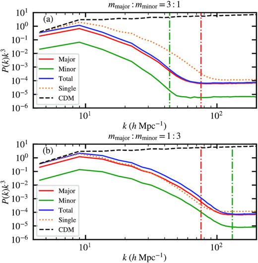
Density power spectra of the two-component model (red, green, and blue solid) at z = 10 compared to the single-component (orange dotted) and CDM (black dashed) models. Panels (a) and (b) are for mmajor: mminor = 3: 1 and 1: 3, respectively. The CDM case shares the same initial power spectrum as |$\psi \rm {DM}$| but evolves as P(k) ∝ (1 + z)−2 in the entire range of k probed here. The red and green dash-dotted vertical lines show the Jeans wavenumbers of the major and minor components at z = 10, respectively. The lowest-k mode of both the two-component total density and single component follow the CDM evolution, while larger-k modes are suppressed relative to CDM. In addition, the total density power spectrum of mmajor: mminor = 3: 1 (1: 3) is lower (higher) than that of single component due to the stronger (weaker) quantum pressure from the minor component.
Figs 2 and 3 show the projected density of the whole simulation box for mmajor: mminor = 3: 1 and 1: 3, respectively, normalized to the mean DM density of the universe ρ0. The single-component results are also shown for comparison. The large-scale structures, including both filaments and massive haloes, are very similar between the two- and single-component cases, which is expected because they share the same initial condition and the lowest-k mode is well above the Jeans scale. There are, however, fewer low-mass haloes in mmajor: mminor = 3: 1 due to the stronger quantum pressure resulting from a lighter minor component. Also note that for both mmajor: mminor = 3: 1 and 1: 3, the major-component haloes overlap well with their minor-component counterparts, suggesting that every halo in our two-component simulations is composed of both components.
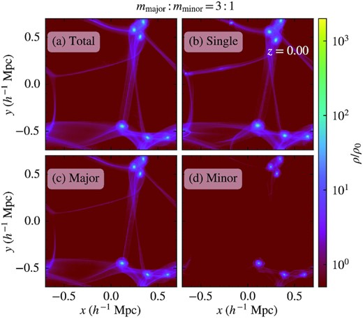
Projected density of the whole simulation box for mmajor: mminor = 3: 1 at z = 0. Panels (a), (c), and (d) show the total, major-, and minor-component densities, respectively. For comparison, we also plot the single-component result in panel (b). The spatial distribution of both filaments and massive haloes are very similar between the two- and single-component simulations, while there are fewer low-mass haloes in the two-component case due to the stronger quantum pressure resulting from the minor component. Also note that the major-component haloes overlap well with their minor-component counterparts, suggesting that every halo in our two-component simulations is composed of both components.
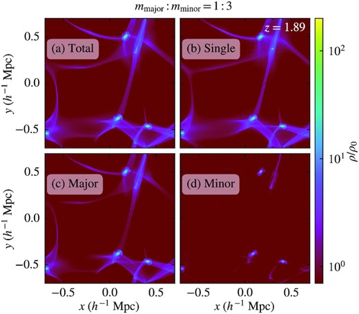
Same as Fig. 2 except that here we show the results of mmajor: mminor = 1: 3 at z = 1.89. Similar to mmajor: mminor = 3: 1, the spatial distribution of both filaments and haloes are very similar between the two- and single-component simulations and the major- and minor-component haloes overlap well with each other.
3.2 Individual haloes and solitons
We show the properties of individual haloes and solitons for the mmajor: mminor = 3: 1 simulations first followed by the mmajor: mminor = 1: 3 case.
3.2.1 mmajor: mminor = 3: 1
Here the particle masses of the major and minor components are |$m_{\rm major}=1\times 10^{-22}\, \rm eV$| and |$m_{\rm minor}=\frac{1}{3}\times 10^{-22}\, \rm eV$|, respectively. Fig. 4 shows the density distribution of a representative halo in our simulations, with a halo mass |$M_{\rm halo}\sim 2.1\times 10^{10}\, \rm {M}_{\odot }$| and a virial radius |$\sim 50\, {h^{-1}\, \rm kpc}$|. The overall structure of the two-component halo closely mimics its single-component counterpart. The wave functions outside the virial radius exhibit plane-wave features due to inflows; by contrast, the wave functions become isotropic inside the halo as a result of virialization. The wavelength is slightly shorter towards the halo centre due to the increment of velocity. In addition, the wavelength of the minor component is about three times longer than that of the major component, in agreement with mmajor: mminor = 3: 1.
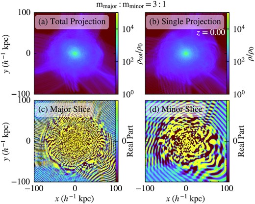
Overall structure of a representative halo in the mmajor: mminor = 3: 1 runs at z = 0. The halo mass is |$M_{\rm halo}\sim 2.1\times 10^{10}\, \rm {M}_{\odot }$| and the virial radius is |$\sim 50\, {h^{-1}\, \rm kpc}$|. Panel (a) shows the projected total density of the two-component halo, very similar to its single-component counterpart (b). Panels (c) and (d) show the real parts of the wave functions of the major and minor components, respectively, on a thin slice through the densest cell. The wave functions are plane waves outside the virial radius due to inflows and become isotropic inside the virialized halo. The wavelength of the minor component is about three times longer than that of the major component, in agreement with mmajor: mminor = 3: 1.
Fig. 5 shows the same halo in Fig. 4 but with AMR grids annotated to highlight the high resolution achieved. The mean spatial resolution within the halo is |$170\, {h^{-1}\, \rm pc}$| and the peak resolution is |$42.7\, {h^{-1}\, \rm pc}$| in the central high-density region. In comparison, the characteristic radius of the central soliton (see Fig. 7) is about several hundreds of |$\, {h^{-1}\, \rm pc}$|. Clearly, both the soliton and the density granulation throughout the halo are well resolved.
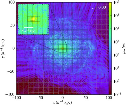
Example of the AMR grid structure. It shows the total density on a thin slice through the centre of the same halo in Fig. 4, with AMR grids annotated. Each grid represents 16 × 16 cells, with seven refinement levels, achieving maximum resolution of |$42.7\, {h^{-1}\, \rm pc}$|. The inset shows the zoomed-in view of the central high-density region of the halo. Thanks to AMR, both the central soliton (see also Figs 6 and 7) and the density granulation throughout the halo are well resolved.

Zoomed-in view of the central high-density region of the same halo in Fig. 4, showing the projected density in a slab of dimensions |$10\, {h^{-1}\, \rm kpc}\times 10\, {h^{-1}\, \rm kpc}\times 3.9\, {h^{-1}\, \rm kpc}$| centred at the soliton. We plot the total density of the two-component halo (a), the associated major-component (c) and minor-component (d) densities (so (a) = (c) + (d)), and the single-component halo (b). Solitons and density granules are manifest in both the two- and single-component haloes. In comparison to the single-component halo, in the two-component case the soliton peak density is significantly lower, the transition from soliton to halo is smoother (see also Fig. 7), and the density granules are slightly blurrier due to the presence of a longer-wavelength minor component. Solitons appear in both the major and minor components. The soliton radius and granule size of the minor component are about three times larger than that of the major component, in line with mmajor: mminor = 3: 1. The solid line in panel (c), defined as the isodensity contour where the projected minor-component density drops by half, indicates the boundary of the minor-component soliton. It shows that the major- and minor-component solitons are roughly concentric (see also Fig. 9).
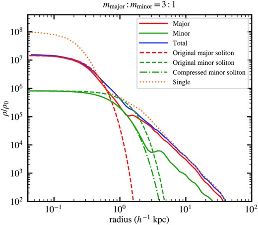
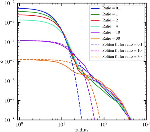
Density profiles of the same halo in Fig. 4, centred at the location of the maximum density for each case. The solid and dotted lines represent, respectively, the two- and single-component haloes, the total density profiles of which at large radii are very similar. However, the peak density of the two-component soliton is about five times lower. The dashed lines are the analytical soliton profiles, equation (4), without considering any external potential, while the dash-dotted line is the compressed soliton profile for the minor component considering the major-component soliton (red dashed line) as an external potential. As can be seen, the major-component cored profile can be well fitted by the original soliton solution, while the minor-component cored profile is better described by the compressed soliton solution. The less prominent major-component soliton together with the presence of an extended minor-component soliton lead to a much smoother soliton-to-halo transition (at |$\sim 1\, {h^{-1}\, \rm kpc}$|) in the two-component halo with mmajor: mminor = 3: 1 (see also Fig. 8).
Single-component |$\psi \rm {DM}$| haloes feature a central, dense soliton surrounded by density granules on the de Broglie scale. Fig. 6 shows a zoomed-in view of the central high-density region of the same halo in Fig. 4, demonstrating that both the soliton and density granules are still manifest in a two-component halo. However, we find several key differences between the single- and two-component cases with mmajor: mminor = 3: 1 due to the presence of a longer-wavelength minor component. The density of the two-component soliton is less dense, resulting in a smoother transition from soliton to its surrounding halo. In addition, the density granules in a two-component halo are slightly blurrier. Fig. 6 also depicts separately the density distribution of the major and minor components, showing that solitons appear in both components. The characteristic length scales of the minor-component soliton and density granules are about three times larger than that of the major component, consistent with mmajor: mminor = 3: 1. Furthermore, the major- and minor-component solitons are roughly concentric, suggesting that the soliton total density can be seen as the superposition of the individual soliton in each component. In what follows, we analyse these interesting findings in more detail.
Fig. 7 shows the radial density profiles of the same halo in Fig. 4. It confirms that the peak density of the two-component soliton is about a factor of five lower, making the solitonic structure less prominent in comparison to the single-component counterpart. On the other hand, the total density profiles at large radii are very consistent between the two cases. The major-component cored profile can be well fitted by the soliton solution (Schive et al. 2014a),
where rc is the core radius where density drops to one-half of its peak value.2 On the contrary, the minor-component cored profile cannot be well fitted by equation (4) since this component is more extended (due to a three-times lighter particle mass) and thus subject to the gravitational attraction of the interior major-component soliton. As a result, we find that the minor-component cored profile can be well fitted by a compressed soliton solution taking into account the major-component soliton as an external potential. The core radii of the major, minor, and single components are 0.25, 0.65, and |$0.18\, {h^{-1}\, \rm kpc}$|, respectively. As has been noted, the total density profile of the two-component soliton can be seen as the superposition of the individual soliton in each component with different length scales and shapes. In consequence, the less prominent major-component soliton together with the presence of an extended minor-component soliton lead to a much smoother soliton-to-halo transition in a two-component halo with mmajor: mminor = 3: 1.
Importantly, this smoother soliton-to-halo transition in the density profile will affect the associated rotation curves, as shown in Fig. 8. The ‘bump’ in the rotation velocity, an imprint of the massive and compact soliton, becomes much less prominent in the mmajor: mminor = 3: 1 halo as compared to its single-component counterpart. This new finding may have a significant impact since the predicted bump in the rotation velocity of the single-component |$\psi \rm {DM}$| scenario is in tension with observations and posing a serious challenge against |$\psi \rm {DM}$| (e.g. Bar et al. 2022).
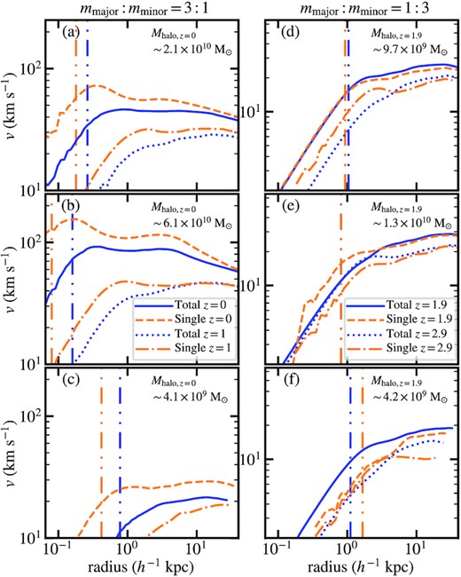
Rotation curves of the two-component haloes. Panels (a)–(c) show different haloes for mmajor: mminor = 3: 1 and panels (d)–(f) show different haloes for mmajor: mminor = 1: 3. Panels (a) and (d) are the same haloes in Figs 4 and 11, respectively. The solid blue lines represent the two-component haloes at their final redshifts (i.e. z = 0 for mmajor: mminor = 3: 1 and z = 1.89 for mmajor: mminor = 1: 3). The dashed orange lines show the single-component counterparts. The vertical dash-double-dotted lines mark the core radii of both the two- and single-component haloes at their final redshifts. The annotated Mhalo at corners of panels indicate their two-component halo masses at their final redshifts. The dotted blue and dash-dotted orange lines show the two- and single-component haloes at earlier redshifts (z = 1 for mmajor: mminor = 3: 1 and z = 2.94 for mmajor: mminor = 1: 3). The ‘bump’ in the rotation velocity, an imprint of the soliton, is less prominent in mmajor: mminor = 3: 1 due to the smoother soliton-to-halo transition (see also Fig. 7) in comparison to the single-component counterpart. In comparison, for mmajor: mminor = 1: 3, the rotation curves of the two- and single-component haloes are similar due to the absence of a minor-component soliton (see also Fig. 13). Note that the bumps in the rotation curves of panels (d)–(f) are less prominent and sometimes disappear since solitons are less stable at higher redshifts. The two-component halo at z = 1 in panel (c) is not shown because its density is too low.
Fig. 6 suggests that the major- and minor-component solitons in a mmajor: mminor = 3: 1 halo can coexist and are roughly concentric. To investigate whether it is a general feature or just a coincidence, in Fig. 9 we plot the distance between the two solitons at different redshifts. It demonstrates that the concentricity of the two solitons is a general phenomenon for mmajor: mminor = 3: 1, for which the ratio of their core radii is rc, minor/rc, major ∼ mmajor/mminor = 3 and their maximum separation is always smaller than rc, minor. This separation is likely caused by the random walk of the major-component soliton (Schive et al. 2020).
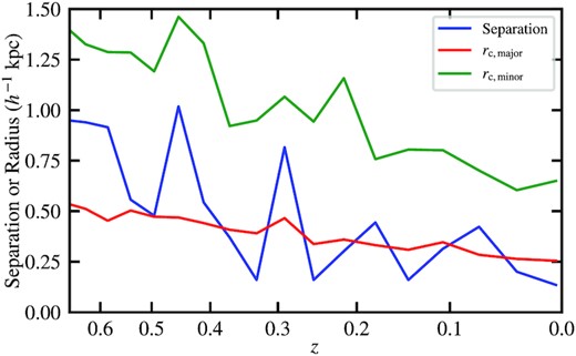
Separation distance between the major- and minor-component solitons at different redshifts for mmajor: mminor = 3: 1 (blue). For comparison, the red and green lines show the soliton core radii, rc, major and rc, minor, satisfying rc, minor/rc, major ∼ mmajor/mminor = 3. The separation distance is always smaller than rc, minor, suggesting that the two solitons move together and are roughly concentric. This separation is likely caused by the random walk of the major-component soliton (Schive et al. 2020).
Although for mmajor: mminor = 3: 1 the minor-component solitons have lower peak density in general (Fig. 7), they also have larger radii (Fig. 9). So it remains unclear whether the major- or minor-component soliton is more massive for a given halo mass, and how does that depend on the halo mass. To address this question, we show in Fig. 10 the distribution of the mass ratio between the major- and minor-component solitons in same haloes, Mc, major/Mc, minor, where the soliton mass Mc is defined as the enclosed mass within the core radius rc. It reveals that the masses of the two solitons are comparable, with ratios ranging mostly between 0.5 and 2.0 and independent of the halo mass. Note that this is a new finding different from the soliton thermodynamic expectation. Theoretically, the soliton mass is proportional to m−1 for a given halo mass (Schive et al. 2014b). With the same virial temperature, the mass ratio between the major- and minor-component solitons is expected to be 1: 3 in this case. However, the ratios we found in the simulations are ∼1: 1.
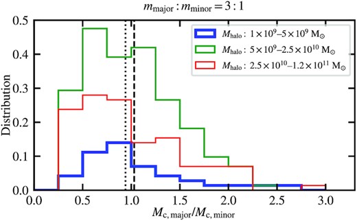
Distribution of the mass ratio between the major- and minor-component solitons in the same haloes, Mc, major/Mc, minor, for mmajor: mminor = 3: 1. We include all haloes after z < 0.63 in the three realizations and divide them into three groups by the halo mass Mhalo (blue, green, and red). The distribution is normalized such that the sum of the three areas equals unity. The dashed and the dotted vertical lines show the average and the median values of the whole distribution, respectively. The individual average and median values of each group are all within the ±4 per cent range of the vertical dashed and dotted lines, respectively. Mc, major and Mc, minor are found to be comparable, with ratios ranging mostly between 0.5 and 2.0 and independent of Mhalo.
3.2.2 mmajor: mminor = 1: 3
In this case, the particle mass of the minor component is |$m_{\rm minor}=3\times 10^{-22}\, \rm eV$|, three times larger than that of the major component, |$m_{\rm major}=1\times 10^{-22}\, \rm eV$|. The time and length scales associated with the minor component are thus three times smaller. As a result, the simulation can only reach z = 1.89 because of the much higher spatial and temporal resolutions required to properly resolve the minor component. Nevertheless, we can already identify distinct features compared to the mmajor: mminor = 3: 1 case.
Fig. 11 shows the density distribution of a representative halo with |$M_{\rm halo}\sim 9.7\times 10^{9}\, \rm {M}_{\odot }$|, corresponding to a comoving virial radius of |$\sim 47\, {h^{-1}\, \rm kpc}$|. In analogy to the mmajor: mminor = 3: 1 case shown in Fig. 4, the overall structures of the two- and single-component haloes are very similar. The wave functions exhibit plane-wave features outside the virial radius but become isotropic inside the virialized halo. The wavelength is slightly shorter towards the halo centre due to the increment of velocity. The wavelength of the minor component is about three times shorter than that of the major component, as expected from mmajor: mminor = 1: 3.
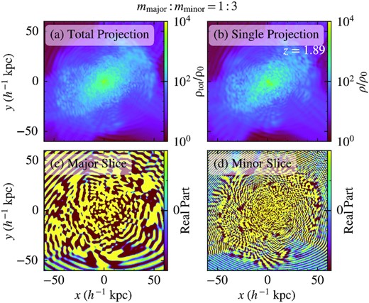
Overall structure of a representative halo in the mmajor: mminor = 1: 3 run at z = 1.89. The halo mass is |$M_{\rm halo}\sim 9.7\times 10^{9}\, \rm {M}_{\odot }$|, corresponding to a comoving virial radius of |$\sim 47\, {h^{-1}\, \rm kpc}$|. The general features of this halo are similar to the mmajor: mminor = 3: 1 case shown in Fig. 4. Panel (a) shows the projected total density of the two-component halo, very similar to its single-component counterpart (b). Panels (c) and (d) show the real parts of the wave functions of the major and minor components, respectively, on a thin slice through the densest cell. The wave functions are plane waves outside the virial radius due to inflows and become isotropic inside the virialized halo. The wavelength of the minor component is about three times shorter than that of the major component, in agreement with mmajor: mminor = 1: 3.
Fig. 12 shows a zoomed-in view of the central high-density region of Fig. 11. Both the soliton and density granulation are manifest in the total density of the two-component halo, similar to its single-component counterpart. However, surprisingly, we find that for the two-component case with mmajor: mminor = 1: 3 the soliton only forms in the major component but not in the minor component (see panel (d)). This result is distinctly different from the mmajor: mminor = 3: 1 case (e.g. see Fig. 6), where the major- and minor-component solitons can coexist and are roughly concentric. By contrast, density granulation still appears in both the major and minor components. As the images in panels (c) and (d) show, the characteristic length scale of the minor-component density granules is about three times smaller than that of the major component, consistent with the theoretical expectation of wavelength scale with the same velocity dispersion and mmajor: mminor = 1: 3. As a result, comparing panels (a) and (b) shows that the total density granulation of the two-component halo exhibits more fine structures due to the presence of a shorter-wavelength minor component.
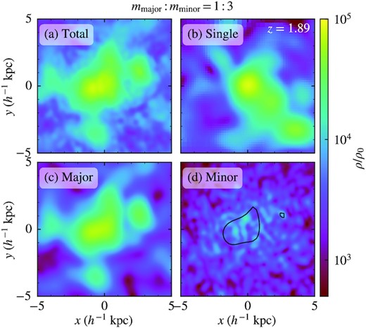
Zoomed-in view of the central high-density region of the same halo in Fig. 11, showing the projected density in a slab of dimensions |$10\, {h^{-1}\, \rm kpc}\times 10\, {h^{-1}\, \rm kpc}\times 5.98\, {h^{-1}\, \rm kpc}$| centred at the central soliton. We plot the total density of the two-component halo (a), the associated major-component (c) and minor-component (d) densities (so (a) = (c) + (d)), and the single-component halo (b). A prominent soliton can be clearly seen in the total density of both the two- and single-component haloes. However, for the former, the soliton only forms in the major component but not in the minor component. To highlight this finding, we plot in panel (d) the boundary of the major-component soliton (solid line), defined as the isodensity contour where the projected major-component density drops by half. Clearly, there is no minor-component high-density clump inside the major-component soliton. This result is distinctly different from the mmajor: mminor = 3: 1 case (e.g. see Fig. 6), where the major- and minor-component solitons can coexist and are roughly concentric. Density granulation appears in both components, the size of which is about three smaller in the minor component, consistent with mmajor: mminor = 1: 3. As a result, compared to the single-component case, the total density granulation of the two-component halo exhibits more fine structures due to the presence of a shorter-wavelength minor component.
The discovery of the absence of a minor-component soliton with mmajor: mminor = 1: 3 is important and contradictory to some previous studies (e.g. Luu et al. 2020). In the following, we provide a more detailed analysis to strengthen this finding. Fig. 13 plots the radial density profiles of the same halo in Fig. 11. It shows that the total density profiles of the two- and single-component haloes are similar at large radii, in analogy to the mmajor: mminor = 3: 1 case (see Fig. 7). However, unlike mmajor: mminor = 3: 1, here the two- and single-component cases also have a similar soliton profile on average and both exhibit a distinct soliton-to-halo transition. More importantly, it confirms that although the minor-component profile still exhibits a central density clump, it is not a soliton. Instead, this density clump is nothing but a slightly more massive granule, as suggested by the facts that (i) its density contrast is much smaller compared to a typical soliton, (ii) its peak density is only about a factor of five higher than the peak density of surrounding granules, and (iii) it is inconsistent with the soliton solution even after considering the additional compression due to the gravity of the major-component soliton (dash-dotted line). The absence of any soliton feature in panel (d) of Fig. 12 also reinforces this claim. As a result, the total density profile is dominated by the major component over the entire radius range. The corresponding rotation curves are shown in Fig. 8. The half-density radii of the major, minor, and single components are 1.00, 0.27, and |$0.93\, {h^{-1}\, \rm kpc}$|, respectively.
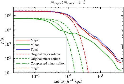
Density profiles of the same halo in Fig. 11, similar to Fig. 7 except that here is for mmajor: mminor = 1: 3. The total density profiles of the two- and single-component haloes roughly follow each other not only at large radii, but also in their central cores, which can be well fitted by the analytical soliton solution equation (4). The two-component halo virial mass is ∼15 per cent larger than the single-component halo, likely attributed to the weaker quantum pressure associated with the minor component with a higher particle mass. In contrast to the mmajor: mminor = 3: 1 case, here the single- and two-component cases have a similar soliton peak density on average and both exhibit a distinct soliton-to-halo transition. More importantly, although the minor-component profile still has a density clump at the centre, it is not a soliton because it is much lighter (also referred to Fig. 12) and cannot be well fitted by the soliton solution. See text for details.
Figs 11–13 focus on the results at the end of a mmajor: mminor = 1: 3 simulation, at which the minor-component soliton has disappeared. But what about the earlier stage? Did the minor-component soliton never form, or was it somehow disrupted at a later stage? To address this question, we plot in Fig. 14 the evolution of the peak density of the major and minor components, ρmax, major and ρmax, minor, of the same mmajor: mminor = 1: 3 halo in Fig. 11. It shows that for z ≳ 10, we have ρmax, major/ρmax, minor ∼ 3, consistent with the initial condition (see Section 2.2). Afterwards, the minor component starts to grow faster than the major component due to the weaker quantum pressure associated with the larger particle mass. The minor component collapses first at z ∼ 5, shortly after which the major component also collapses. During 5 ≳ z ≳ 3, both the major- and minor-component solitons can form but are rather unstable and get destroyed constantly and stochastically, suggesting that they are undergoing a violent relaxation process. In addition, ρmax, major and ρmax, minor are comparable and both exhibit large-amplitude oscillations during this period. After z ≲ 3, the major-component soliton becomes more stable and ρmax, major starts to grow on average again. It is at this stage that the minor-component soliton cannot re-emerge. This indicates that it is difficult for the minor-component soliton to form in a hot environment associated with the deep gravitational potential of the major-component soliton. We will discuss it in more detail in Section 4.
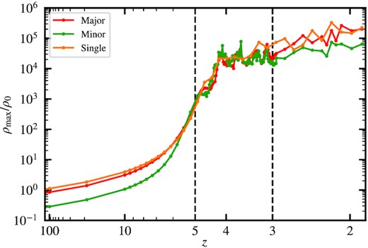
Evolution of the peak density of the major (ρmax, major; red) and minor (ρmax, minor; green) components of the same mmajor: mminor = 1: 3 halo in Fig. 11. We also plot the single-component counterpart (orange) for comparison. For z ≳ 10, we have ρmax, major/ρmax, minor ∼ 3, in accordance with the initial condition. Subsequently, the minor component grows faster due to the weaker quantum pressure and collapses at z ∼ 5. The major component also collapses shortly afterwards. Both components then go through a violent relaxation process over 5 ≳ z ≳ 3, during which both the major- and minor-component solitons form and disrupt continuously and stochastically. After z ≲ 3, the major-component soliton becomes more stable and ρmax, major starts to grow on average again; meanwhile the minor-component soliton does not re-emerge and ρmax, minor < ρmax, major thereafter. The two vertical lines mark z = 5 and 3 that roughly separate the three evolution stages mentioned above.
Fig. 15 shows the distribution of the mass ratio between the major- and minor-component solitons in the same haloes. For the comparison purpose, we still define the soliton mass Mc as the enclosed mass within the half-density radius rc even when there is no real minor-component soliton. It shows that the mass ratio is always larger than 5 and mostly exceeds ∼10, especially for massive haloes. This suggests that the minor-component solitons (or massive granules when there is no real soliton) in the mmajor: mminor = 1: 3 case have negligible effect in most cases, distinctly different from the mmajor: mminor = 3: 1 scenario (see Fig. 10). Moreover, for the minor component, the gravitational potential is mostly external and determined by the major component, and we find that the minor component is difficult to form a soliton in such an environment. See Section 4 for more discussion on this point.
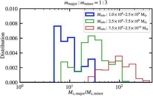
Distribution of the mass ratio between the major- and minor-component solitons in the same haloes, Mc, major/Mc, minor, for mmajor: mminor = 1: 3. We include all haloes after z < 3 in the three realizations and divide them into three groups by the halo mass Mhalo (blue, green, and red). For the comparison purpose, we define the soliton mass as the enclosed mass within the half-density radius (i.e. rc) even when there is no real minor-component soliton (see Figs 12–14 and text for the related discussion). The horizontal bins here are in log scale and the distribution is normalized such that the sum of the three areas equals unity. It shows that the mass ratio is always larger than 5 and mostly exceeds ∼10, especially for massive haloes, suggesting that the minor-component solitons have negligible effect in most cases.
4 DISCUSSION
4.1 Two-component soliton profiles
We want to obtain the minor-component soliton profile under the influence of a major-component soliton. To this end, we assume the major component still follows the original soliton solution equation (4), regard that as a static external potential, and compute the corresponding minor-component soliton solution by solving the time-independent, single-component Schrödinger–Poisson equation with spherical symmetry using the 4th order Runge–Kutta method. Additionally, since both components live at the base of the same halo potential, their velocity dispersions should be similar so the length scales should be inversely proportional to m. Therefore, we focus on the soliton solutions with a core radius ratio rc, major: rc, minor ∼ 1: 3 (3: 1) for mmajor: mminor = 3: 1 (1: 3).
Fig. 16 shows the resulting soliton density profiles. For mmajor: mminor = 3: 1, we show the minor-component solitons with a peak density ratio ρc, major/ρc, minor = 1, 4, 16, 64, and 256, corresponding respectively to a core radius ratio rc, major/rc, minor = 0.64, 0.51, 0.44, 0.41, and 0.39 and a core mass ratio Mc, major/Mc, minor = 0.27, 0.54, 1.38, 4.39, and 16.10. With a lower peak density, the minor-component soliton radius increases but the mass decreases, where rc, major/rc, minor is typically lower than 0.5 and approaching ∼0.4 while Mc, major/Mc, minor can be greater or less than unity across a wide range of peak densities. These results are consistent with our cosmological simulations, where rc, major/rc, minor ∼ 0.3–0.5 (Fig. 9) and Mc, major/Mc, minor ∼ 0.5–2.0 (Fig. 10).
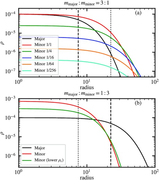
Analytical two-component soliton solutions. The black lines are the major-component solitons given by the original soliton solution equation (4). The corresponding gravitational potential is then considered as a static external potential for computing the minor-component solitons. The vertical dashed lines show the major-component soliton radius rc, major. The vertical dotted lines show 3rc, major and rc, major/3 for mmajor: mminor = 3: 1 and mmajor: mminor = 1: 3, respectively. Panel (a) shows the mmajor: mminor = 3: 1 case, where the red, green, blue, orange, and cyan lines show, respectively, the minor-component solitons with different peak density ratios, ρc, major/ρc, minor = 1, 4, 16, 64, and 256. With a lower ρc, minor, the minor-component soliton radius increases and approaches a constant ratio rc, major/rc, minor ∼ 0.4, broadly consistent with the expected value for mmajor: mminor = 3: 1 (see also Fig. 9). The mass ratio Mc, major/Mc, minor, on the other hand, can be greater or less than unity across a wide range of peak densities, in agreement with our cosmological simulations (Fig. 10). Panel (b) shows the mmajor: mminor = 1: 3 case, where we fix rc, major/rc, minor = 3 for the red line, leading to ρc, major/ρc, minor = 1/7.3 and Mc, major/Mc, minor = 3.7. The green line shows the minor-component soliton with a lower peak density, where ρc, major/ρc, minor = 1/3 and Mc, major/Mc, minor = 5.5. In comparison, the minor-component solitons in our cosmological simulations either have a relatively lower density or cannot sustain at all. See text for further discussion.
For mmajor: mminor = 1: 3, fixing rc, major: rc, minor = 3: 1 leads to ρc, major/ρc, minor = 1/7.3 and Mc, major/Mc, minor = 3.7. So the minor-component soliton appears as a small density clump on the top of the major-component soliton (which inspires the toy model presented in the next subsection). The mass ratio will increase further with a larger ρc, major/ρc, minor. For example, for ρc, major/ρc, minor = 1/3, Mc, major/Mc, minor increases to 5.5. In comparison, in our cosmological simulations the minor-component soliton (i) has a peak density generally lower than 7.3ρc, major during the violent relaxation phase (5 ≳ z ≳ 3 in Fig. 14) and (ii) does not re-emerge once the major-component soliton is stabilized (z ≲ 3). It suggests that a minor-component soliton with mmajor: mminor = 1: 3 is unstable and difficult to form in a hot environment caused by the deep gravitational potential of the major-component soliton. We discuss it further in the next subsection.
4.2 Toy model for minor-component soliton formation
Here we propose a toy model to investigate why a minor-component soliton cannot re-emerge with the presence of a stable major-component soliton for mmajor: mminor = 1: 3 (Figs 12–15). We let 10 minor-component solitons merge in a static simple harmonic potential, Φ(r) ∝ r2, mimicking a major-component soliton. All solitons are initially at rest and randomly distributed. We experiment with different depths of the simple harmonic potential, using the energy ratio between the simple harmonic potential energy and the self-gravitational potential energy of all solitons in the initial conditions as an indicator, and compare the final relaxed configurations after merger. The simulations are dimensionless.
Figs 17 and 18 show, respectively, the projected density and density profiles of the final states with different initial energy ratios. When the simple harmonic potential is deeper, the environment is hotter, and the central object formed after merger becomes more diffusive and less prominent. As the energy ratio exceeds ∼10, the density profiles start to deviate from the soliton solution and the soliton does not form during the entire merging and relaxation process. It indicates that it is difficult to form a soliton in a hot environment under a deep potential, consistent with our cosmological simulations. For mmajor: mminor = 1: 3, the gravitational potential near the halo centre is dominated by the massive major-component soliton, which serves as an external hot environment that hinders the formation of a minor-component soliton. Here the hot environment simply means the gravitational potential is deep.
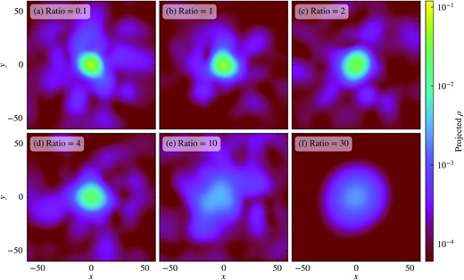
Projected density in the toy model described in Section 4.2, with 10 minor-component solitons merging in a static simple harmonic potential mimicking a major-component soliton. This figure shows the final relaxed state for investigating whether a single soliton can re-emerge after merger. Different panels show the simulations with different energy ratios between the simple harmonic potential energy and the self-gravitational potential energy of all solitons in the initial conditions. As the energy ratio increases (i.e. a deeper simple harmonic potential), the central object in the final state becomes more diffusive and deviates from the soliton solution (see Fig. 18), especially when the energy ratio exceeds ∼10 (panels (e) and (f)). Not only the soliton cannot form at the end, but it never forms during the entire merging and relaxation process when the energy ratio is large. It indicates that a soliton is difficult to form in a hot environment under a deep potential. This toy model provides a plausible explanation for why a minor-component soliton cannot form for mmajor: mminor = 1: 3 (Figs 12–15).
Density profiles of the six systems in Fig. 17 (solid lines). The dashed lines represent the fitted analytical soliton solutions considering the simple harmonic external potential for comparison. The larger the energy ratio, the lower the peak density and mass of the central object after merger. Especially, the density profiles start to deviate from the soliton solution when the energy ratio exceeds ∼10, suggesting that a soliton is difficult to form in a hot environment under a deep potential, consistent with our cosmological simulations with mmajor: mminor = 1: 3 (Figs 12–15).
The above finding has some intriguing implications. For example, Luu et al. (2020) suggest that the nuclear star cluster of the Milky Way can be explained by nested solitons from two |$\psi \rm {DM}$| components, with |$m_{\rm major}\sim 10^{-22}\, \rm eV$| and |$m_{\rm minor}\sim 10^{-20}\, \rm eV$|. However, if our results could be extrapolated to a higher particle mass ratio and different DM density fraction, it would imply that such a higher-particle-mass minor-component soliton cannot form. Another important question concerns whether a single-component soliton can form under the deep gravitational potential of a baryonic bulge with mass |$\sim 10^{10} \, \rm {M}_{\odot }$|, an order of magnitude more massive than a typical soliton in a Milky Way-sized halo. If it cannot form, the conventional core–halo relation (e.g. Schive et al. 2014b) must take into account this diversity.
4.3 Two-component core–halo relation
A natural follow-up question is whether there is a relation between the two-component solitons and their host haloes. For mmajor: mminor = 1: 3, the minor-component core is negligible (Fig. 15), while the major-component soliton is similar to its single-component counterpart (Fig. 13). So the major component (or the sum of both components since the minor-component core mass is negligible anyway) should follow the same single-component core–halo mass relation, |$M_{\rm c} \propto M_{\rm halo}^{1/3}$| (Schive et al. 2014b). But what about mmajor: mminor = 3: 1, for which the major- and minor-component soliton masses are comparable (Fig. 10)?
Fig. 19 shows Mc versus Mhalo for mmajor: mminor = 3: 1 and the single-component case. Even considering the scatter in the data points, both the major- and minor-component soliton masses are clearly lower than their single-component counterpart, consistent with Fig. 7. However, to our surprise, the combined soliton mass of the two components, Mc, combined = Mc, major + Mc, minor, is generally similar to the single-component soliton mass. It suggests that there is a more general core–halo relation where the soliton mass in the original single-component core–halo relation can be replaced by the combined soliton mass of two components (for both mmajor: mminor = 3: 1 and 1: 3). This is also a new finding to show the soliton thermodynamics has a serious problem when extended to multi-component cases. The soliton mass is expected to be an extensive quantity in soliton thermodynamics since it is mainly controlled by the virial temperature in the halo (even though there may be small scatter in the relation). If we have N components, the total soliton mass will be |$\sum _{{\rm n}=1}^{\rm N} M_{\rm c,n}$|, which is much bigger than the single-component soliton mass for a given halo mass. This is, however, not the case in our simulation result. On the contrary, our result seems to indicate the soliton mass is an intensive quantity in the thermodynamic sense. This problem and the soliton mass ratio problem (Fig. 10) both indicate the original single-component soliton thermodynamics fails.
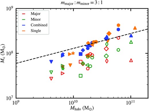
Core–halo mass relation at z = 0 for mmajor: mminor = 3: 1. The same halo of different components is represented by the same symbol with different colours. Even considering the scatter in the data points, both the major-component (red) and minor-component (green) soliton masses are clearly lower than their single-component counterpart (orange), consistent with Fig. 7. However, the combined soliton mass of the two components (blue) is generally similar to the single-component soliton, suggesting that the combined mass in a mmajor: mminor = 3: 1 system follows the original single-component core–halo mass relation, |$M_{\rm c} \propto M_{\rm halo}^{1/3}$| (dashed line).
Furthermore, we propose that the soliton mass of individual component (Mc, major or Mc, minor) is proportional to its initial mass density fraction (75 and 25 per cent for the major and minor components, respectively) and inversely proportional to the DM particle mass (mmajor or mminor). This conjecture leads to Mc, major: Mc, minor = 1: 1 for mmajor: mminor = 3: 1 and Mc, major: Mc, minor = 10: 1 for mmajor: mminor = 1: 3, qualitatively consistent with our cosmological simulations.
However, we emphasize that, unlike the single-component case, the above two-component core–halo relation is purely empirical and requires further investigation and justification in the future.
4.4 Minor-component power spectrum
The addition of a minor component can reshape the total |$\psi \rm {DM}$| density power spectrum (Fig. 1), which may help alleviate some existing tension between theories and observations. For example, the power spectrum of mmajor: mminor = 1: 3 at z = 10 is noticeably higher than the single-component case at high k. This enhanced small-structure power in filaments at high redshifts may diminish the tension between Lyman-α forest observations and |$\psi \rm {DM}$| predictions (e.g. Iršič et al. 2017), although a variation of |$\psi \rm {DM}$|, the extreme-axion model, is also able to alleviate the inconsistency (Zhang & Chiueh 2017a, b; Leong et al. 2019). On the other hand, the power spectrum of mmajor: mminor = 3: 1 grows slower than the single-component case at high k. If our results are extrapolated to a higher particle mass ratio case (e.g. mmajor: mminor = 15: 1), it may provide a possible solution to the σ8 tension (e.g. Abdalla et al. 2022) that the observed matter fluctuations smoothed over |$8 \, {h^{-1}\, \rm Mpc}$| are smaller than the ΛCDM prediction.
5 CONCLUSION
In this work, we explore a two-component |$\psi \rm {DM}$| scenario via cosmological simulations. The two components are described by two separate scalar fields coupled only by gravity, and their evolution is governed by the coupled Schrödinger–Poisson equations (1)–(3). By utilizing the AMR code |$\small {GAMER-2}$| to achieve sufficient high resolution (Fig. 5), we focus on the non-linear structures of two-component haloes and solitons in a |$1.4 \, {h^{-1}\, \rm Mpc}$| comoving box. We assume the total dark matter mass contains 75 per cent major component and 25 per cent minor component, fix the major-component particle mass to |$m_{\rm major}=1\times 10^{-22}\, \rm eV$|, and explore two different minor-component particle masses, mmajor: mminor = 3: 1 and 1: 3. Our main results are summarized as follows:
On large scales, the spatial distributions of filaments and massive haloes are very similar between the two- and single-component models (Figs 2 and 3).
For both mmajor: mminor = 3: 1 and 1: 3, haloes are composed of both components, and each of which exhibits distinct wave features (e.g. density granulation) with a characteristic length scale inversely proportional to the particle mass m (Figs 4 and 11). The outskirts of the two-component halo density profile closely follow the single-component counterpart (Figs 7 and 13).
In mmajor: mminor = 3: 1 haloes, major- and minor-component solitons coexist and are roughly concentric (Figs 6 and 9). The major-component soliton follows the original soliton profile (equation 4) while the minor-component soliton follows a compressed soliton profile (Fig. 16); both components contribute comparably to the soliton total density profile. The soliton peak density is significantly lower than the single-component counterpart, which, together with the presence of an extended minor-component soliton, leads to a much smoother soliton-to-halo transition (Fig. 7). As a result, the bump in the rotation velocity stemming from a massive and compact single-component soliton becomes much less prominent in a mmajor: mminor = 3: 1 halo (Fig. 8), which can alleviate the tension with some observations (e.g. Bar et al. 2022).
In mmajor: mminor = 3: 1 haloes, the masses of the major- and minor-component solitons are comparable, with ratios ranging mostly between 0.5 and 2.0 and independent of halo mass (Fig. 10). This result is consistent with the two-component soliton solutions (Fig. 16). The combined mass of the major- and minor-component solitons is found to follow the original single-component core–halo mass relation, |$M_{\rm c, combined} = M_{\rm c, major}+ M_{\rm c, minor}\propto M_{\rm halo}^{1/3}$| (Fig. 19). These results indicate the single-component soliton thermodynamic expectation fails to extend to the multi-component cases.
In mmajor: mminor = 1: 3 haloes, the minor-component soliton cannot form once the major-component soliton is stabilized (Figs 12–15). This surprising result can be explained by the toy model in Section 4.2, showing that a soliton cannot re-emerge after falling in a deep simple harmonic potential (Figs 17 and 18). It suggests that it is difficult to form a soliton in a hot environment associated with a deep potential. The total density profile in mmajor: mminor = 1: 3, for both halo and soliton, is thus dominated by the major component and closely follows the single-component profile (Fig. 13).
The above findings provide a set of predictions that sheds light on a multi-component |$\psi \rm {DM}$| model. For future work, we can explore different particle mass ratios and different total mass ratios. What is the critical ratio to show a significant difference compared with the single-component scenario? Would a minor component with a much larger particle mass (e.g. mmajor: mminor = 1: 10) collapse earlier and form stable solitons? What happens if there are more than two components or even a continuous distribution of different particle masses? Last but not least, we want to explore whether a massive bulge can provide a hot environment to disrupt the soliton even in the single-component scenario.
ACKNOWLEDGEMENTS
We thank to National Center for High-performance Computing (NCHC) for providing computational and storage resources. HS acknowledges funding support from the Jade Mountain Young Scholar Award No. NTU-111V1201-5, sponsored by the Ministry of Education, Taiwan. This research is partially supported by the National Science and Technology Council (NSTC) of Taiwan under Grants No. NSTC 111-2628-M-002-005-MY4, No. NSTC 108-2112-M-002-023-MY3, and No. NSTC-110-2112-M-002-018, and the NTU Academic Research-Career Development Project under Grant No. NTU-CDP-111L7779.
DATA AVAILABILITY
The data underlying this article will be shared on reasonable request to the corresponding author.
Footnotes
Throughout this paper, we use the term ‘core radius rc’ to refer to the radius where the shell-average density in the simulation data is one-half of the peak density, but not the core radius derived from the fitted original or compressed soliton solution.
References
APPENDIX A: CODE VERIFICATION
To verify the accuracy of our cosmological two-component |$\psi \rm {DM}$| code, we conduct the following two numerical tests: two-component Jeans instability test (Section A1) and two-component solitons test (Section A2).
A1 Two-component Jeans instability test
We review the single-component |$\psi \rm {DM}$| Jeans instability in Section A1.1, generalize it to two components in Section A1.2 and conduct numerical experiments in Section A1.3.
A1.1 Single-component Jeans instability
Assume the background density of the universe is ρbg. The overdensity is defined as
where |$\Delta \rho (\boldsymbol{x})$| is the density perturbation with the total density given by |$\rho (\boldsymbol{x})=\rho _{\rm bg}+\Delta \rho (\boldsymbol{x})$|. After Fourier transformation, |$\delta (\boldsymbol{x})$| can be decomposed into different k modes. For simplicity, we only keep the cosine terms,
By introducing
where a is the scale factor of cosmic expansion, m is the |$\psi \rm {DM}$| particle mass, H0 is the current Hubble parameter, and
is the Jeans wavenumber, the linearized equation for the evolution of wave dark matter overdensity can be written as (Woo & Chiueh 2009)
The general solution to equation (A5) is
where c+ and c− are the coefficients of the growing and decaying modes, respectively. Given a fixed k, y decreases when a increases.
The critical wavenumber k = kJ corresponds to |$y=y_{\rm J}=\sqrt{6}$|. On small scales with k > kJ (y > yJ), perturbations are stable and oscillating since quantum pressure balances gravity. In the limit y ≫ 1, the solution equation (A6) reduces to
In contrast, on large scales with k < kJ (y < yJ), perturbations are unstable and can collapse since gravity dominates over quantum pressure, known as the Jeans instability. For y ≪ 1, the solution equation (A6) reduces to
where the growing mode evolves as δk ∝ y−2 ∝ a, same as CDM.
Assume the wave function takes the form ψ = Rbg + ΔR + iΔI, where R and I are the real and imaginary parts, respectively. The corresponding linearized solution of the wave function perturbations ΔR and ΔI can be derived in a similar way (Woo & Chiueh 2009). The perturbation of real part Rk follows the same equation as the density perturbation equation (A5). The perturbation of imaginary part satisfies Ik = −dRk/dy. For a single-mode perturbation, the real part of the wave function is
the imaginary part is
and the density is
Note that the linearization assumes |$I_k^2 \ll 2R_k \ll R_{\rm bg}$|.
A1.2 Two-component Jeans instability
Here we extend the original single-component Jeans instability to two components. The background density fractions of components 1 and 2 are given, respectively, by f1 = ρbg, 1/ρbg and f2 = ρbg, 2/ρbg, where 0 ≤ f1 ≤ 1, 0 ≤ f2 ≤ 1, and f1 + f2 = 1. The density distribution of each component can be written as
where |$\Delta \rho _1(\boldsymbol{x})$| and |$\Delta \rho _2(\boldsymbol{x})$| are the perturbations of individual components, corresponding to overdensities
The total overdensity is then given by
After Fourier transformation, individual overdensity can be decomposed into different k modes
where for simplicity we only keep the cosine terms and assume the two-component perturbations are in phase. The Jeans wavenumber of each component is
where m1 and m2 are the respective particle masses. Similar to equation (A3), we define y1 and y2 as
The two-component linearized equations coupled through a common gravity read
Here we use the same y in the single-component case (equation A3) as the independent variable and keep the single-component m as a reference particle mass in order to write the equations in a more symmetric form.
We do not find an exact solution to equation (A18). However, an approximate solution can be obtained under the small-scale or large-scale limit. In the small-scale limit with |$\frac{m}{m_1}y\gg 1$| and |$\frac{m}{m_2}y\gg 1$|, the two components become decoupled and equation (A18) reduces to
The solutions to equation (A18) are
where c1, c2, c3 and c4 are coefficients determined by the initial conditions. In this limit, both components are stable and oscillating with their own frequency, similar to equation (A7).
In the large-scale limit with |$\frac{m}{m_1}y\ll 1$| and |$\frac{m}{m_2}y\ll 1$|, equation (A18) reduces to
The solutions to equation (A21) are
where c5, c6, c7, and c8 are coefficients determined by the initial conditions. There are two extra terms in this solution compared to equation (A8). In this limit, both components are unstable.
Similar to the single-component case equations (A9)–(A11), we can express the linearized solutions of the two-component wave functions explicitly as the component-1 real part
the component-1 imaginary part
the component-1 density
the component-2 real part
the component-2 imaginary part
and the component-2 density
The linearization is valid when |$I_{k,1}^2\ll 2R_{k,1}\ll R_{\rm bg,1}$| and |$I_{k,2}^2\ll 2 R_{k,2}\ll R_{\rm bg,2}$|.
A1.3 Numerical tests
We utilize the aforementioned two-component Jeans instability problem to verify the cosmological code used in this work. We test both the stable and unstable solutions, which share the following set-up. The matter density parameter is Ωm = 1.0 and the dimensionless Hubble parameter is h = 0.6732. We assume a single-mode perturbation with a wavevector |$\boldsymbol{k}=(k/\sqrt{3},k/\sqrt{3},k/\sqrt{3})$| along the diagonal of the computational domain. The perturbation wavelength is |$\lambda =L/\sqrt{3}$|, where L is the comoving box size, such that there are three waves along the diagonal. The two components share the same wavevector and are in phase. To mimic our cosmological simulations, we adopt |$m_1=1\times 10^{-22}\, \rm eV$|, |$m_2=\frac{1}{3}\times 10^{-22}\, \rm eV$|, f1 = 0.75, and f2 = 0.25. The reference particle mass in equation (A17) is |$m=1\times 10^{-22}\, \rm eV$|.
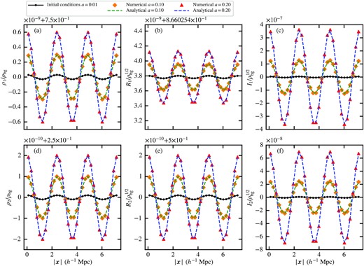
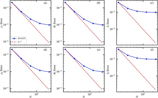
First, we test the stable case. The analytical solutions are given by equations (A20), (A23)–(A28), where the coefficients are set to c1 = −3.0 × 10⁻⁵, c2 = 0, c3 = −3.0 × 10⁻⁵, c4 = 0 and the perturbation amplitudes are |$R_{k,1}= 1.09\times 10^{-6}\sqrt{\rho _{\rm bg}}$|, |$I_{k,1}= 1.29\times 10^{-5}\sqrt{\rho _{\rm bg}}$|, |$R_{k,2}= -1.79\times 10^{-6}\sqrt{\rho _{\rm bg}}$|, and |$I_{k,2}= -7.28\times 10^{-6}\sqrt{\rho _{\rm bg}}$|. The comoving box size is |$L=0.0042\, {h^{-1}\, \rm Mpc}$|, corresponding to a wavenumber |$k=2591.14\, {h\, \rm Mpc^{-1}}$|. We evolve the system from a = 0.0005 to 0.00050018 such that component 1 oscillates for ∼1.1 periods. During this time span, y1 evolves from 3.8753 × 10⁴ to 3.8746 × 10⁴ and y2 evolves from 1.16259 × 10⁵ to 1.16238 × 10⁵. The initial Jeans wavenumbers are |$k_{\rm J,1}= 20.60\, {h\, \rm Mpc^{-1}}$| and |$k_{\rm J,2}= 11.89\, {h\, \rm Mpc^{-1}}$|, satisfying k ≫ kJ, 1 and k ≫ kJ, 2. Fig. A1 compares between the simulation results with N3 = 323 cells and analytical solutions, demonstrating good agreement. Fig. A2 shows the error convergence with different N. Here we define the error as
where ‘|$\rm i$|’ is the cell index along the diagonal, ‘|$\rm Numerical_i$|’ is the simulation data, ‘|$\rm Analytical_i$|’ is the analytical solution and ‘|$\rm Analytical_{\rm bg}$|’ represents the background term. It shows that the numerical accuracy is better than second-order in this test.
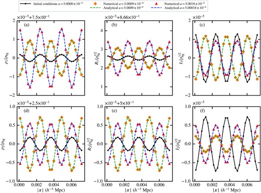
Two-component Jeans instability test: stable case. Panels (a)–(c) show respectively the density, real part, imaginary part of component 1 and panels (d)–(f) show the results of component 2. Diamonds and triangles show the numerical results at two different redshifts. Dashed lines represent the corresponding analytical solutions (equations (A20), (A23)–(A28)). Black solid lines with dots give the initial conditions for reference. The simulation set-up is described in Section A1.3. Perturbations are oscillating in this case. The simulation end time a = 0.00050018 corresponds to ∼1.1 oscillation periods for component 1 and more than three periods for component 2. The numerical results agree well with the analytical solutions.
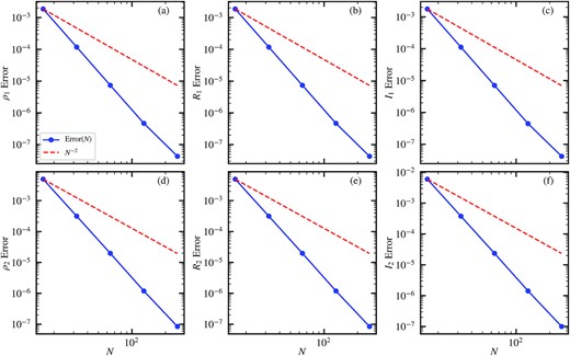
Error convergence in the two-component Jeans instability test: stable case. Panels (a)–(c) show respectively the errors of density, real part, and imaginary part of component 1 and panels (d)–(f) show the errors of component 2. Blue solid lines with dots show the simulation results, which are better than second-order accuracy (red dashed lines) in this test.
Second, we test the unstable case. The analytical solutions are given by equations (A22)–(A28), where the coefficients are set to c5 = 3.0 × 10⁻¹⁵, c6 = 0, c7 = 0, and c8 = 0 to keep only the growing mode. The initial perturbation amplitudes are |$R_{k,1}=1.73\times 10^{-11}\sqrt{\rho _{\rm bg}}$|, |$I_{k,1}=3.99\times 10^{-9}\sqrt{\rho _{\rm bg}}$|, |$R_{k,2}=9.99\times 10^{-12}\sqrt{\rho _{\rm bg}}$|, and |$I_{k,2}=7.68\times 10^{-10}\sqrt{\rho _{\rm bg}}$|. The comoving box size is |$L=4.2\, {h^{-1}\, \rm Mpc}$|, corresponding to a wavenumber |$k=2.59\, {h\, \rm Mpc^{-1}}$|. We evolve the system from a = 0.01 to 0.2 such that the density perturbation amplitudes of both components will grow by a factor of 20. During this time span, y1 evolves from 8.67 × 10⁻³ to 1.94 × 10⁻³ and y2 evolves from 2.60 × 10⁻² to 5.81 × 10⁻³. The initial Jeans wavenumbers are |$k_{\rm J,1}= 43.56\, {h\, \rm Mpc^{-1}}$| and |$k_{\rm J,2}= 25.15\, {h\, \rm Mpc^{-1}}$|, obeying k ≪ kJ, 1 and k ≪ kJ, 2. Fig. A3 demonstrates good agreement between the simulation results with N3 = 323 cells and analytical solutions. Fig. A4 shows the error convergence with different N. It is roughly second-order at lower resolution for the densities and real parts of both components. But at higher resolution, especially for the imaginary parts, errors converge much slower than second-order, possibly due to linearization errors or round-off errors.
Similar to Fig. A1 but for the unstable case. The analytical solutions are given in equations (A22)–(A28). Perturbations are unstable and growing linearly with a. The simulation end time a = 0.2 corresponds to when the density perturbation amplitude has grown by a factor of 20. The numerical results match well with the analytical solutions.
Similar to Fig. A2 but for the unstable case. The error convergence is roughly second-order at lower resolution for the densities and real parts of both components. But at higher resolution, especially for the imaginary parts, errors converge much slower than second-order, possibly due to linearization errors or round-off errors.
A2 Two-component solitons test
To further validate our two-component |$\psi \rm {DM}$| code in the fully non-linear regime, we test the stability of two concentric solitons with distinct particle masses via three-dimensional simulations. We adopt mmajor: mminor = 3: 1 and ρc, major/ρc, minor = 64. The compressed minor-component soliton is taken to be the same as the orange line in Fig. 16 that considers the original (uncompressed) major-component soliton (equation 4) as an external potential. To improve consistency, for the major-component soliton, we further consider the additional compression due to the external potential associated with the minor-component soliton. Ideally, to be fully self-consistent, one should repeat this iterative procedure until both soliton solutions converge. However, it only has a small effect since the compact and massive major-component soliton is insensitive to the minor-component potential. So we do not apply this iterative method here.
We adopt a non-comoving box with a rigid wall boundary condition. The simulation box has a size of L ∼ 72rc, major. The base level resolution is N = 128 and there are three refined AMR levels, leading to ∼14 cells for resolving rc, major. Fig. A5 shows the simulation results. We confirm that both solitons remain stable after the major- and minor-component soliton wave functions undergo 8 and 1 oscillations, respectively. There is a ∼10 per cent fluctuation in the peak density of the major-component soliton, likely because the two-component solitons are not constructed fully self-consistently as mentioned above. This test confirms the accuracy of (i) the compressed soliton solutions and (ii) our two-component |$\psi \rm {DM}$| code.
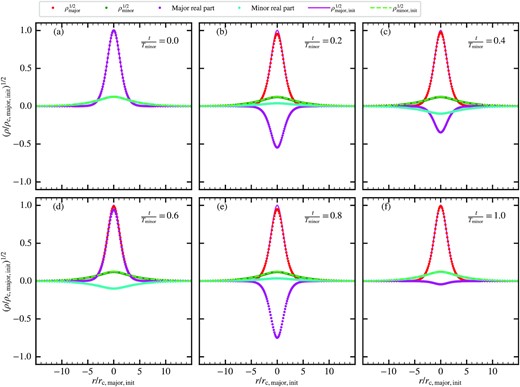
Evolution of two concentric solitons with distinct particle masses. Panels (a)–(f) show the data along the diagonal of the box at different time, where Tminor is the oscillation period of the minor-component soliton wave function. Red and green dots show respectively the square root of the major- and minor-component density, and magenta solid and lime dashed lines show the initial conditions for comparison. Purple and cyan dots are the real parts of the major- and minor-component wave functions, respectively. It is expected that the soliton density is almost stationary but the wave function is oscillating for both components. At the simulation end time, the major-component (minor-component) soliton wave function undergoes 8 (1) oscillations. We find that both solitons are stable, confirming the accuracy of the two-component |$\psi \rm {DM}$| code used in this work. There is a ∼10 per cent fluctuation in the peak density of the major-component soliton, likely because the two-component solitons are not constructed fully self-consistently (see text for details).
