


ABSTRACT
We performed a detailed broad-band spectral and timing analysis of a small flaring event of ∼120 ks in the narrow-line Seyfert 1 galaxy NGC 4051 using simultaneous XMM–Newton and NuSTAR observations. The ∼300 ks long NuSTAR observation and the overlapping XMM–Newton exposure were segregated into pre-flare, flare, and post-flare segments. During the flare, the NuSTAR count rate peaked at 2.5 times the mean count rate before the flare. Using various physical and phenomenological models, we examined the 0.3–50 keV X-ray spectrum, which consists of a primary continuum, reprocessed emission, warm absorber and ultrafast outflows at different time-scales. The mass of the central black hole is estimated to be ≥1.32 × 10⁵ M⊙ from spectral analysis. The absence of correlation between the flux in the 6–7 keV and 10–50 keV bands suggests different origins of the iron emission line and the Compton hump. From the spectral analysis, we found that the reflection fraction drops significantly during the flare, accompanied by an increase in the coronal height above the disc. The spectrum became soft during the flare, supporting the ‘softer when brighter’ nature of the source. After the alleviation of the flare, the coronal height drops and the corona heats up. This indicates that there could be inflation of the corona during the flare. We found no significant change in the inner accretion disc or the seed photon temperature. These results suggest that the flaring event occurred due to a change in coronal properties rather than any notable change in the accretion disc.
1 INTRODUCTION
Active galactic nuclei (AGNs) are accreting supermassive black holes (SMBHs) of mass > 105 M⊙, located at the centre of almost every galaxy. These are considered to be powerful sources (luminosities up to 1048 erg s−1) in the Universe, which emit in the entire range of the electromagnetic spectrum. Ultraviolet/optical photons originating from a thermal accretion disc are inverse-Comptonized in the hot corona of relativistic electrons near the black hole and produce X-ray continuum emission (Haardt & Maraschi 1993), which can be approximated by a power law with an exponential cut-off. However, the origin of the compact corona and its nature, structure, and location are still unknown. Recent studies put forward the hint of a connection between the corona and the jet (Zhu et al. 2020). It is hypothesized that, in Seyfert galaxies (or radio-quiet AGNs), the corona may be powered by magnetic flux tubes associated with the accretion disc near the black hole. These flux tubes get inflated due to the differential rotation of the black hole and the accretion disc, and strong confinement from the surrounding medium quenches the launching of jets. As a result, the plasma gets heated up and produces X-ray emission (Yuan et al. 2019). This X-ray emission shows high variability in timing and spectral properties on short as well as long time-scales (Kumari et al. 2021). Rapid and small variability, where the count rate in different energy ranges changes by a factor of two or three, is frequently observed in AGNs and is attributed primarily to the change in coronal topology.
Narrow-line Seyfert galaxies of type 1 (NLS1s) are a subcategory of AGNs and are believed to be accreting mass at a high rate, close to the Eddington limit (Komossa et al. 2006). In the X-ray band, NLS1s show a steep X-ray spectral slope (Γ ∼ 1.6–2.5; Vaughan et al. 1999). It is proposed that when the accretion rate is high more soft photons are produced, causing the corona to cool down rapidly and produce brighter and softer spectra (Shemmer et al. 2008). NLS1s are known to show strong reprocessed emission, a soft excess below 2 keV, and signatures of ionized or neutral absorbers (Wang, Brinkmann & Bergeron 1996; Fabian et al. 2002) in their spectra. Moreover, strong outflows have been observed in these objects, which are associated with a high mass accretion rate (Laha et al. 2021). NLS1s are well known to show strong soft X-ray excess below 2 keV, though the origin of this feature is still debatable. There are different models to explain the origin of this component, e.g. warm Comptonization in relatively cool and optically thick plasma (Done et al. 2012; Kubota & Done 2018) and relativistic blurred reflection from the inner disc (Fabian et al. 2004). Some authors also suggest that fewer scatterings in the corona, which can generate higher variability than a large number of scatterings, could also possibly lead to the origin of the soft excess (Nandi et al. 2021).
NGC 4051, a nearby (z = 0.00234) galaxy, is one of the brightest NLS1 galaxies with a mass ∼1.7 × 10⁶ M⊙ (Denney et al. 2009). It is a low-luminosity (∼1041 erg s−1) NLS1 galaxy, which shows rapid flux and spectral variability (e.g. Guainazzi et al. 1996) on different time-scales and a number of emission/absorption features in the spectrum. The X-ray spectral and timing variabilities of this AGN have been studied copiously in the past. Using 1000 days of data from 1996–1999, Lamer et al. (2003) reported a very hard spectrum during its low state. There was underlying reflection emission, likely from the molecular torus, in all flux states. They found an anti-correlation between the X-ray flux and the spectral hardness. Similar results have been reported by Pounds et al. (2004), where the reflection of hard X-rays from cold matter was found along with a non-variable and narrow iron Kα fluorescent line. The difference between the low and high flux spectral states was interpreted in terms of varying properties of the outflowing gas. Ponti et al. (2006) studied time-resolved spectra using XMM–Newton observations and calculated the slope–flux correlation in the low and high flux states. Mizumoto & Ebisawa (2016) found the presence of different kinds of warm absorbers (WAs) in the X-ray spectrum and their variability. Seifina, Chekhtman & Titarchuk (2018) reported a correlation between the X-ray spectral photon index and the mass accretion rate using XMM–Newton, Suzaku, and RXTE observations. This provided an estimate of the lower limit of the black hole mass in NGC 4051 as 6 × 10⁵ M⊙. In this work, we report the results from the X-ray timing and spectral analysis of simultaneous XMM–Newton and NuSTAR observations of NGC 4051 in 2018 November. We investigated the spectral variability in three time intervals of the observations to examine the changes in the X-ray-emitting corona with flux variability.
This work is organized as follows. Section 2 describes the observations of NGC 4051 with the XMM–Newton and NuSTAR observatories and the corresponding data reduction processes. The results from a time-resolved spectral analysis and timing analysis are discussed in Section 3. The implications of the results have been discussed in Section 4. Finally, the conclusions have been summarized in Section 5. In this work, we used the cosmological parameters H0 = 70 km s−1 Mpc−1, Λ0 = 70, and σM = 0.27.
2 OBSERVATIONS AND DATA REDUCTION
NGC 4051 was observed with NuSTAR (Harrison et al. 2013) and XMM–Newton(Jansen et al. 2001) multiple times during the last two decades. Most recently, it was observed with NuSTAR in 2018 November simultaneously with XMM–Newton. The observation details are given in Table 1. Two observation IDs of XMM–Newton that are used in this work were studied by Wu et al. (2020).
Log of 2018 November simultaneous observations of NGC 4051 with NuSTAR and XMM–Newton. The quoted count rate for NuSTAR observations is the average count rate over the entire observation period.
| ut date (start) | ut date (end) | NuSTAR | Total exp (ks) | Count s−1 | XMM–Newton | Exp (ks) | Count s−1 |
|---|---|---|---|---|---|---|---|
| 2018-11-04 12:56:09 | 2018-11-11 14:46:09 | 60 401 009 002 | 311.1 | 0.45 | – | – | – |
| 2018-11-07 09:59:39 | 2018-11-08 10:26:15 | – | – | – | 0 830 430 201 | 83.2 | 13.84 |
| 2018-11-09 09:48:58 | 2018-11-10 09:02:59 | – | – | – | 0 830 430 801 | 85.5 | 8.59 |
XMM–Newton
In this work, we used European Photon Imaging Camera (EPIC)-pn (Strüder et al. 2001) small window mode data, due to their higher sensitivity. We reprocessed the EPIC-pn data using the standard System Analysis Software (SAS v.19.1.0: Gabriel et al. 2004) and updated calibration files. To check for the presence of any flaring particle background, we generated a light curve above 10 keV. We created good time interval (GTI) files by excluding the time intervals containing particle background, which were capped by the count rate. We used <0.15 and <0.2 count s−1 for Obs. IDs 0 830 430 801 and 0 830 430 201, respectively. This resulted in corresponding net exposures of ∼73.8 and ∼68.8 ks. We considered events with PATTERN ≤ 4 for EPIC-pn. We also checked for the photon pile-up effect using the epatplot task. We extracted source and background spectra by selecting circular regions of 30-arcsec radii for both observations. We generated light curves in different energy bands using the xselect task of FTOOLS. The redistribution matrix and ancillary response files were generated by the arfgen and rmfgen tasks, respectively. We grouped the spectral data sets to a minimum of 30 counts per bin using the grppha task.
NuSTAR
NuSTAR consists of two hard X-ray focusing telescopes called Focal Plane Modules FPMA and FPMB. The level 1 data files from both modules were reprocessed with the NuSTARData Analysis Software (NuSTARDAS v2.0.0) package incorporated in the latest heasoft package (v6.28). The level 2 cleaned and calibrated data products were produced using the nupipiline task with the latest calibration files (CALDB).1 We considered circular regions of radius 80 arcsec to extract source and background spectra from the event files. The source region was centred on the coordinates of the optical counterpart, and the background region was selected away from the source. The nuproducts task was used to generate the spectra and light curves. We generated time-resolved spectra (pre-flare, flare, and post-flare) by using the nuproduct task. We also generated spectra for the rising and decay phases of the flare separately. The spectra are binned with 30 counts per bin. We used the spectral range up to 50 keV, where the count rate was significantly higher than the background.
In Fig. 1, the light curves of the source from the NuSTAR and XMM–Newton observations are shown. The NuSTAR light curve showed the occurrence of a small flare at around 3 × 10⁵ s from the beginning of the observation that lasted for ∼120 ks (duration between two vertical lines in Fig. 1). During this flare, the peak count rate was about 2.5 times the average count rate observed before and after the flare. This flaring event was perhaps prominent in the XMM–Newton light curve, though the lack of observation coverage during the flare did not make it evident. However, to avoid ambiguity, we tried to correlate the 3–10 keV count rate for the overlapping pre-flare phase from the XMM–Newton and NuSTARobservations (see Fig. 2) and found Pearson’s correlation coefficient to be ∼0.82 with p-value <0.01.
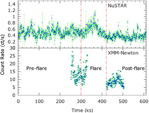
The X-ray light curves of NGC 4051 in 3–50 keV and 0.3–10 keV ranges, obtained from the 2018 November NuSTAR (upper panel) and XMM–Newton (bottom panel) observations, respectively, are shown for 500-s time bins. In the NuSTAR light curve, a flare of ∼120 ks duration with peak count rate reaching by a factor of ∼2.5 compared with the quiescent duration is detected. The red dotted lines divide the light curves (observations) into three time intervals representing pre-flare, flare, and post-flare segments.
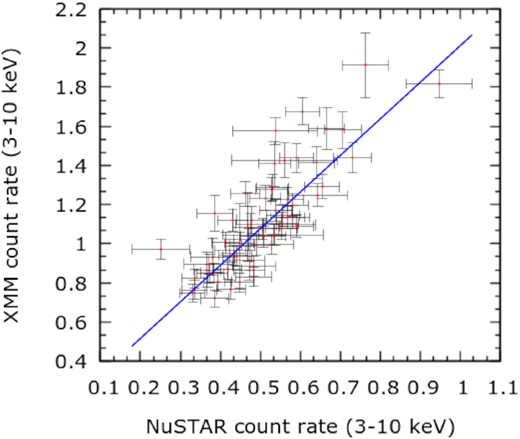
The count rates in the 3–10 keV range are shown for the overlapping pre-flare phase of the XMM–Newton and NuSTAR observations.
3 DATA ANALYSIS AND RESULTS
3.1 Timing analysis
3.1.1 Fractional variability
Firs, we attempted to investigate the timing variability of NGC 4051 using XMM–Newton and NuSTAR observations. To check the temporal variability, we calculated the fractional variability (Fvar: Nandra et al. 1997; Vaughan et al. 2003) in different energy bands using the equation
and the uncertainty in Fvar as
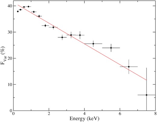
where |$\bar {x}$|, S, |$\overline{\sigma }_{\rm err}$|, and N are the mean, total variance, mean error, and number of data points, respectively. We generated the variability spectrum, i.e. Fvar as a function of energy (see Fig. 3), using background-subtracted EPIC-pn (Obs. ID 0830430201) light curves in increasing energy binning. Pearson’s correlation coefficient was calculated to be −0.95 with a null hypothesis probability of ∼10−9. The spectrum shows that the low-energy components, e.g. soft X-ray excess or/and ionized absorbers, are more variable than the high-energy ones.
The fractional variability spectrum is shown for the EPIC-pn data from the XMM–Newton observation (Obs. ID 083043201) of NGC 4051. The red line represents the linear fit to the observed data points.
To have an initial guess for the spectral variability during the observations, we plotted the variation of the hardness ratio (HR), i.e. the ratio between the hard X-ray and soft X-ray light curves, with respect to time. For the NuSTAR observations, we computed HR by taking the ratio between the light curves in the 10–50 keV and 3–10 keV energy ranges, whereas for the XMM–Newton observation we estimated HR by taking the ratio between the 2–10 keV and 0.3–2 keV light curves. From Fig. 4, we observed considerable spectral variability in soft X-rays. The spectrum became soft at the beginning of the flare. Having observed closely, we find the ‘softer when brighter’ trend, which is corroborated by the hardness–intensity diagram (HR versus total count rate) in Fig. 5. On the other hand, the variability seen in the NuSTAR spectrum is comparatively less. The NuSTARHR is more or less constant except for softening marginally during the flaring phase (see the upper panel of Fig. 4 and left panel of Fig. 5).
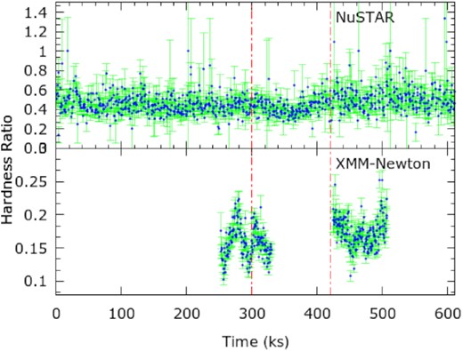
The hardness ratios are shown for NuSTAR (upper panel) and XMM–Newton (bottom panel) observations of NGC 4051. The hardness ratios are obtained by taking the ratio between the light curves in 10–50 keV and 3–10 keV bands (for NuSTAR) and 2–10 keV and 0.3–2 keV bands (for XMM–Newton).
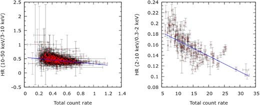
Hardness–intensity diagrams of NGC 4051 are shown using the NuSTAR (left panel) and XMM–Newton (right panel) observations. Corresponding correlation coefficients are −0.42 and −0.73, respectively.
3.1.2 Correlation
For correlation analysis in the X-ray band (3.0–50.0 keV), we divided the entire set of NuSTAR observations of NGC 4051 into pre-flare (MJD 58426.5–58430.0), flare (MJD 58430.0–58431.4), and post-flare (MJD 58431.4–58433.6) segments, which are marked with vertical lines in Fig. 1. For each segment, we segregated the X-ray light curve into soft X-ray (3.0–10.0 keV) and hard X-ray (10.0–50.0 keV) bands. Corresponding light curves with a time resolution of 50 s are shown in the top panels of Fig. 6. During the entire duration of the observations, the source count rate in the hard X-ray band was always less than that of the soft X-ray band. At the peak of the flaring event, the source count rate in both bands increased by a factor of 2–3 compared with the average count rate during the pre-and post-flare segments. We performed cross-correlation analysis using crosscor2 and the ζ-discrete cross-correlation function (ZDCF:3 Alexander 1997) for comparison of light curves in two different bands. For the error estimation, we considered 12 000 simulation points in the ZDCF code for the light curves. The soft- and hard-band light curves during the pre- and post-flare segments yielded an acceptable |$\rm \chi ^2_{red} \lt 1.5$| when fitted with a straight line. However, the data during the flare yielded poor statistics with high residuals when fitted with a linear function. We carried out delay estimation through the discrete correlation function using NuSTAR data during the three segments separately.
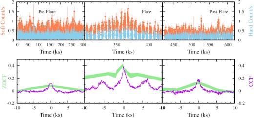
Top panel: light curves of NGC 4051 in the soft X-ray (3.0–10.0 keV: salmon) and hard X-ray (10.0–50.0 keV: light blue) bands obtained from NuSTAR observations are shown for pre-flare, flare, and post-flare segments. Bottom panel: discrete cross-correlations between the soft X-ray and hard X-ray light curves are plotted. A moderately strong correlation between these bands can be seen during the duration of the flare, which is absent in the pre-and post-flare segments. The cross-correlation functions (CCFs) are presented with a solid magenta line, whereas the green bands represent the ζ-discrete cross-correlations.
Discrete correlation function analysis, performed on the light curves from the three different segments, generated three different patterns as shown in the bottom panels of Fig. 6. In the pre- and post-flare phases, the soft and hard X-ray bands are found to be very poorly correlated. The values of the correlation function for pre-flare and post-flare segments were found to be <0.1 (left bottom panel of Fig. 6) and <0.2 (right bottom panel of Fig. 6), respectively, for a time delay range of −10 to +10 kiloseconds (ks). However, the flaring-event data showed a moderately strong correlation between the soft and hard bands in both algorithms. From the ZDCF, we found the peak of the correlation function at 0.0 ± 0.05 ks with a correlation coefficient of 0.48 ± 0.02, and for the CCF, calculated through crosscor, the peak appears at 0.0 ± 0.05 with a correlation coefficient of 0.4 (middle bottom panel of Fig. 6). Although, from the CCF analysis of post-flare segment data, a minor peak is observed near 0.0 ± 50 ks time delay, it is not prominent, as the peak value is 0.13 (bottom right panel of Fig. 6). Therefore, we are not considering this as a peak in the correlation function. We do not notice any significant peak in the ζ-discrete cross-correlation function in this post-flaring segment. From the correlation analysis, we conclude that the soft and hard X-ray light curves are moderately correlated only during the flare segment.
3.2 Spectral analysis
We used the xspec (v12.11.1) software package (Arnaud 1996) to analyse the spectral data and χ2 statistics to find the best-fitting models. Throughout spectral analysis, the uncertainties in various parameters are calculated using the error command in xspec at 90 per cent confidence level unless otherwise stated. As mentioned earlier, the data from the NuSTAR and XMM–Newton observations are divided into three segments: pre-flare, flare, and post-flare (see Fig. 1). We carried out the spectral analysis in the 0.3–50 keV energy range using simultaneous XMM–Newton and NuSTAR observations for all three segments.
The X-ray spectrum of an AGN is typically described by a power-law continuum, complex iron emission lines in the ∼6–7 keV range, reflection hump in the ∼20–40 keV range, and soft X-ray excess below 2 keV. We used various phenomenological as well as physical models and included all the features in our analysis. We used zpowlw,4borus (Baloković et al. 2018), and relxilllpion, a modified version of the relxill5 model (Dauser et al. 2016). For Galactic absorption and local ionized absorption, we used the phabs or tbabs (Wilms, Allen & McCray 2000) and zxipcf6 models, respectively.
We started our spectral analysis with NuSTAR observations in the 3–50 keV range to have an initial idea of spectral changes with flux variability. As mentioned earlier, we dissected the NuSTAR observations into three parts: pre-flare, flare, and post-flare segments. To investigate the spectral changes during the flare, we further divided the flare duration into two sub-segments, the rising and declining phases. Our basic model reads in xspec as
In the above expression, we used the cut-off power-law model to fit the primary continuum. In this model, ‘constant’ stands for the relative normalization of leaked or scattered unabsorbed intrinsic continuum. The zphabs × cabs component represents line-of-sight absorption, including Compton scattering losses out of the line of sight. Here, the additive borus model is used for reprocessed emission from cold and neutral gas. This model calculates the fluorescent line emission and reprocessed continuum self-consistently. We simultaneously fitted all four time-resolved spectra with the above model. While fitting, the inclination angle, covering factor (|$C_{\rm F, Tor}$|), and average column density (|$N_{\rm H,Tor}$|) of the obscuring materials are tied across the four segments. These parameters are unlikely to change during such a short observation span. The foreground Galactic absorption column density is fixed at NH, Gal = 1.2 × 1020cm−2 (HI4PI Collaboration et al. 2016) in the source direction and modelled with phabs. We obtained a good fit (χ2/dof = 1669/1603) with this model. All the fitted parameters are listed in Table 2. From this fitting, we found that the photon index (Γ) was relatively higher during the flare phase compared with the pre- and post-flare phases. We could not constrain the cut-off energy (Ecut) in all four phases. The inclination angle obtained from this fitting was found to be around 30 degrees, which is reasonable for type 1 Seyfert galaxies. The best fitted spectrum has been shown in Fig. 7.
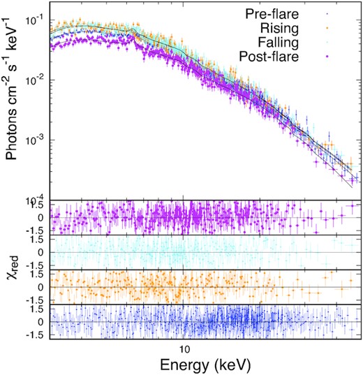
Top panel: The best-fitting model spectra (fitted simultaneously) for the pre-flare, rising, and falling parts of the flare, post-flare phases in the 3–50 keV energy range from NuSTAR observations. The bottom four panels show the corresponding residuals. The magenta, cyan, orange, and green points represent the data from the pre-flare, rising part of the flare, declining part of the flare, and post-flare phases, respectively.
The best-fitted parameters obtained by fitting the 3–50 keV NuSTAR time-resolved spectra of NGC 4051 with the borus model.
| Parameters | Pre-flare | Rising | Declining | Post-flare |
|---|---|---|---|---|
| segment | phase | phase | segment | |
| |$N_{\rm H, \rm Tor}$| (1022 cm−2) | |$24.50_{-0.06}^{+0.07}$| | |$\rm f$| | |$\rm f$| | |$\rm f$| |
| |$C_{\rm F, \rm Tor}$| | |$0.87_{-0.03}^{+0.07}$| | |$\rm f$| | |$\rm f$| | |$\rm f$| |
| Incl (deg.) | |$30_{-5}^{+5}$| | |$\rm f$| | |$\rm f$| | |$\rm f$| |
| AFe | |$1.10_{-0.14}^{+0.33}$| | |$0.97_{-0.23}^{+0.27}$| | |$1.01_{-0.28}^{+0.35}$| | |$0.82_{-0.17}^{+0.22}$| |
| Norm (10−3) | |$6.20_{-1.10}^{+1.10}$| | |$7.42_{-0.92}^{+0.32}$| | |$8.09_{-1.00}^{+0.66}$| | |$3.29_{-0.73}^{+1.30}$| |
| |$N_{\rm H, \rm ref}$| (1022 cm−2) | |$1.22_{-0.55}^{+0.50}$| | <0.62 | |$0.83_{-0.70}^{+0.59}$| | 1† |
| Γ | |$1.89_{-0.08}^{+0.06}$| | |$1.97_{-0.09}^{+0.05}$| | |$1.97_{-0.08}^{+0.03}$| | |$1.64_{-0.07}^{+0.09}$| |
Notes. |$\rm f$| represents a parameter fixed at the corresponding value at the pre-flare phase.
† pegged at this value.
It was found that the photon index remained unchanged during the rising and declining phases of the flare. Therefore, we clubbed these two time intervals together for further spectral analysis. Next, we fitted simultaneous XMM–Newton (0.3–10 keV range) and NuSTAR (3–50 keV range) spectra in the three segments (pre-flare, flare, and post-flare) together using different models. The advantage of fitting spectra of three intervals simultaneously is that it produces spectral variability in a more physical way.
Model 1: We built our baseline model with a power law with a high-energy cut-off as the source continuum. We used a redshifted blackbody component (zbbody) for the soft excess, a Gaussian line (zgaus) for the Fe Kα emission line, and the pexrav model for the reflection component above 10 keV (Magdziarz & Zdziarski 1995). We set the reflection fraction (Rrefl) as negative so that the pexrav component is considered as only the reflection spectrum. We fixed the inclination angle at 30 degrees as obtained from the previous model. The iron and heavy-element abundances were tied for three intervals. The photon index of the pexrav model was linked with that of the cut-off power-law model. Since the cut-off energy could not be constrained, we fixed it at 370 keV for low-Eddington Seyfert galaxies as suggested in the statistical study by Ricci et al. (2017). We needed two absorbers while fitting the spectra to obtain the best-fitting model. The final model in xspec reads
We applied a constant factor in the composite model to take into account the calibration uncertainties between different instruments. This model provided a good fit to the XMM–Newton and NuSTAR data, with χ2 = 5385 for 5104 degrees of freedom (dof). We required two ionized absorbers for the residuals below 2 keV. To take into account this absorption feature, we included two zxipcf models for partially covering and partially ionized absorbing material. The redshift (z ∼ −0.20) obtained for the first absorber was similar to that for ultrafast outflows (UFOs: Tombesi et al. 2013) during the three intervals. The second absorber showed a redshift comparable to that of warm absorbers (WAs: Blustin et al. 2005). The value of the blackbody temperature was found to be ∼100 eV, which was non-variable during the observation period. The spectrum became softer during the flare, with the best-fitting photon-index Γ = 2.10 ± 0.01. As we are considering only the reflection component of the pexrav model and using a separate continuum model, we could not constrain the value of the reflection scaling factor and fixed it at −1. All the best fitted parameters are listed in Table 3. We calculated the soft excess and power-law flux from the corresponding model components. The soft excess flux was found to be decreasing with time, while the power-law flux was highest during the flaring phase. The best fitted spectrum has been shown in Fig. 8 (a).
The best-fitting parameters obtained from fitting 0.3–50 keV time-resolved spectra simultaneously using XMM–Newton and NuSTAR observations with phenomenological model zcut-offpl.
| Parameters | Pre-flare | Flare | Post-flare |
|---|---|---|---|
| segment | segment | segment | |
| NH, 1 (1022 cm−2) | |$9.38_{-1.61}^{+1.22}$| | |$14.87_{-2.86}^{+2.47}$| | |$11.13_{-1.69}^{+1.65}$| |
| |$\log {\rm \xi _{\rm 1}}$| | |$1.08_{-0.95}^{+0.08}$| | |$1.09_{-0.56}^{+0.14}$| | |$1.31_{-0.09}^{+0.06}$| |
| Cov Frac1 | |$0.24_{-0.01}^{+0.02}$| | |$0.20_{-0.01}^{+0.02}$| | |$0.23_{-0.03}^{+0.01}$| |
| z1 | |$-0.20_{-0.06}^{+0.04}$| | |$-0.21_{-0.07}^{+0.04}$| | |$-0.22_{-0.05}^{+0.02}$| |
| ν/c | −0.20 | −0.21 | −0.22 |
| rmax (pc) | 0.17 | 0.11 | 0.06 |
| rmin (10−4 pc) | 0.04 | 0.04 | 0.03 |
| rmin (Rs) | 25 | 23 | 21 |
| NH, 2 (1022 cm−2) | |$0.62_{-0.51}^{+0.52}$| | |$2.28_{-0.89}^{+0.79}$| | |$2.99_{-0.55}^{+0.52}$| |
| |$\log {\rm \xi _{\rm 2}}$| | |$2.07_{-0.45}^{+0.15}$| | |$2.08_{-0.14}^{+0.14}$| | |$2.01_{-0.03}^{+0.07}$| |
| Cov Frac1 | |$0.39_{-0.09}^{+0.58}$| | |$0.30_{-0.05}^{+0.07}$| | |$0.40_{-0.02}^{+0.03}$| |
| z2 | |$0.04_{-0.02}^{+0.02}$| | |$0.02_{-0.02}^{+0.02}$| | |$0.03_{-0.01}^{+0.01}$| |
| ν/c | 0.04 | 0.02 | 0.03 |
| rmax (pc) | 0.26 | 0.07 | 0.04 |
| rmin (10−4 pc) | 1.20 | 0.40 | 1.08 |
| min (Rs) | 730 | 3460 | 1372 |
| kTBB (eV) | |$100_{-1}^{+1}$| | |$100_{-2}^{+2}$| | |$100_{-1}^{+1}$| |
| NormBB (10−04) | |$1.50_{-0.02}^{+0.02}$| | |$1.11_{-0.22}^{+0.25}$| | |$0.85_{-0.01}^{+0.01}$| |
| Fe Kα LE (keV) | |$6.40_{-0.03}^{+0.02}$| | |$6.36_{-0.05}^{+0.04}$| | |$6.35_{-0.02}^{+0.02}$| |
| EW (eV) | |$101_{-15}^{+16}$| | |$82_{-20}^{+22}$| | |$95_{-32}^{+29}$| |
| Norm (10−5) | |$1.97_{-0.29}^{+0.32}$| | |$1.58_{-0.38}^{+0.42}$| | |$1.35_{-0.23}^{+0.23}$| |
| Abund | |$1.87_{-0.16}^{+0.18}$| | |$\rm f$| | |$\rm f$| |
| AbundFe | |$2.39_{-0.21}^{+0.22}$| | |$\rm f$| | |$\rm f$| |
| Γ | |$2.05_{-0.01}^{+0.01}$| | |$2.10_{-0.01}^{+0.01}$| | |$2.05_{-0.01}^{+0.01}$| |
| NormPL (10−03) | |$7.82_{-0.02}^{+0.02}$| | |$8.34_{-0.03}^{+0.03}$| | |$5.43_{-0.01}^{+0.01}$| |
Note. |$\rm f$| represents a parameter fixed at the corresponding value at the pre-flare phase.
Model 2: Time-resolved spectral fitting of NuSTAR and XMM–Newton data with Model 1 provided information on the spectral changes, presence of warm absorbers, and UFO in the three time intervals. However, it did not provide any physical properties of the Comptonizing plasma, i.e. the corona. To get information on the change in coronal properties, we replaced zcut-offpl with the Comptonization model compPS (Poutanen & Svensson 1996). This model produces an X-ray continuum for different geometries using the exact numerical solution of the radiative transfer equation, which depends on the geometry, optical depth of the hot electron plasma, spectral distribution of the seed photons, inclination angle, and the way seed soft photons are injected into the hot plasma. This model also takes into account the reflection spectra from the cold medium as well as the blurred reflection smeared out by the rotation of the disc and relativistic effects. In the fitting process, we fixed certain parameters based on a prior guess of the system so that fitting could converge. The composite model in xspec reads
We considered a spherical geometry of the plasma in this model. The inclination was fixed at 30 degrees. The values of |$\rm R_{in}$| and |$\rm R_{out}$| were fixed at 6 and 2000|$R_\mathrm{ s}$|, respectively. The best fitted spectrum has been shown in Fig. 8 (b). The parameters obtained from fitting the data from three segments are tabulated in Table 4. Instead of the optical depth, this model incorporates the Compton y-parameter (τy) as one input, which relates to the optical depth as τ = τy/(4kTe/mec2), where kTe is the hot electron temperature in keV. Iron and heavy-element abundances were tied for the time intervals. The absolute value of Fe Kα line energy varies marginally during the three phases, while the equivalent width (EW) is lowest in the flare phase. The inner disc temperature is found to be invariable (within error) with an average temperature of ∼18 eV. From this model, interestingly, we found that the coronal temperature increased to ∼228 keV post-flare, while it was similar before and during the flare with a value of around ∼182 keV. Moreover, the reflection fraction was found to be decreasing during the flare, while it increased substantially after the flare.
The best-fitting parameters obtained after fitting 0.3–50 keV time-resolved spectra simultaneously using XMM–Newton and NuSTAR observations with phenomenological model compPS.
| Parameters | Pre-flare | Flare | Post-flare |
|---|---|---|---|
| segment | segment | segment | |
| NH, 1 (1022 cm−2) | |$8.22_{-0.87}^{+0.25}$| | |$7.55_{-1.47}^{+1.17}$| | |$5.64_{-0.26}^{+0.36}$| |
| |$\log {\rm \xi _{\rm 1}}$| | |$1.93_{-0.02}^{+0.09}$| | |$1.89_{-0.04}^{+0.07}$| | |$1.80_{-0.06}^{+0.02}$| |
| Cov Frac1 | |$0.35_{-0.02}^{+0.01}$| | |$0.28_{-0.05}^{+0.07}$| | |$0.45_{-0.02}^{+0.03}$| |
| z2 | |$-0.26_{-0.01}^{+0.01}$| | |$-0.26_{-0.02}^{+0.02}$| | |$-0.21_{-0.01}^{+0.01}$| |
| NH, 2 (1022 cm−2) | |$0.47_{-0.08}^{+0.43}$| | |$1.37_{-0.76}^{+2.02}$| | |$1.24_{-0.54}^{+0.32}$| |
| |$\log {\rm \xi _{\rm 2}}$| | |$2.15_{-0.06}^{+0.08}$| | |$2.14_{-0.09}^{+0.13}$| | |$2.04_{-0.05}^{+0.08}$| |
| Cov Frac2 | >0.63 | >0.47 | |$0.71_{-0.06}^{+0.16}$| |
| z1 | |$0.001_{-0.01}^{+0.01}$| | |$0.01_{-0.01}^{+0.02}$| | |$0.04_{-0.01}^{+0.01}$| |
| Fe Kα LE (keV) | |$6.40_{-0.03}^{+0.02}$| | |$6.37_{-0.05}^{+0.04}$| | |$6.35_{-0.02}^{+0.02}$| |
| σ (eV) | |$97_{-49}^{+55}$| | |$115_{-58}^{+88}$| | |$70_{-41}^{+38}$| |
| EW (eV) | |$125_{-17}^{+18}$| | |$101_{-22}^{+25}$| | |$118_{-18}^{+19}$| |
| Norm (10−05) | |$2.38_{-0.33}^{+0.35}$| | |$1.82_{-0.39}^{+0.44}$| | |$1.56_{-0.23}^{+0.24}$| |
| kTe (keV) | |$182_{-23}^{+24}$| | |$184_{-26}^{+28}$| | |$228_{-15}^{+52}$| |
| kTbb (eV) | |$19_{-3}^{+3}$| | |$19_{-4}^{+5}$| | |$16_{-3}^{+4}$| |
| τy | |$0.37_{-0.02}^{+0.02}$| | |$0.36_{-0.03}^{+0.03}$| | |$0.31_{-0.01}^{+0.02}$| |
| relrefl | |$2.19_{-0.16}^{+0.16}$| | |$2.10_{-0.23}^{+0.21}$| | |$2.58_{-0.46}^{+0.29}$| |
| Abund | |$4.68_{-0.41}^{+0.47}$| | |$\rm f$| | |$\rm f$| |
| AbundFe | |$2.25_{-0.30}^{+0.29}$| | |$\rm f$| | |$\rm f$| |
Note. |$\rm f$| represents a parameter fixed at the corresponding value at the pre-flare phase.
We also tried the bmc model (Titarchuk, Mastichiadis & Kylafis 1997; Titarchuk & Zannias 1998; Laurent & Titarchuk 1999) for fitting the data. This model describes the spectrum generated not only by thermal Comptonization but also by the Comptonization of soft photons due to matter going through relativistic bulk motion. This is the self-consistent convolution model of power-law and seed blackbody soft photons. The resultant spectrum is characterized by the spectral index, α (= Γ − 1), seed photon temperature (kT), and an illumination parameter (A), which is the fractional illumination of bulk-motion flow by thermal photons. The composite model in xspec reads
Here, we used zbbody to fit the high-energy hump above 10 keV. The fitted model parameters are listed in Table 5.
The best-fitting parameters obtained after fitting 0.3–50 keV time-resolved spectra simultaneously using XMM–Newton and NuSTAR observations with the bmc model.
| Parameters | Pre-flare | Flare | Post-flare |
|---|---|---|---|
| segment | segment | segment | |
| kT (eV) | |$9.44_{-0.10}^{+0.10}$| | |$9.30_{-0.15}^{+0.15}$| | |$9.28_{-0.12}^{+0.11}$| |
| alpha | |$1.10_{-0.01}^{+0.01}$| | |$1.15_{-0.01}^{+0.01}$| | |$1.10_{-0.01}^{+0.01}$| |
| log A | |$0.05_{-0.01}^{+0.01}$| | |$0.20_{-0.02}^{+0.02}$| | |$0.13_{-0.01}^{+0.01}$| |
| Normbmc (10−04) | |$4.30_{-0.02}^{+0.02}$| | |$4.12_{-0.02}^{+0.02}$| | |$2.61_{-0.01}^{+0.01}$| |
| kThump (keV) | |$9.12_{-0.47}^{+0.53}$| | |$9.68_{-0.81}^{+0.97}$| | |$7.69_{-0.46}^{+0.51}$| |
| Normhump (10−04) | |$1.97_{-0.14}^{+0.16}$| | |$1.77_{-0.21}^{+0.25}$| | |$1.46_{-0.12}^{+0.13}$| |
Note. kThump is the temperature of the blackbody component used for the hump above 10 keV.
Using the correlation of the photon index and bmc normalization, the mass of the black hole can be estimated. This concept has been discussed in detail and implemented for NGC 4051 in Seifina et al. (2018). The expression used by Seifina et al. (2018) to calculate the mass of the black hole is given by
where M, N, and d are the black hole mass, normalization, and distance of the source, respectively. In this equation, the subscript t represents the target source, whereas r represents the reference source. Here, fG = cos(θr)/cos(θt) is a geometrical factor that takes into consideration the difference in viewing angles of the inner disc from which the seed photons are being emitted for both target and reference sources. θ is the inclination angle of the inner disc, which has been taken equal to the inclination angle of the source. Here, we consider NGC 4051 as the target source and GRO J1655–40 as the reference source. Referring to the Seifina et al. (2018) estimations of GRO J1655–40, Nr = 7 × 10⁻², θr = 70 degrees, and dr = 3.2 kpc and, using our estimate of normalization for NGC 4051 as Nt ≈ 4 × 10⁻⁴ and θt = 30 degrees, we calculate the black hole mass in NGC 4051 as ≥1.32 × 10⁵ M⊙ for a source distance of dt = 9800 kpc (Seifina et al. 2018). Our estimated value of the black hole mass in NGC 4051 is lower than that estimated by Seifina et al. (2018) (6.1 × 10⁵ M⊙). The discrepancy in estimated values of the black hole mass in NGC 4051 is due to the difference in the values of fG and Nt. Seifina et al. (2018) used fG and Nt values of 1 and ≈8.1 × 10⁻³, whereas from our analysis the value of fG is estimated to be 0.39.
Model 3: Reflection from the photoionized accretion disc is considered to be one of the explanations for the origin of the soft X-ray excess in AGNs. Emission from a compact, hot, and relativistic plasma irradiates the accretion disc. The X-ray illumination is stronger in the inner regions of the accretion disc, due to the strong gravity of the central black hole. We used the relxilllpion variant of the relxill model to describe the soft X-ray excess. The relxill model computes the continuum emission and its reflection from the accretion disc, which includes the reprocessing of continuum photons in the disc. The blurring of soft X-ray emission lines due to relativistic motion of the inner disc gives a smooth curvature, which appears as a soft X-ray excess. This model is parameterized by the inclination angle, inner radius, reflection fraction, and ionization parameter (|$\rm log\xi$|), with constant ionization throughout the disc. The relxilllpion model allows the ionization of the disc to vary with radius, and this variation is approximated by a power law. The composite model in xspec reads
While fitting the data with this model, we tied the iron abundance across the three intervals. The Eddington ratio for this source is calculated to be ∼0.01 for a black hole mass of 1.73 × 10⁶ M⊙ and bolometric luminosity ∼2.3 × 1042 erg s−1. The cut-off energy is kept fixed at 370 keV as earlier. We required two absorbers to fit the residuals in the soft X-ray range (<2 keV) of the spectra. Initially, we varied the values of inner disc radius (|$R_{\rm in}$|) and ionization parameter (|$\rm log\xi$|) and found fairly unchanged parameter values. Therefore, we tied these parameters for all three segments. The height of the corona from the disc increased to |$12.18_{-0.92}^{+0.98}$|Rg, accompanied by a reduction in the reflection fraction during the flare. After the flare, the coronal height decreased, with the highest reflection fraction among the three phases. The best fitted spectrum has been shown in Fig. 8 (c).
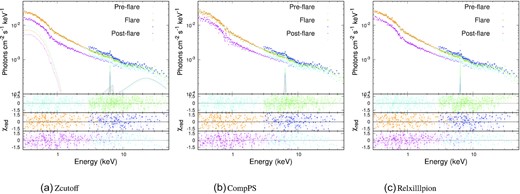
Top panel: 0.3–50 keV XMM–Newton + NuSTAR spectra fitted with Model 1 (left panel), Model 2 (middle panel), and Model 3 (right panel) for the pre-flare, flare, and post-flare phases. Bottom three panels: corresponding residuals for the pre-flare, flare, and post-flare phases, respectively. The cyan, orange, and magenta points represent the XMM–Newton data for the pre-flare, flare, and post-flare phases, respectively. The green, blue and turquoise points represent the NuSTAR data for the pre-flare, flare, and post-flare phases, respectively.
4 DISCUSSION
In this work, we explored the changes in the spectral and timing properties of NGC 4051 during the pre-flare, flare, and post-flare phases using data obtained from XMM–Newton and NuSTAR observations in 2018 November. We explored the accretion properties, accretion mechanism, and corona structural changes of the source in detail using various phenomenological and physical models. The results obtained from our work are described here.
4.1 Black hole spin
The spin of the black hole is estimated self-consistently from the X-ray reflection models. In the present work, the spin parameter was linked while fitting the spectra of three segments simultaneously. From the relativistic reflection model relxilllpion, we found that the black hole is spinning rapidly with spin parameter a > 0.85, while keeping the values of the inner radius and spin parameter tied for all three time intervals.
4.2 Location of the absorbers
While fitting the spectra from simultaneous observations of NGC 4051 with XMM–Newton and NuSTAR, we required two absorbers to get rid of the residuals below 2 keV in all the spectral models used in this work. We took into account absorption with partially ionized and partially covered absorber model zxipcf. The properties of these absorbers are listed in Tables 3, 4, and 6. The ionization parameter of an absorber is defined as ξ = Lion/nr2 (Tarter, Tucker & Salpeter 1969), where Lion, n, and r are the unabsorbed ionizing luminosity of the emitting source, number density, and radial location of the absorber from the central source, respectively. The absorption from the excited states or absorption variability can be used to determine the limits of r using the definition of ξ. It is possible to estimate the upper limit of the radial distance based on the assumption that the thickness of the absorber cannot exceed its location from the SMBH (Blustin et al. 2005; Crenshaw & Kraemer 2012):
where NH is the column density of the absorber.
The best-fitting parameters obtained after fitting 0.3–50 keV time-resolved spectra simultaneously using XMM–Newton and NuSTAR observations with physical model relxilllpion.
| Parameters | Pre-flare | Flare | Post-flare |
|---|---|---|---|
| segment | segment | segment | |
| NH, 1 (1022 cm−2) | |$21.04_{-2.39}^{+4.79}$| | |$46.46_{-4.09}^{+4.89}$| | |$47.59_{-9.00}^{+6.93}$| |
| |$\log {\rm \xi _{\rm 1}}$| | |$1.92_{-0.07}^{+0.08}$| | |$2.00_{-0.03}^{+0.03}$| | |$1.77_{-0.30}^{+0.23}$| |
| Cov Frac1 | |$0.27_{-0.02}^{+0.02}$| | |$0.30_{-0.01}^{+0.01}$| | |$0.30_{-0.01}^{+0.01}$| |
| z1 | |$-0.33_{-0.02}^{+0.01}$| | |$-0.31_{-0.02}^{+0.03}$| | |$-0.36_{-0.03}^{+0.02}$| |
| NH, 2 (1022 cm−2) | |$3.98_{-0.59}^{+0.59}$| | |$5.44_{-0.47}^{+0.39}$| | |$1.07_{-0.30}^{+0.11}$| |
| |$\log {\rm \xi _{\rm 2}}$| | |$1.91_{-0.06}^{+0.09}$| | |$1.98_{-0.11}^{+0.08}$| | |$1.90_{-0.07}^{+0.04}$| |
| Cov Frac1 | |$0.28_{-0.02}^{+0.03}$| | |$0.35_{-0.03}^{+0.02}$| | |$0.45_{-0.01}^{+0.01}$| |
| z2 | |$-0.01_{-0.01}^{+0.02}$| | |$-0.01_{-0.02}^{+0.01}$| | |$0.001_{-0.008}^{+0.007}$| |
| h | |$9.61_{-1.68}^{+1.38}$| | |$12.18_{-0.92}^{+0.98}$| | |$7.36_{-0.98}^{+1.51}$| |
| a | >0.85 | |$\rm f$| | |$\rm f$| |
| Rin | <2.52 | |$\rm f$| | |$\rm f$| |
| |$\log {\rm \xi _{\rm 1}}$| | |$3.10_{-0.06}^{+0.05}$| | |$\rm f$| | |$\rm f$| |
| Γ | |$2.16_{-0.01}^{+0.01}$| | |$2.18_{-0.01}^{+0.01}$| | |$2.15_{-0.01}^{+0.01}$| |
| AbundFe | |$1.02_{-0.04}^{+0.16}$| | |$\rm f$| | |$\rm f$| |
| Refl. frac | |$2.00_{-0.06}^{+0.06}$| | |$1.42_{-0.05}^{+0.05}$| | |$2.12_{-0.06}^{+0.07}$| |
| Ionization index | |$1.07_{-0.05}^{+0.08}$| | |$1.15_{-0.09}^{+0.09}$| | |$1.03_{-0.05}^{+0.05}$| |
| NormPL (10−4) | |$1.79_{-0.72}^{+0.71}$| | |$1.91_{-0.05}^{+0.06}$| | |$1.73_{-0.18}^{+0.19}$| |
Note. |$\rm f$| represents a parameter fixed at the corresponding value at the pre-flare phase.
A lower limit on the location of the outflow can be calculated as
where G, MBH, and ν are the gravitational constant, black hole mass, and outflow velocity, respectively.
Another way of calculating the lower limit is by considering the light travel time D = Δt × c during the observation if the absorber does not seem to be variable. We used the values from the zcut-offpl model to estimate the radial location of both absorbers. The ionizing luminosity of this source has been calculated for three intervals by considering the power-law component in the 0.3–50 keV range (see Table 7). The locations of absorber 1 and absorber 2 are estimated and listed in Table 3 separately for three time intervals. These values of locations and redshifts are consistent with the WAs and UFOs found in studies of type 1 Seyfert galaxies (Tombesi et al. 2012, 2013).
Fluxes and luminosities.
| Parameters | Pre-flare | Flare | Post-flare |
|---|---|---|---|
| segment | segment | segment | |
| |$F_{\rm 0.3-2~keV}^{\rm BB} (10^{-12})\star$| | 7.65 ± 0.08 | 5.88 ± 0.09 | 4.54 ± 0.05 |
| |$F_{\rm 2-10~keV}^{\rm PL} (10^{-11})\star$| | 1.77 ± 0.01 | 1.82 ± 0.01 | 1.26 ± 0.06 |
| L0.1-200 (1041)• | 8.55 ± 0.03 | 9.20 ± 0.03 | 6.04 ± 0.02 |
| Lion (1041)• | 5.85 ± 0.02 | 6.18 ± 0.02 | 4.04 ± 0.01 |
| L2-10 keV (1041)• | 2.06 ± 0.01 | 2.39 ± 0.01 | 1.5 ± 0.01 |
| λEdd | 0.014 ± 0.001 | 0.016 ± 0.001 | 0.011 ± 0.001 |
| l | |$9.12_{-0.03}^{+0.02}$| | |$9.82_{-0.05}^{+0.02}$| | |$6.44_{-0.02}^{+0.03}$| |
| θ | |$0.36_{-0.04}^{+0.05}$| | |$0.36_{-0.06}^{+0.06}$| | |$0.45_{-0.03}^{+0.10}$| |
Note. ⋆ in units of erg s−1 cm−2, • in units of erg s−1.
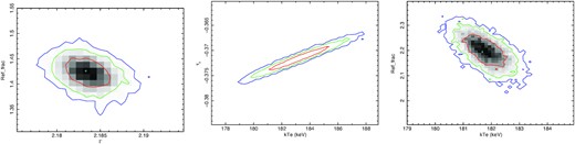
We have also calculated the marginal posterior distributions for the absorber parameters to check the spectral fitting degeneracy between them. To search through parameter space, we used the Markov Chain Monte Carlo (MCMC) sampling procedure. We used the Goodman & Weare (2010) algorithm implemented in xspec to determine the chain. We considered 20 walkers with a total chain length of 200 000 and burnt the initial 20 000 steps. The one-dimensional (1D) and two-dimensional (2D) distributions are shown in Fig. 9.

The 1D and 2D posterior distribution curves resulting from the MCMC analysis of the ionization paramter (log ξ), covering factor, and redshift (z) of the two absorbers. The vertical lines in the 1D distribution show 16, 50, and 90 per cent quantiles. CORNER.PY (Foreman-Mackey 2016) was used to plot the distributions.
4.3 Properties of the corona
The X-ray-emitting corona is characterized by the optical depth (τ), hot electron plasma temperature (|$kT_\mathrm{ e}$|), and X-ray continuum photon index (Γ). As the power-law with high-energy cut-off continuum model gives information only on the photon index, we utilized the compPS model, which considers |$kT_\mathrm{ e}$|, the Compton y-parameter, and the inner disc temperature (kTbb) as free parameters. We find that the temperature of the corona increased after the flare subsided and the source went into the low flux state. During the flare, when flux was high, the slope of the spectrum became steep. This softening of the X-ray continuum with high flux is consistent with the ‘softer when brighter’ nature observed in many AGNs (Connolly et al. 2016). The less energetic seed photons from the accretion disc get Comptonized in the corona, producing X-ray emission. In the present work, it is found that the coronal temperature increases after the flare. An increase in the temperature of the corona after the flare can be interpreted as due to the injection of fewer seed photons into the corona, resulting in the reduction of the Compton cooling rate. Considering the magnitude of the observed flare and the duration of the observation, it is highly unlikely that there could be any significant variation in the accretion rate (see |$\rm \lambda _{Edd}$| values from Table 7). Moreover, the flux of the soft X-ray excess (0.3–2 keV range) does not show any clear correlation with the photon index (see Table 7). This indicates that the change in spectral state during the flaring phase is inherent to the corona instead of due to variations in the seed photons. In an AGN, the corona is likely to be powered by the small-scale magnetic flux tubes associated with the orbiting plasma in the accretion disc (Yuan et al. 2019). Any change in the magnetic field can cause a change in the location and geometry of the corona, which in turn can result in coronal temperature variation. Recently, Wilkins et al. (2022) studied a similar kind of X-ray flaring event in NLS1 galaxy I Zw 1. They found that the temperature was higher in the pre-flare phase and decreased during the flare, probably due to the expansion of the corona accompanied by softening of the spectrum. After the flare, the temperature again started to increase with the hardening of the continuum spectrum. In NGC 4051, we found that the coronal temperature increased after the flare and the spectrum became harder. In this case, the corona perhaps started inflating in the pre-flare phase and reached a maximum during the flare. After the flare, it again contracted, followed by an increase in temperature.
In the present work, the coronal temperature was found to be high (average value of ∼198 keV). This is likely the reason we could not constrain the cut-off energy for this source. From the best-fitting values of the coronal temperature (kTe) and Compton y-parameter (y) (although these two parameters are degenerate, as shown in the middle contour plot of Fig. 10), the value of optical depth (|$\tau ={\tau _y}/({4T_\mathrm{ e}/m_\mathrm{ e} c^2})$|) is calculated as 0.26 ± 0.04, 0.25 ± 0.04, and 0.17 ± 0.03 in the pre-flare, flare, and post-flare phases, respectively. These values of τ are consistent with the mean value obtained for a sample of 838 Swift/Burst Alert Telescope (BAT) AGNs (Ricci et al. 2018). The coronal temperature carries important information on the state of the X-ray-emitting plasma. The position of the AGN in the compactness–temperature (θ–l plane) space provides an insight into the dominant process in the corona (Fabian et al. 2015). In the corona of an AGN, the most significant processes are inverse Compton scattering, bremsstrahlung, and pair production. Among these, the dominant process is the one for which the cooling time is the shortest. The Comptonization process dominates when l > 3αfθ−1/2, where αf and θ are the fine-structure constant and coronal temperature normalized to the electron rest energy, respectively. Electron–proton coupling dominates when 3αfθ < l < 0.04θ−3/2, while for 0.04θ−3/2 < l < 80θ−3/2 electron–electron coupling becomes prominent. There is a regime in the θ–l plane where the pair-production process becomes a runaway process, depending on the corona shape and radiation mechanism. Stern et al. (1995) computed the position of these pair runaway lines for a slab corona. Svensson (1984) calculated this regime for isolated clouds and gave the condition for its occurrence when l ∼ 10θ5/2e1/θ. The compactness parameter is defined as
where L, R, σT, me, and c are the luminosity, radius of the corona, Thomson cross-section, mass of the electron, and speed of light, respectively. We estimated this parameter for NGC 4051, considering a power-law continuum luminosity extrapolated to the 0.1–200 keV band in three intervals and a radius of 10Rg (for standard sources: Fabian et al. 2015). The l and θ values are given in Table 7 and plotted in Fig. 11. NGC 4051 is found to be located at the edge of the pair runaway region corresponding to the slab corona. This suggests that the process is mostly dominated by pair production and annihilation. In a compact corona (l > 1), when the photons are highly energetic, a photon–photon collision generates an electron–positron pair. If the temperature reaches ∼1 MeV, the pair-production process becomes significant, thereby soaking up energy and limiting the further rise in temperature.
Contour plots resulting from the MCMC analysis of the relxilllpion, compPS models for the reflection fraction versus Γ (left panel) , Compton y-parameter ( τy) versus kT e (middle panel), and reflection fraction versus kT e (right panel).
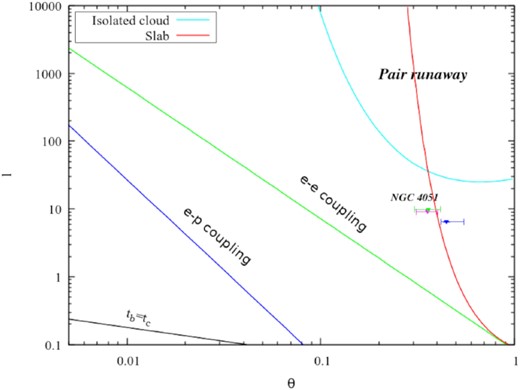
Theoretical compactness–temperature diagram is shown. The green line represents the region below which the electron–electron coupling time-scale is shorter than the Compton cooling time, while in the region below the blue line the electron–proton coupling time is shorter. Bremsstrahlung is dominant in the region below the black line. The region beyond the cyan and red curves represents where pair runaway processes occur for isolated cloud (Svensson 1984) and slab geometry (Stern et al. 1995). The green, magenta, and blue points are drawn for pre-flare, flare, and post-flare phase positions of NGC 4051, respectively.
4.4 Soft X-ray excess and reflection
A soft X-ray excess above the continuum is the most common feature seen in AGNs. This component is prominent in NLS1s. However, the origin of the soft X-ray excess is still under discussion. There are various models in the literature that take account of the origin of this component. Comptonization of photons in an optically thick and warm corona in the inner part of the disc is one explanation (Done et al. 2012) for the origin of the soft excess. Another scenario is one in which the photons from the hot corona (∼100 keV) are reflected from the relativistically moving inner accretion disc and give rise to a soft excess (Fabian et al. 2002; Ross & Fabian 2005; Pal et al. 2016). In the ionized absorption model, the photons are absorbed by high-velocity winds originating from the accretion disc and re-emitted (Gierliński & Done 2004).
In our analysis, we initially used the zbbody model to fit the soft X-ray excess. We found the blackbody temperature (|$kT_{\rm BB}$|) to be ∼ 100 eV, which was almost constant throughout the observation. This non-variation or minimal variation of the soft excess temperature is expected, as suggested by earlier studies (Gierliński & Done 2004; Ricci et al. 2017). We calculated the unabsorbed flux of the blackbody component for the soft excess and found it to be unaffected during the flare and decreasing with time (see Table 7).
From the relxilllpion model, we found that, during the flare, the reflection fraction decreased to 1.42 from 2.00 in the pre-flare phase and again increased to 2.09 in the post-flare phase. A similar trend was also observed from the compPS model. The change in the reflection component can be seen in Fig. 12, where the ratio between the 3–50 keV spectrum from the NuSTAR observations and the best-fitting power law is plotted. The reflection fraction is the ratio of reflected emission from the disc and continuum emission from the corona observed directly. From our analysis, we found this factor to be greater than unity, which means the source is reflection-dominated. Gravitational bending causes the X-rays to be concentrated towards the accretion disc, resulting in a high reflection fraction (Miniutti & Fabian 2004). As we mentioned above, NGC 4051 hosts a highly spinning black hole. Therefore, the effect of light bending causing a high reflection fraction is expected. In the simple lamppost geometry scenario, the compact corona is located above the central black hole. The drop in reflection fraction during the flare can be explained in terms of the coronal height from the accretion disc. We found that the coronal height increased, i.e. the corona moved away from the accretion disc, during the flare when the reflection fraction was lowest (second from top and bottom panels of Fig. 13). After the flare, the coronal height decreased and the reflection fraction increased again. Another possibility explaining the drop in reflection during the flare and enhancement after the flare could be a change in the inner accretion disc radius (De Marco et al. 2021). As mentioned before, we did not find any significant change in the inner radius during the three phases. Overionization could be another reason for the drop in reflection during the flare. However, the ionization parameter was invariant during the observation and was fixed for the final fitting. Therefore, motion of the corona away from the accretion disc seems to be the most plausible explanation for the variable reflection fraction.
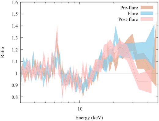
The ratio of the 3–50 keV spectrum from NuSTAR observations and best-fitting power-law model is shown. The varying strength of the reflection component above 10 keV is evident for all three phases of the observation.
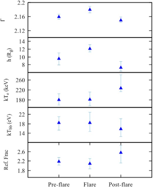
Variation of the best-fitting parameters is shown for three phases. The photon index (Γ), coronal height (h), and reflection fraction (R) are obtained from the relxilllpion model, while the coronal temperature (kTe) and inner disc temperature (kTbb) have been taken from the compPS model.
Reflection is one explanation for the observed hump in the spectrum above 10 keV. There is another interpretation of the hump put forth by Titarchuk & Seifina (2021). Laurent & Titarchuk (2007) studied the effect of Compton downscattering of continuum photons in the disc and concluded that the hump-like structure is only formed when the photon index Γ of the incident spectrum is less than 2. Laurent & Titarchuk (2018) claimed that when the photons gain energy up to 511 keV in the vicinity of the black hole, photon–photon interaction leads to pair production. The positrons that originate then interact with the electrons in a very narrow shell and emit annihilation-line photons. To an observer, due to high gravitational redshift (z ∼ 20), these line photons appear as a broad feature in the spectrum. The argument given in favour of this explanation is a shorter time-scale for hump emission compared with the iron emission line, as these two spectral features originate in geometrically different regions of the source. Hump emission comes from the region closer to the black hole, while the iron line is emitted from the region further away. We estimated the correlation functions between the 3–6, 6–7, and 10–50 keV energy bands, which are dominated by the power-law continuum, iron line, and hump or so-called reflection component in pre-flare, flare, and post-flare phases, respectively (Fig. 14). We found no correlation between the 6–7 and 10–50 keV energy bands in any of the phases, while a moderate correlation was found between the 3–6 and 6–7 keV energy bands and 3–6 and 10–50 keV energy bands in the pre- and post-flaring phases. This indicates that the hump and iron line could be of origins different from simple reprocessing of the continuum. Therefore, the annihilation-line photon scenario could be one possible origin of the hump-like spectral feature above 10 keV, often seen in Seyfert galaxies.
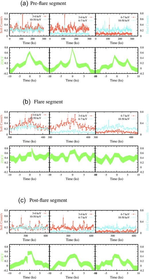
Light curves in the 3–6, 6–7, and 10–50 keV energy ranges and the correlation function between the light curves in two energy ranges are shown for (a) pre-flare, (b) flare, and (c) post-flare segments. For each segment, the light curves are shown in the upper panel, whereas the corresponding correlation function between the light curves is shown in the bottom panel.
5 SUMMARY AND CONCLUSIONS
A detailed broad-band X-ray spectral and timing analysis of a minor flaring event in NLS1 galaxy NGC 4051 during 2018 November 4–11 has been performed using simultaneous observations with the NuSTAR and XMM–Newton observatories. While analysing the data, we divided the total exposure into three phases: pre-flare, flare, and post-flare, and carried out timing and spectral studies during three segments. The main results and conclusions of our analysis are as follows.
NGC 4051 showed rapid variability in the 3–50 keV energy band of NuSTAR, where the count rate increased by a factor of ∼2.5, followed by a decrease to the pre-flare level within a day. The X-ray variability spectrum of the source showed a trend where variability is higher in soft bands, i.e. soft excess or ionized absorbers.
From spectral analysis in the 3–50 keV range, we found that the spectral slope changes during the observation period. During the flare, the 0.3–50 keV spectrum was softest.
During the X-ray flare, the reflection fraction is lowest, which is consistent with the increase in coronal height. After the flare, the coronal height reaches its lowest value during the observation with the increase in reflection fraction.
We find that the temperature of the corona increased significantly after the flare (see Fig. 13) from |$184_{-28}^{+26}$| to |$228_{-52}^{+15}$| keV. This reheating of the corona is consistent with the hardening of the spectra after the flare subsides.
In this source, we found signatures of warm absorbers and ultrafast outflows.
NGC 4051 hosts a rapidly spinning black hole with spin parameter a > 0.85 and black hole of mass ≥1.32 × 10⁵ M⊙.
NGC 4051 is positioned in the compactness–temperature plane at a region between electron–electron coupling and the pair runaway line for a slab corona. This implies that the dominant process in the corona is pair production.
Rapid spectral variabilities in NGC 4051 or similar types of NLS1 could be due to a change in the coronal geometry and/or location, which in turn produces small-scale flares. Due to the short time-scale of these flares, their origin in the corona is likely to be associated with the ejection of the magnetic field.
ACKNOWLEDGEMENTS
We thank the anonymous reviewer for suggestions that helped us to improve the manuscript. This research work at PRL is funded by the Department of Space, Government of India. AJ acknowledges the support of a grant from the Ministry of Science and Technology of Taiwan with grant numbers MOST 110-2811-M-007-500 and MOST 111-2811-M-007-002. The software and online tools provided by the High Energy Astrophysics Science Archive Research Center (HEASARC) online service, maintained by NASA/GFSC and the High Energy Astrophysics Division of the Smithsonian Astrophysical Observatory, have been used for this research work.
DATA AVAILABILITY
We used archival data from the XMM–Newton and NuSTAR observatories in this work, which are publicly available on HEASARC (https://heasarc.gsfc.nasa.gov/docs/archive.html).
