


ABSTRACT
Damped Lyman-α absorber (DLA), or HI 21cm absorber (H21A), is an important probe to model-independently measure the acceleration of spectroscopic velocity (vS) via the Sandage–Loeb effect. Confined by the shortage of DLAs and background radio sources (BRSs) with adequate information, the detectable amount of DLAs is ambiguous in the bulk of previous work. After differing the acceleration of scale factor (|$\ddot{a}$|) from the first-order time derivative of spectroscopic velocity (|$\dot{v}_\mathrm{S}$|), we make a statistical investigation of the amount of potential DLAs in the most of this paper. Using kernel density estimation to depict general redshift distributions of BRSs, observed DLAs and a DLA detection rate with different limitations (1.4 GHz flux, HI column density, and spin temperature), we provide fitted multiGaussian expressions of the three components and their 1σ regions by bootstrap, with a proportional constant of H21As in detected DLAs, leading to the measurable number predictions of H21As for FAST, ASKAP, and SKA1-Mid in HI absorption blind survey. In our most optimistic condition (F1.4 GHz > 10 mJy, NHI > 2 × 1020 cm−2, and TS> 500 K), the FAST, AKSAP, and SKA1-Mid would probe about 80, 500, and 600 H21As, respectively.
1 INTRODUCTION
An accelerating expansion is happening in our Universe, whose acceleration has not been measured model-independently up to now. An unprecedentedly precise observational determination will provide more clues to the fundamental modelling of the expanding mechanism, such as the most recognized dark energy or many candidates of equation of state.
Common cosmological probes offer the model-dependent acceleration of scale factor(|$\ddot{a}$|), while the first-order time derivative of spectroscopic velocity (|$\dot{v}_\mathrm{S}$|) of objects faithfully tracing the Hubble flow in real time are still beyond our reach. Proposed by Sandage (1962) and improved by Loeb (1998), the redshift drift, namely, the Sandage–Loeb (S–L) effect is a model-independent probe of |$\dot{v}_\mathrm{S}$| and free of cosmic geometry, used to distinguish cosmological models (Codur & Marinoni 2021; Mishra 2022) and explore the inhomogeneity and anisotropy of the Universe (Buchert, van Elst & Heinesen 2022; Heinesen & Macpherson 2022). Moresco et al. (2022) recorded more details of redshift drift, and Melia (2022) discussed the significant differences between a zero and non-zero redshift drift universe.
Direct measurement of redshift drift mainly depends on Lyman-α forest (optical method) and damped Lyman-α absorbers (DLAs, radio method, our main concern in this paper). DLAs contain abundant dense HI gas (column density NHI > 2 × 1020 cm−2), which absorbs Lyman-α photons (optical) and most 21cm radiation (radio) from radio sources in their local rest frame.
There are many studies about the physical properties of DLAs. Zwaan et al. (2005) analysed 355 HI 21cm line of nearby extragalaxies (z ≈ 0) from Westerbork Synthesis Radio Telescope, showing that their physical properties and DLAs incident rate are aligned with those of high-z DLAs (z > 2) from quasar spectra. Prochaska & Wolfe (2009) researched HI column density distribution function in comoving redshift f(NHI,X) from a DLA survey in SDSS DR5, and argued that HI distribution barely evolves due to similar shapes of f(NHI,X) in redshift from 2.2 to 5.5. Using statistical sub-sample from BOSS (a part of SDSS-III) quasar spectra at z > 2, Noterdaeme et al. (2012) probed the NHI distribution at 〈z〉 = 2.5, and found it matches the observed opacity-corrected distribution well. Braun (2012) used opacity-corrected high-resolution images of local extragalaxies to generate f(NHI,X) at z ≈ 0. The distributions f and the number of equivalent DLAs show systematic decreases compared with their high-z values. By defining a measurable covering factor (Cf), Kanekar et al. (2014) carefully studied the DLA’s spin temperature (TS) distribution in low and high redshift, within and beyond our galaxy, and the correlation between itself and NHI, Cf, and metallicity [Z/H]. Using quasar spectra from the Hubble Space Telescope archive, Neeleman et al. (2016) conducted the first DLA blind survey at z < 1.6 and analysed f(NHI, X) in a specific range of NHI. Their DLA incidence was a bit lower but consistent with other results and uncertainties. Rao et al. (2017) used 70 MgII-pre-selected DLAs (with z < 1.65) to describe DLA number density in 0 < z < 5 combing the z = 0 modification and extra high-z DLAs. From SDSS-III DR12 DLA data, Bird, Garnett & Ho (2017) revised f(NHI,X) and dN/dX, especially the latter at z > 4. Curran found that the reciprocal of TS can trace the star formation density ψ* (Curran 2017b), and the fraction of the cold neutral medium (∫τdν/NHI) has relation to ψ* (Curran 2017a). Grasha et al. (2020) evaluated f(NHI,X) per comoving redshift and per column density interval from detected absorptions and upper limits from non-detection regions. These works provided precious DLA samples and studied their multidimensional features, such as NHI, TS, and f(NHI,X), which have been used in DLA amount predictions. Integrating both the linearly interpolated f(NHI, z) and the simulated completeness function C(NHI, TS, vFWHM, z) built from the First Large Absorption Survey in HI (FLASH) early survey (Allison et al. 2020), they explored the posterior distribution of spin temperature (Allison 2021) considering different observations (Sadler et al. 2020), and the possible detection number (Allison et al. 2022) of intervening and associated HI 21cm absorbers given different constraints.
The first approach to |$\dot{v}_\mathrm{S}$|, Lyman-α forests (LFs), was carefully investigated by Liske et al. (2008) for the next generation instrument ESO–ELT and was recently renewed by Dong et al. (2022). Optical Lyman-α absorbers are often discovered in intergalactic medium and likely have less peculiar acceleration (Cooke 2020). With abundant Lyman-α absorption in line forests, the LFs approach gathers much attention like the Cosmic Accelerometer project (Eikenberry et al. 2019), the ACCELERATION programme (Cooke 2020), ESPRESSO, and NEID spectrographs (Chakrabarti et al. 2022). Interestingly, Esteves et al. (2021) concluded that measuring redshift drift and constraining cosmological parameters is a dilemma. However, confined by the earth’s ionosphere, ground-based observations only receive LFs photons from z ≳ 1.65 (Kloeckner et al. 2015), which corresponds to the decelerating expansion and jerk era.
The second approach, HI 21cm absorbers (H21As), which are usually discovered in DLAs, was first attempted practically by Darling (2012), in which they gave the best constraint (until now) on redshift drift of three magnitudes larger than theoretical prediction. Long-term frequency stability was verified in GBT and their used H21As. Not all DLAs (H21As) are suitable for |$\dot{v}_\mathrm{S}$| observations. A common classification (Curran et al. 2016) divides DLAs into two types, associated (A-type, which are near the radio sources with statistically shallower and wider absorption profiles) and intervening (I-type, which are remote from the sources with deeper and narrower profiles), implying that I-type DLAs suffer less local effects and locate in colder and quieter regions, with fewer inner collisions and outside radiation. Therefore the I-type is more ideal for the observation of cosmic acceleration, and we abbreviate it as DLA hereafter. Jiao et al. (2020) made an HI 21cm absorption spectral observation in PARKES, advocating the necessity of consecutive (decade) high-resolution spectral observations against the high-velocity uncertainty. Lu et al. (2022) made a high-accuracy HI 21cm spectral observation with fast as a preliminary effort to obtain a snapshot of the S–L signal, introducing semitheoretical velocity uncertainties in one epoch. Further observations for stricter constraints are still applied and prepared.
The redshift number density of potential DLAs was produced by Yu, Zhang & Pen (2014); Yu et al. (2017) and Jiao et al. (2020), where they focused on CHIME, Tianlai, and FAST respectively. Zhang et al. (2021) estimated the number of HI absorption lines from the radio luminosity function of radio-load active galactic nuclei (AGNs). And recently Allison et al. (2022) evaluated it as mentioned before. The HI 21cm absorption surveys have found few new DLAs (Dutta et al. 2017), and the radio surveys obtained massive samples extended to deeper view and fainter sources (Matthews et al. 2021). Therefore, it necessitates checking as many data sets to renew the redshift number density of background radio sources (BRSs) and DLAs. Meanwhile, many HI 21cm absorption survey programmes are on schedule or undergoing, such as the FLASH (Allison et al. 2022) in ASKAP telescope, MeerKAT Absorption Line Survey (Gupta et al. 2016, 2021) in MeerKAT telescope, and Widefield ASKAP L-band Legacy All-sky Blind Survey (Koribalski et al. 2020) in ASKAP too, will flesh our understanding of 21cm DLAs. Any advance in these aspects would modify the final anticipation of cosmic acceleration experiments in the radio approach.
In this paper, the difference in definition between the measured spectral acceleration (|$\dot{v}_\mathrm{S}$|) and the real cosmic (scale factor) acceleration (|$\ddot{a}$|) is stressed again in Section 2. With kernel density estimation (KDE) to depict data and bootstrap to give the 1σ errors, we study the redshift number density of BRSs in Section 3.1 and observed DLAs in Section 3.2 where we also explore DLA detection rate function and the fraction of H21As to DLAs, and estimate the detectable amount of potential H21As for FAST, ASKAP, and SKA1-Mid (SKA1M) in Section 3.3. Our discussion and conclusion are in Sections 4 and 5. All the calculation in this paper is based on a fiducial Planck18 ΛCDM model (ΩK0 = ΩR0 = 0, ΩM0 = 0.315, H0 = 67.4 km s−1 Mpc−1) (Planck Collaboration 2020).
2 COSMIC ACCELERATION
For many papers containing the necessary formulae and derivations such as Liske et al. (2008), we give a brief description with a standard ΛCDM model.
The expansion rate in ΛCDM is
where z is redshift, and ΩR0, ΩM0, ΩK0, and ΩΛ0 are today’s density parameters of radiation, matter, curvature, and dark energy, respectively. The redshift drift of Hubble-flow tracers is
where t0 = tobs is the time of observer, a0 = a(t0) is today scale factor, the dot in a represents the derivative with respect to t0, and H0 is Hubble constant.
The change of its spectroscopic radial velocity (vS = cz) is
The velocity drift is an indicator of |$\dot{a}$| differences (|$\dot{a}_0-\dot{a}(z)$|). And according to equation (3), we can use measured |$\dot{v}_{\rm S}$| to further infer |$\Delta \dot{a}$| and |$\ddot{a}$| model-independently.
When we explain the cosmic expansion with general relativity (GR), the recession velocity is (Davis & Lineweaver 2001)
where |$D_{\rm C}(z)=c\int _0^z\frac{dz^{\prime }}{H(z^{\prime })}$| is the comoving distance. The first-order time derivative of vG is (Jiao et al. 2020)
In order to conveniently plot |$\dot{v}_{\rm G}$|, from the expression of deceleration parameter q(z), we could write down |$\ddot{a}(z)$|:
Only |$\ddot{a}$| can depict the physical process of deceleration or acceleration of the universe expansion, and have a consistent value at any point from any distance in the same moment, for the scale factor is generalized to the whole universe.
The observed |$\dot{z}$| (or |$\dot{v}_\mathrm{S}$|) involves a comparison within a pair of space–time spots (today-observer and past-source). For a fixed source, its |$\dot{z}$| (or |$\dot{v}_\mathrm{S}$|) would change with the observer’s position selection. Thus, it is just a relative measurement of the apparent velocity changes for a specific local observer. Although we do measure it, it does not represent the real acceleration of the Universe’s expansion. Moreover, through a secular (decade) observation, we can derive a time-averaged |$\dot{a}$| drift (|$\overline{\Delta \dot{a}}$|) from ΔvS in equation (3).
From Fig. 1, the zero-points of |$\ddot{a}$| and |$\dot{z}$| (or low-redshift approximated |$\dot{v}_\mathrm{S}$|) are very different, where the former (za0 ≈ 0.6) relies on q(z) and the latter (zz0 ≈ 1.9) depends on 1 + z − E(z).
![Several physical quantities versus redshift. In the upper panel, the green dash–dotted line is the redshift drift [equation (2)]. In the middle panel, the red solid and blue dashed lines are the spectroscopic radial and GR recession velocities [equation (4)]. In the bottom panel, we show their corresponding velocity drifts [equations (3) and (5)]. The pale yellow block across three panels covers the redshift range of FAST (0 ∼0.352) (Li et al. 2018).](https://oup.silverchair-cdn.com/oup/backfile/Content_public/Journal/mnras/521/2/10.1093_mnras_stad761/1/m_stad761fig1.jpeg?Expires=1749425034&Signature=gXPS8zZDuLA0ic2SKqmTewPwf4B0AreRQFkCWKR-NTAOUS~0S-lxl9-QmP7HZU0vQ0hgUVKZHr~CTSMQ1rEbmcI062nu96hru3071ssVf6HEMrONs2It3042stUcIDaJKqEgMuJ3TgOFqmFZxwltmTSoPUByTglsVwuBvF~TZTRxX89CEDAzQIWDUl6Dr8n0xu0U-RNhifKIXr~LOkUL3EtyTxM1tR4NOSpBpE0zuq7ujQUqiUqx7scF5Fl-XN26ajFCPP8G-~bINcVjhlD~-Aj0o960dD-nZCfWhbV918I4-5FGzrZXo24SI7UDd9mM0YMacyIS5oJPWYvIENW1Jg__&Key-Pair-Id=APKAIE5G5CRDK6RD3PGA)
Several physical quantities versus redshift. In the upper panel, the green dash–dotted line is the redshift drift [equation (2)]. In the middle panel, the red solid and blue dashed lines are the spectroscopic radial and GR recession velocities [equation (4)]. In the bottom panel, we show their corresponding velocity drifts [equations (3) and (5)]. The pale yellow block across three panels covers the redshift range of FAST (0 ∼0.352) (Li et al. 2018).
From the upper panel in Fig. 2, the universe expands in acceleration at z < za0 (|$\ddot{a}$| > 0), and the universe expands in deceleration at z > za0 (|$\ddot{a}$| < 0). But zz0 cannot distinguish between the two states. For example, when z < zz0, the observed |$\dot{v}_\mathrm{S}\propto (\dot{a}_\mathrm{0}-\dot{a}_\mathrm{z})$| is always positive, but it does not mean the whole universe expanding acceleratingly from zz0 to |$\mathit{ z}$| = 0. Instead, it only proves that the observed point is escaping us visually during this era.
![The measurable $\dot{v}_\mathrm{S}$ and theoretical $\ddot{a}$. The upper panel contains $\ddot{a}$ [the blue dashed line, equation (7)] and $\dot{v}_\mathrm{S}$ [the red line, equation (3)]. In the lower panel, the blue dashed line is $\dot{a}=a(z)H(z)$. The left vertical cyan dash–dotted line is the zero-point of $\ddot{a}$, while the right vertical magenta dash–dotted line is the zero-point of $\dot{z}$ (or $\dot{v}_\mathrm{S}$). We use two short green bars to emphasize the positive or negative value of $\dot{v}_\mathrm{S}\propto (\dot{a}_\mathrm{0}-\dot{a}_\mathrm{z})$. The pale yellow block is the FAST redshift coverage.](https://oup.silverchair-cdn.com/oup/backfile/Content_public/Journal/mnras/521/2/10.1093_mnras_stad761/1/m_stad761fig2.jpeg?Expires=1749425034&Signature=C9hcBckK30I9G6MsVrxgJ0mv7xTxFAeiYxHFlzz1EwBH1M2p-6~Ej92CxbON6jf4Sr1bYJw6pr7rGaAkQ0V~yUAoUcBGHOSTfXfwMyaOgUV0SbcyfkyQyL4CRO8cWK8dP-q715d-Xp8LBb~xrdl~N5Z6U59i-~GN5oLlCeR~x8A3SRGk20GwSiVC-TeAlwKAkTV0PjRpqCJLvFOZuWdYIGoTvpiS8RfIq7zTUjg41oqeVLT~VzCb1pFLA2RRdJPgK~c0e1-3csCR6yoaZKj0WANGI22uu15mB8mDvSi3AOgzSvBl603hbdK84TnhwJ95WIeaWKX7x6n5SCoxn4v7pg__&Key-Pair-Id=APKAIE5G5CRDK6RD3PGA)
The measurable |$\dot{v}_\mathrm{S}$| and theoretical |$\ddot{a}$|. The upper panel contains |$\ddot{a}$| [the blue dashed line, equation (7)] and |$\dot{v}_\mathrm{S}$| [the red line, equation (3)]. In the lower panel, the blue dashed line is |$\dot{a}=a(z)H(z)$|. The left vertical cyan dash–dotted line is the zero-point of |$\ddot{a}$|, while the right vertical magenta dash–dotted line is the zero-point of |$\dot{z}$| (or |$\dot{v}_\mathrm{S}$|). We use two short green bars to emphasize the positive or negative value of |$\dot{v}_\mathrm{S}\propto (\dot{a}_\mathrm{0}-\dot{a}_\mathrm{z})$|. The pale yellow block is the FAST redshift coverage.
From the lowest panel in Fig. 2, if our Universe is genuinely dominated by a ΛCDM model, we could safely research spectroscopic acceleration (|$\dot{v}$|) with good approximation at z ≲ 2.
After distinguishing |$\dot{v}_{\rm S}$| and |$\ddot{a}$|, in the following sections, we use existing radio sources and H21A samples to make a realistic number prediction, for the purpose that one can observe them to better constrain |$\dot{v}_{\rm S}$| via the radio approach.
3 EXPECTATION OF HI 21CM ABSORPTION SYSTEMS
The redshift number density of potential H21As in every square degree of the sky with three lowest detection limitations, i.e. flux density (F) of BRSs, HI column density (NHI), and spin temperature (TS) of DLAs, could be expressed as
nR(z, F) is the number density of BRS per square degree related with redshift z and observed 1.4 GHz flux density F. nD(z, NHI) is the number density of observed DLAs in every possible sightline directing towards a BRS with z and HI column density NHI. κ(z, NHI, TS) is the DLA detection rate at a given NHI and TS level. η(z) is the proportion of H21As in DLAs with z. Moreover, ΔZ(z), used in Allison (2021), excludes the background galaxy near its foreground DLA within the radial velocity of 3000 km s−1:
where c is the speed of light.
3.1 Prediction of BRSs
The common redshift distribution of radio sources in predicting potential-DLA detectable number is (de Zotti et al. 2010)
which came from a z-binned polynomial fitting of the Combined EIS-NVSS Survey of Radio Sources (CENSORS) data (Brookes et al. 2008). However, the polynomial will be negative when z exceeds 3.5. Besides, the expression contains radio sources with F1.4 GHz ≤ 10 mJy, which are faint and time-expensive in a blind survey to acquire prominent absorption lines.
The CENSORS targeted the ESO Imaging Survey (EIS) Patch D, covering a 3 × 2 deg2 field of view and 150 sources pre-selected from NRAO VLA Sky Survey (NVSS) (Condon et al. 1998). Rigby et al. (2011) presented a 135-sample subset of CENSORS at a F1.4 GHz completeness of 7.2 mJy. The extra F1.4 GHz can provide more information and limitation in the BRS distribution.
Besides, Marcos-Caballero et al. (2013) made a z-binned gamma fitting for CENSORS. When comparing the galaxy angular power spectrum via the Bayesian evidence test, the gamma fitting outperformed the polynomial one.
3.1.1 More data sets
The CENSORS provides many samples for radio-source redshift revolution. Nonetheless, can the nR(z) from a 6 deg2 survey represent the whole sky situation? Considering the varied physical conditions towards every sky direction in every matter cluster, it still deserves verification with more radio data sets. The Leiden–Berkeley Deep Survey (LBDS)–Hercules (Waddington et al. 2001) and Combined NVSS-FIRST Galaxies-4 (CoNFIG-4) (Gendre, Best & Wall 2010) covering the different sky areas are satisfied.
The LBDS–Hercules has 64 radio sources with F1.4 GHz > 2 mJy in a 2 deg2 sky, and we use the data collected by Rigby et al. (2011). The CoNFIG-4 contains 184 radio sources with F1.4 GHz > 50 mJy in a 52 deg2 sky. The additional two sets greatly improve our analysis.
First, our radio data sets were made 10 yr ago, so we update them following the NVSS catalogue. New sources belonging to the sky coverage of CoNFIG-4 are listed in Table 1.
Additional radio sources in the sky coverage of CoNFIG-4.
| Source Name | RA Dec (J2000) | z | F1.4 GHz | Reference1 |
|---|---|---|---|---|
| (h:m:s d:m:s) | (mJy) | |||
| QSO J1407-0049 | 14 07 10.59–00 49 15.3 | 1.51117 | 51.8 | [A09] |
| SDSS J143031.30-000907.52 | 14 30 31.45–00 09 08.0 | 2.8143 | 53 | [A15] |
| NVSS J143403 + 0103512 | 14 34 03.22 + 01 03 51.5 | 1.06 | 64.9 | [T19] |
| TXS 1423 + 0192 | 14 26 30.42 + 01 42 36.1 | 0.3263 | 90.8 | [G19] |
| TXS 1408 + 0162 | 14 11 08.29 + 01 24 41.1 | 3.9 | 187.5 | [M19] |
| TXS 1420 + 0182 | 14 23 03.43 + 01 39 58.7 | 1.1 | 210.4 | [M19] |
| LBQS 1438 + 0210 | 14 40 59.50 + 01 57 43.9 | 0.7944 | 227.6 | [A15] |
| NVSS J140639-032430 | 14 40 59.50 + 01 57 43.9 | 2 | 253 | [X14] |
| TXS 1434–0032 | 14 37 21.09 – 00 33 18.1 | 0.0963 | 365.0 | [M19] |
| TXS 1406 + 0152 | 14 08 33.31 + 01 16 22.1 | 0.9 | 601.3 | [S06] |
Then, we plot the distributions of all BRSs with z ≥ 0.1 (beyond the local supercluster, but including a sample of z = 0.0963 from CoNFIG-4) in Fig. 3, and list the count of different 1.4 GHz flux levels in Table 2. The flux counts are quite imbalanced between the CENSORS and Hercules, indicating a possible sky coverage bias.
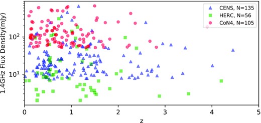
The distribution of three radio data sets. The blue triangles, green squares, and red circles from CENSORS, Hercules, and CoNFIG-4, respectively, are our used sources. Their amounts are listed in the legend.
1.4 GHz flux counts of data sets with z ≥ 0.1.
| Data set | N (F1.4 GHz ≥ 50 mJy) | N (F1.4 GHz ≥ 10 mJy) | N (all) |
|---|---|---|---|
| CENSORS | 25 | 108 | 135 |
| Hercules | 11 | 25 | 56 |
| CoNFIG-4 | 105 | 105 | 1051 |
| Data set | N (F1.4 GHz ≥ 50 mJy) | N (F1.4 GHz ≥ 10 mJy) | N (all) |
|---|---|---|---|
| CENSORS | 25 | 108 | 135 |
| Hercules | 11 | 25 | 56 |
| CoNFIG-4 | 105 | 105 | 1051 |
Note.1CoNFIG-4 data include a sample of z = 0.0963.
To keep samples rich enough, we use CENSORS and Hercules to estimate the BRS z probability density with F1.4 GHz ≥ 10 mJy and all sets to the z density with F1.4 GHz ≥ 50 mJy.
Although our CoNFIG-4 data set contains the original 184 and three extra radio sources, only 105 of them have z ≥ 0.0963. Therefore, we re-scale the sky coverage as 105/187 * 52 ≈ 29.2 deg2, to counteract the lost z information.
3.1.2 New descriptions and one example
Polynomial fitting often has intractable zero-points. Specific fitting models such as gamma require more prior knowledge. And different-length z-bin would lose diverse information in the process.
Consequently, we introduce the KDE to implement a non-parametric fitting of z probability density without bins. Particularly when using a Gaussian kernel, the final distribution can be extracted by multiGaussian fitting. In the next paragraphs, we will show the data process of CoNFIG-4 with F1.4 GHz ≥ 50 mJy as an example. For other data sets following the same procedure, we would give results directly.
The scale of abscissa would affect the profile’s height, so we fix the gap of z as 0.1 at the start.
We use Gaussian kernel KDE (KernelDensity in sklearn) to fit the CoNFIG-4 data (both z and F1.4 GHz). KDE has a key parameter ‘bandwidth’ equivalently controlling the width of a single Gaussian count unit, which replaces a single rectangle count unit in a histogram. Narrower bandwidth remains more features, but leads to a more flexible model and less generalization capability.
For instance, we plot the fitted probability density function (PDF) with several bandwidths in the upper panel of Fig. 4 and show their rms error count from 500 rounds’ eight-fold random-shuffle cross-validation in its lower panel. The mean rms error decreases when the bandwidth diminishes, and the rms error distribution keeps stable. However, the 0.1 bandwidth at least needs a 5-Gaussian profile to fit. Thus, we accept a bandwidth ≥0.2 but as small as possible and always prefer a simpler multiGaussian fitting.
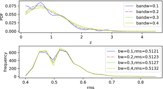
The different bandwidths in CoNFIG-4 KDE. In the upper panel, the blue, red dash–dotted, green dashed, and yellow solid curves are the PDF with bandwidths from 0.1 to 0.4. In the lower panel, four curves are the rms error distribution in 500 rounds’ cross-validation, their colours correspond to the upper, and their mean rms are shown in the legend.
Next, we explore what statistical model covers CoNFIG-4 better. Noticing the denser low-redshift region, we use exponential, gamma, and Weibull distribution to fit the data.
We use Kolmogorov–Smirnov (K–S) test (kstest in scipy) to compare their fittings. If it returns a p value higher than our expected level of significance (α = 0.05), we can regard the two arrays from the same distribution. It shows the p values 0.0815 of the norm and 0.0573 of exponential (exp), while gamma and Weibull both have p values lower than 0.05. But the auto K–S test can not process the KDE curve. Therefore, in manual coding, we plot the cumulative distribution function (CDF) of real 0.1-z-bin data, exponential, KDE curve of bandwidth 0.2 and 0.3 in Fig. 5, and compare the maximum vertical distances (maxVDs) between real data CDF and tested CDF. Now, we define a constant
where α is the significant level and m and n are the numbers of real samples and tested samples, respectively. We gain the KDE profile from real samples, so C(0.05,104,104) ≈ 0.1883. If maxVD is less than the constant C, we can treat the two arrays from the same distribution.
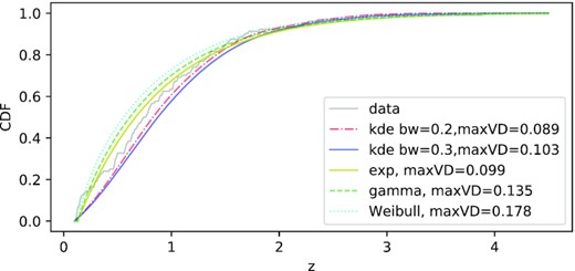
The CDF for manual K–S test. The grey, red dash–dotted, blue, yellow, green dashed, and cyan dotted curves are the CDFs of real data (CoNFIG-4), two KDEs (bw = 0.2, 0.3), exp, gamma, and Weibull, respectively. Their maxVDs are listed in the legend.
From Fig. 5, the exp and two KDEs comparatively fit real data from the aspect of maxVD. We plot their PDFs in Fig. 6, where the exp and two KDEs are distinct. The gamma and Weibull are worse than the exp because their p values are lower than 0.05. Though the exp matches the peak point well, it behaves poorly at the adjacent redshifts, causing the overestimation in our most concerned low-redshift (z< 1) region.
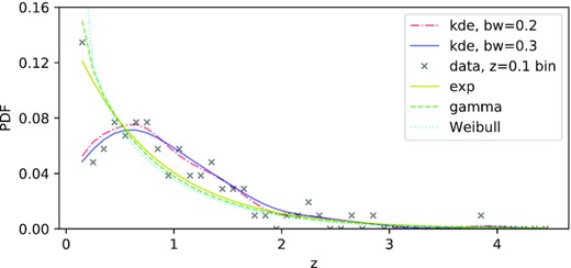
The fitted PDF of CoNFIG-4. The gray cross is the probability density law of the real data. The red dash–dotted, blue, yellow, green dashed, and cyan dotted curves are the PDFs of two KDEs (bw = 0.2, 0.3), exp, gamma, and Weibull, separately.
Finally, multiGaussian fitting exports an analytic expression for the BRS integration in equation (8). To balance the informative feature and simple model, we plot the 0.2-bandwidth fitting in Fig. 7 and choose the 3-Gaussian result.
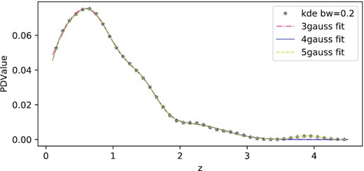
The multiGaussian fitting of KDE with bandwidth 0.2 for CoNFIG-4. The grey star is KDE data. The red dash–dotted, blue, and yellow dashed curves are 3-, 4-, and 5-Gaussian models, separately.
Because we mainly concern with the KDE performance, we will ignore other statistical model fittings hereafter.
3.1.3 Probability density of BRSs
According to the H21A spectroscopic observation (Geréb et al. 2015), where three BRSs in all 32 ones showed F1.4 GHz ≤ 50 mJy (but ≥35 mJy). Thus, 50 mJy can be a proper lower limit for the present observation capability. And we regard 10 mJy as an optimistic capability for the next generation of radio telescopes or arrays.
We make KDE for different radio sets, accumulate with two flux levels (50 and 10 mJy), check with manual K–S test, average them with the weights of their number density per square degree sky (|$\sigma _\mathrm{CO_{50}}$| = 3.5962, |$\sigma _\mathrm{CE_{50}}$| = 4.1667, |$\sigma _\mathrm{HE_{50}}$| = 5.5, |$\sigma _\mathrm{CE_{10}}$| = 18, |$\sigma _\mathrm{HE_{10}}$| = 12.5), and plot these in Fig. 8, where larger bandwidths relate to simpler models, but lose more features, especially merging the first two peaks, which heavily impact our estimation in the low-z region. Therefore, we fix the bandwidth as 0.2.
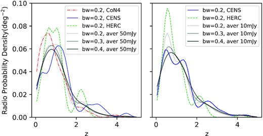
The multiGaussian fitting of the KDE curve with bandwidth 0.2 for all radio data sets. The left panel is for F1.4 GHz ≥ 50 mJy and the right is for F1.4 GHz ≥ 10 mJy. The red dash–dotted, blue, and green dashed curves are the 0.2-bandwidth KDE results of CoNFIG-4, CENSORS, and Hercules, separately. The grey lines are the number-weighted KDEs with different bandwidth components.
We make multiGaussian fitting for a 2-dimension (z-F1.4 GHz) 0.2-bandwidth KDE curves in Fig. 9. The 3-Gaussian is our prioritized option for simplicity. But in the high-z region (z > 4) of the 10 mJy lower limit, it loses the last peak and causes an irreparable decrease compared with the 50 mJy lower limit, even considering the two area number densities. Such inconsistency obliges us to add an extra Gaussian component to solve it, and the final 4-Gaussian fitting parameters and their 1σ errors are given in Table 3.
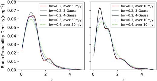
The multiGaussian fitting of averaged 0.2-bandwidth radio KDE curve. The left panel is for F1.4 GHz ≥ 50 mJy and the right is for F1.4 GHz ≥ 10 mJy. The red, grey, and black curves are the KDE averaged result and its KDE (bandwidth = 0.2, 0.3) individually. The blue dashed and green dash–dotted lines are the averaged other bandwidth radio KDEs.
MultiGaussian fitting of averaged 0.2-bandwidth radio KDE curves.
| Component | a1 | μ1 | σ1 |
|---|---|---|---|
| 50 mJy-1 | 0.0579 ± 0.0011 | 0.5790 ± 0.0187 | 0.3930 ± 0.0123 |
| 50 mJy-2 | 0.0395 ± 0.0030 | 1.1939 ± 0.0111 | 0.2711 ± 0.0084 |
| 50 mJy-3 | 0.0124 ± 0.0002 | 2.2123 ± 0.0168 | 0.4869 ± 0.0208 |
| 50 mJy-4 | 0.0012 ± 0.0002 | 4.0000 ± 0.1029 | 0.5000 ± 0.1178 |
| 10 mJy-1 | 0.0706 ± 0.0003 | 0.5193 ± 0.0023 | 0.2788 ± 0.0016 |
| 10 mJy-2 | 0.0447 ± 0.0003 | 1.2491 ± 0.0033 | 0.3031 ± 0.0042 |
| 10 mJy-3 | 0.0127 ± 0.0001 | 2.2949 ± 0.0122 | 0.5049 ± 0.0147 |
| 10 mJy-4 | 0.0015 ± 0.0001 | 4.0488 ± 0.0515 | 0.5000 ± 0.0588 |
Note.1Gaussian function is |$f(z)=\frac{a}{\sqrt{2\pi }\sigma }\exp {[\frac{(z-\mu)^2}{2\sigma ^2}]}$|.
The fourth Gaussian in two KDEs are constrained insufficiently: the a, μ, and σ approach their set borders of 0.15 (a+), 4(μ-), and 0.5 (σ+). If we loosen the borders, the 4-Gaussian tends to become the 3-Gaussian again. Actually, our intention is to derive an approximate KDE expression for numerical integration, and the 4-Gaussian fitting traces the KDE better than the 3-Gaussian, which is enough. Besides, we find that the former three components (eight parameters, excluding σ3) are insensitive to the slight change of limitation (keeping μ4 > 3.5), varying less than 5 per cent (σ3 is 20 per cent) and 10 per cent in the fitted values and errors. Moreover, the curve tails (z > 4) are quite small, only covering less than 1 per cent of the total area under the curve. Therefore, we choose to use the 4-Gaussian.
The errors in Table 3 come from our used samples, and do not reflect the uncertainty including sampling, which need the bootstrap method to convey. The bootstrap randomly re-samples from the original data set (A0) with replacement forming a number of new data sets (|$\mathscr {A}_\mathrm{N}=\lbrace A_\mathrm{i}\rbrace _\mathrm{N}$|, often N ≥ 1000) with the same data volume. One conducts statistical inference from the newly generated sets (|$\mathscr {A}_\mathrm{N}$|) assuming the A0 and |$\mathscr {A}_\mathrm{N}$| from the almost same underlying population. Thus, it provides a more robust 1σ estimation from the potential sample variations, particularly for small sample data.
We re-sample the three radio data sets 10 000 times separately, make number-weighted 0.2-bandwidth KDE, extract its 3σ range in every abscissa (z) point, and plot them in Fig. 10. The bootstrap 1σ errors are more inclusive than the parameter-fluctuation errors in multiGaussian (Table 3), and used by us.
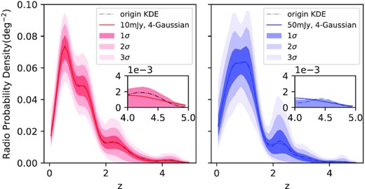
The PDF and 3σ errors of 0.2-bandwidth radio KDE curve. The left panel is for F1.4 GHz ≥ 50 mJy and the right is for F1.4 GHz ≥ 10 mJy. The solid and dash–dotted lines are 4-Gaussian fitted and their original KDE curve. The darkest and lightest areas are the 1σ and 3σ errors respectively. The inserted small panels zoom in their own tails in the high-z region, showing the imperfection of the fourth component.
The above procedure gives the radio source z probability density with different F1.4GHz levels, which needs to multiply with a number density per square degree sky σ to become number density. With number-weighted average from the three data sets, we obtain σ′50 = (1052/29.2 + 252/6 + 112/2)/(105 + 25 + 11) ≈ 3.714 and σ′10 is 16.966. Similar to Allison et al. (2022), we also search the σ in the whole NVSS catalogue with a max radio diameter filter (θ < 60 arcsec) to exclude the extended BRSs, which worsens the covering factor of DLA. Given that the NVSS covers 82 per cent of the entire sky (33830 deg2), we collect N50 mJy = 125525 and N10 mJy = 544130, finally adopting σ50 = 3.71 and σ10 = 16.09 instead of σ′50 and σ′10.
3.2 Forecasting of observed H21As
The recent research of DLA distribution at wide z region (0 ≲ z ≲ 5) was advanced by Rao et al. (2017). They provided an optical MgII pre-selection criterion of DLAs, used it to identify 70 DLAs at low-z region (z ≲ 1.65) from 369 MgII absorbers, and combined many high-z (z ≳ 1.65) SDSS-detected DLAs and a low-z modified value to give a global redshift number density:
Although their result is enough for the z evolution of DLAs, they smoothed out the local DLA distribution features by three wide z bins, which is inadequate for cosmic acceleration observation. So, we use their identified 64 DLAs (NHI > 2 × 1020 cm−2) from 369 MgII absorbers, and miss six DLAs from their full samples. First, Rao, Turnshek & Nestor (2006) presented 41 DLAs from 197 MgII absorbers, while we only find 38 DLAs with |$W_\mathrm{0}^{\lambda 2796}\gt 0.6\mathrm{\mathring{\rm A}}$|. Then, Turnshek et al. (2015) selected 26 DLAs from 96 MgII absorbers, while we just extract 23 DLAs. Neeleman et al. (2016) provided extra 23 DLAs with z and NHI. We plot all 87 DLAs in Fig. 11.

The distribution of 87 DLAs for number density nD. The blue triangles, green squares, and red circles from R06, T15, and R17, separately. The three data sets were all included in R17 article. The yellow pentagons come from N16. Their sample amounts are listed in the legend.
Similarly, we make 2-dimension (z-NHI) KDE for the 87 DLAs with two lower NHI levels, NHI > 2 × 1020 cm−2 (|$\lg N_\mathrm{HI}\gt 20.3$| for visual simplicity, although it should be |$\lg (N_\mathrm{HI}/\mathrm{cm^{-2}})\gt 20.3$|) and NHI > 6.31 × 1020 cm−2 (|$\lg N_\mathrm{HI}\gt 20.8$|), and use manual K–S test to compare the constant C and their maxVDs. Provided the simple profiles of KDE in Fig. 12, we choose a 3-Gaussian fitting with 0.1 bandwidth for accuracy, and list the fitted values and errors in Table 4. A 10 000-bootstrap gives the 1σ errors in Fig. 13.
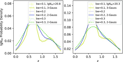
The multiGaussian fittings of KDE curves for 87 DLAs with different bandwidths. The left panel is for |$\lg N_\mathrm{HI}\ge 20.8$| and the right is for |$\lg N_\mathrm{HI}\ge 20.3$|. The thin pale curves are KDE curves with different bandwidths, and the thick dark lines are their fittings, respectively.
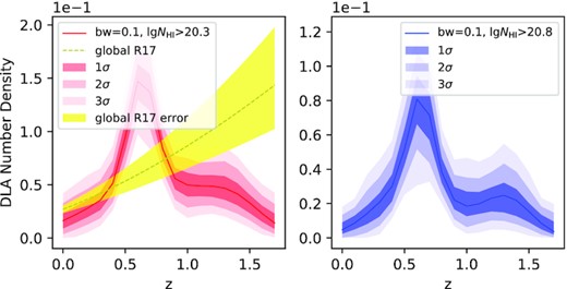
The number distribution and 3σ errors of 87 DLAs. The left panel is for |$\lg N_\mathrm{HI}\ge 20.3$| and the right is for |$\lg N_\mathrm{HI}\ge 20.8$|. The solid lines are their 3-Gaussian fitting of KDE curves, and the coloured areas present the 3σ regions, individually. The yellow dashed line and area in the left panel are the DLA number distribution and error region from R17.
MultiGaussian fitting of 0.1-bandwidth DLA KDE curves.
| Component | a | μ | σ |
|---|---|---|---|
| 20.8–1 | 0.0323 ± 0.0016 | 0.5789 ± 0.0097 | 0.2953 ± 0.0098 |
| 20.8–2 | 0.0517 ± 0.0015 | 0.6350 ± 0.0020 | 0.0993 ± 0.0028 |
| 20.8–3 | 0.0231 ± 0.0006 | 1.3149 ± 0.0084 | 0.2007 ± 0.0077 |
| 20.3–1 | 0.1025 ± 0.0021 | 0.6336 ± 0.0018 | 0.1099 ± 0.0024 |
| 20.3–2 | 0.0509 ± 0.0024 | 0.7506 ± 0.0495 | 0.4782 ± 0.0388 |
| 20.3–3 | 0.0233 ± 0.0059 | 1.3649 ± 0.0197 | 0.2273 ± 0.0315 |
With the 21cm absorption optical depth τ21(ν) = −log {1 − ΔF(ν)/[CfF(ν)]}, NHI can be expressed as (Kanekar et al. 2014)
where TS and Cf is spin temperature and covering factor of DLA, ΔF is the absorbed flux density, and F is the continuum flux density. Because of the low 21cm optical depth (τ21 ≪ 1) for most DLAs, equation (13) can reduce to
NHI is determined by TS, Cf. and integrated per cent absorption. Constraints on NHI can be decomposed into three parts.
However, according to the same article (Kanekar et al. 2014), no statistical relations are found in TS–NHI and TS–Cf, while NHI–∫τ21(ν)dν has a 3.8σ-significance correlation. They find a 37-DLA data set with their z, NHI, estimated TS. and Cf in the foreground of compact radio quasars. Depending on this data set, we will make a 3-dimension KDE in the parameter space of z–NHI–TS, and limit NHI and TS as before. Because the NHI–Cf relation was not explored in their paper, we do not limit Cf together.
Grasha et al. (2020) found the best TS is 175/CfK for low-z (z < 1) DLAs, and 100/Cf–500/CfK is acceptable. Allison (2021) obtained 274 and 576 K in the low-z region (z < 1) in the detection and non-detection situations (2σ). Overall, we take TS of 500 and 1000 K as two limits, with the former two |$\lg N_\mathrm{HI}$| limits (20.3, 20.8) in our estimation of |$\kappa (z,\lg N_\mathrm{HI},T_\mathrm{S})$|.
Again, we plot the extra 37 DLAs in Fig. 14. Making 3-dimension KDE with TS and |$\lg N_\mathrm{HI}$| limits and conducting a manual K–S test, we perform a 3-Gaussian fitting (considering the actual shape of detection rate curves, we use one subtract the 3-Gaussian as the results) with 0.3 bandwidth in Fig. 15 with their parameters listed in Table 5. The less bandwidth and more Gaussians are discarded to alleviate overfitting. The 3σ errors from 10000-bootstrap are offered in Fig. 16. The 20.3–500 situation in Table 5 has the most unsuccessful constraint, reflected by the widest 3σ region in Fig. 16. But considering the good performance between the KDE curve and its multiGaussian fitting, we still accept the results.
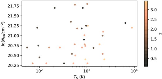
The distribution of 37 DLAs for detection rate κ. The darker sample has a larger redshift.
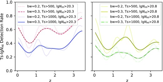
The multiGaussian fittings of KDE curves for 37 DLAs with different bandwidths. The left panel is for |$\lg N_\mathrm{HI}\ge 20.3$| and the right is for |$\lg N_\mathrm{HI}\ge 20.8$|. The thin pale curves are 0.2-bandwidth KDE curves and the thick dark lines are 0.3-bandwidth ones. The unlabelled grey dotted lines are 3-Gaussian fitting for 0.3-bandwidth KDEs.
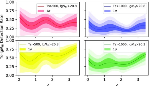
The detection rates and 3σ errors of 37 DLAs. The left panels are for TS > 500 K and the right are for TS > 1000 K. The upper panels are for |$\lg N_\mathrm{HI}\ge 20.8$| and the lower are for |$\lg N_\mathrm{HI}\ge 20.3$|. The solid lines are the 3-Gaussian fitting of KDEs, and the coloured areas present their 3σ errors individually. Only the darkest 1σ regions are labelled in the legends.
MultiGaussian fitting1 of 0.2-bandwidth detection KDE curves.
| Component | a | μ | σ |
|---|---|---|---|
| 20.8-1000-1 | 0.4686 ± 0.1408 | 3.8692 ± 0.1728 | 0.4394 ± 0.0960 |
| 20.8-1000-2 | 0.7740 ± 0.0154 | 2.4748 ± 0.0154 | 0.8251 ± 0.0534 |
| 20.8-1000-3 | 0.7309 ± 0.0174 | 0.5183 ± 0.0324 | 0.7968 ± 0.0282 |
| 20.3-1000-1 | 0.5850 ± 0.0084 | 3.6992 ± 0.1645 | 1.6574 ± 0.2301 |
| 20.3-1000-2 | 0.2529 ± 0.0285 | 2.3546 ± 0.0097 | 0.4074 ± 0.0180 |
| 20.3-1000-3 | 0.5783 ± 0.0499 | 0.6383 ± 0.0187 | 0.6637 ± 0.0254 |
| 20.8-500-1 | 0.1109 ± 0.0156 | 2.4000 ± 0.0280 | 0.5282 ± 0.0506 |
| 20.8-500-2 | 0.1890 ± 0.0304 | 0.4603 ± 0.0331 | 0.3654 ± 0.0380 |
| 20.8-500-3 | 0.6210 ± 0.0126 | 1.5104 ± 0.1410 | 2.0000 ± 0.1354 |
| 20.3-500-1 | 0.2378 ± 1.1207 | 0.0602 ± 3.4411 | 0.5034 ± 2.3483 |
| 20.3-500-2 | 0.4541 ± 0.0020 | 2.2745 ± 0.0136 | 0.9268 ± 0.0163 |
| 20.3-500-3 | 0.3842 ± 2.2242 | 0.6983 ± 0.7163 | 0.4088 ± 0.2259 |
Note.1The actual curve of detection rate is the result that one subtracts the 3-Gaussian fitting.
3.3 Anticipation of potential H21As
Given all the components, we can calculate the potential H21As number density [equation (8)] in Fig. 17 and its integrated number count in Fig. 18 from z = 0.1 to eliminate the objects in the local Universe.
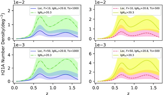
The potential H21A number density. The left panels are for TS > 1000 K and the right are for TS > 500 K. The upper panels are for F1.4 GHz > 10 mJy and the lower are for F1.4 GHz > 50 mJy. The lines and corresponding colour areas are their density curves and 1σ errors.
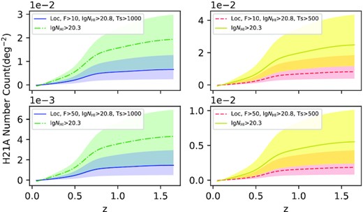
The potential H21A number count. The left panels are for TS > 1000 K and the right are for TS > 500 K. The upper panels are for F1.4 GHz > 10 mJy and the lower are for F1.4 GHz > 50mJy. The lines and corresponding colour areas are their count curves and 1σ errors.
FAST covers about 24000 deg2 (Li et al. 2018) and the redshift of 0 to 0.352 (1050–1450 MHz). ASKAP covers 33000 deg2 (Allison et al. 2022) and the redshift of 0.4 to 1.0 (711.5–999.5 MHz). As for the most remarkable instrument, the SKA1M covers about 30 000 deg2 (Kloeckner et al. 2015; Weltman et al. 2020) and the redshift of 0 to 1. We list the predicted detection yield in Table 6 for each instrument and lower limit condition, and the 1σ errors are multiplicative result from the three-component bootstraps.
The detection yield of potential H21As in each condition.
| Telescope | Fmin/mJy | |$\lg (N_\mathrm{HI,min}$|/cm−2) | TS,min/K | Prediction |
|---|---|---|---|---|
| FAST | >50 | >20.8 | >1000 | |$5.8^{+5.2}_{-4.2}$| |
| >500 | |$6.6^{+9.4}_{-4.0}$| | |||
| >20.3 | >1000 | |$16.0^{+8.3}_{-11.4}$| | ||
| >500 | |$18.7^{+17.8}_{-9.8}$| | |||
| FAST | >10 | >20.8 | >1000 | |$26.2^{+21.4}_{-18.6}$| |
| >500 | |$30.0^{+39.4}_{-17.2}$| | |||
| >20.3 | >1000 | |$72.1^{+33.3}_{-49.7}$| | ||
| >500 | |$84.7^{+73.2}_{-46.0}$| | |||
| ASKAP | >50 | >20.8 | >1000 | |$31.5^{+32.2}_{-19.6}$| |
| >500 | |$39.8^{+52.7}_{-20.8}$| | |||
| >20.3 | >1000 | |$90.7^{+56.1}_{-57.8}$| | ||
| >500 | |$116.5^{+96.6}_{-63.0}$| | |||
| ASKAP | >10 | >20.8 | >1000 | |$137.2^{+129.8}_{-81.1}$| |
| >500 | |$172.8^{+214.7}_{-83.6}$| | |||
| >20.3 | >1000 | |$394.2^{+220.6}_{-250.1}$| | ||
| >500 | |$506.7^{+385.6}_{-255.3}$| | |||
| SKA1M | >50 | >20.8 | >1000 | |$37.8^{+37.1}_{-24.8}$| |
| >500 | |$46.6^{+62.3}_{-25.1}$| | |||
| >20.3 | >1000 | |$107.0^{+63.7}_{-69.9}$| | ||
| >500 | |$135.0^{+114.7}_{-73.9}$| | |||
| SKA1M | >10 | >20.8 | >1000 | |$165.8^{+150.2}_{-102.5}$| |
| >500 | |$204.2^{+255.3}_{-102.7}$| | |||
| >20.3 | >1000 | |$469.2^{+250.4}_{-293.8}$| | ||
| >500 | |$591.7^{+461.7}_{-302.9}$| |
4 DISCUSSION
We emphasize that the S–L signal is a direct measurement, and its theoretical derivation is independent of Einstein’s equation and Copernican principle (Yu et al. 2014), compared with other common cosmological probes like SNe Ia. But the different matter structures of every sightline in the signal propagation necessitates further studies of the inhomogeneity influence on the S–L signal.
The systematics of the S–L effect mainly contains two parts. First, the proper acceleration of the observer involves the earthly, solar, galactic, and cosmological frames. The former two terms can be calculated in the highest level of cm s−1 (one-decade accumulation of S–L signal) (Wright & Eastman 2014). The solar revolution around the galactic centre can be accurately measured by pulsar timing (Zakamska & Tremaine 2005), Gaia Data Release 3 (Gaia Collaboration 2021) and very long baseline interferometry (VLBI) (Xu, Wang & Zhao 2012; Titov & Krásná 2018) in mm s−1 yr−1 level, which is the same as S–L signal. And the proper motion of extragalaxies is accessible by VLBI (Titov, Lambert & Gontier 2011; Titov et al. 2022). The possible redshift uncertainties were given in Bolejko, Wang & Lewis (2019) and reviewed in Lu et al. (2022). Second, the peculiar motion of absorption line systems would impact the S–L signal. Combining the various physical conditions of DLAs (Dutta et al. 2017), the neutral mass (NM) ratio (cold NM:unstable NM:warm NM = 28:20:52) in our galaxy (Murray et al. 2018), and fig. 14 from Kanekar et al. (2014), there do exist some DLAs with sharp absorptions as ideal targets for probing S–L signal. Additionally, the data process introduces new uncertainty when signal extraction and flux calibration. It is not the primary challenge but needs to maintain the same procedure and reform with new techniques.
Though simple statistical models like exponential can determine the number densities, and KDE would decrease generalization ability. We still use KDE for some reasons, most importantly to keep the method consistent in the data process. Second, as a non-parametric estimation, KDE needs less prior knowledge about the realistic distribution. Third, these simple-peak models are inadequate for multipeak distribution. Fourth, when filtering data with different lower limits, some samples are discarded but close to the limits. However, KDE will record the contributions of these border-near samples. Although KDE is a sensitive method suffering more fluctuations from many factors, it provides similar features (a big bulge containing two peaks and a small bulge/peak) in the two panels of Fig. 10, proving its robustness sufficiently.
The multiGaussian fittings for two components of KDEs in Tables 3 and 5 offer poor constraints, but the fittings quite approach the KDEs and such a defect does not hinder our estimation.
Most used radio samples are radio-loud AGNs, but other information such as morphological and spectral types was not recorded. One can better grip their redshift distribution and radio luminosity function by dividing samples into more sub-types if acquiring more data, but now they are beyond our present reach.
With different radio data sets, it is necessary to compare their observations. The radio sources in CENSORS and Hercules were preliminarily selected by pioneering radio mapping, and then probed by subsequent optical spectra. Original CENSORS (Brookes et al. 2008) optically observed 143 in all 150 sources, providing a 71 per cent spectroscopic completeness. As for the rest, the K-z (and I-z for one source) relation was used to estimate their redshifts. Original Hercules (Waddington et al. 2001) with 72 sources, offered 47 spectroscopic redshifts, found 10 upper limits of redshift from the literature, and estimated the broad-band photometric redshifts for the rest. Rigby et al. (2011) rearranged the two sets with some published reassessments. They selected a 135-sample subset for CENSORS with 73 per cent spectroscopic completeness, and a 64-sample subset for Hercules with 40 spectroscopic and 20 photometric redshifts. As for CoNFIG-4 samples (Gendre & Wall 2009; Gendre et al. 2010), they were selected from NVSS and FIRST (White et al. 1997) counterplots with complete Fanaroff–Riley morphology, and reviewed for their optical information. No observation was performed in CoNFIG papers, hence their redshift information was all from literature. For the samples without redshifts in CoNFIG-4, they have roughly similar but lower flux distribution compared with redshift ‘owners’ in Fig. 19, so it is hard to regard them as statistically less luminous in F1.4 GHz. But we find that most samples without redshifts do not have SDSS magnitudes recorded in the original data.
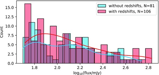
The histogram of CoNFIG-4 data for F1.4GHz. The blue bars are for the samples without redshifts, and the blue line is their KDE curve, while the red ones are for those redshift ‘owners’.
Optical selections inserted in observation unavoidably bias radio number density, but more data sets can provide a more robust prediction than a single one. Like the radio source number density per square degree sky (σ) at the end of Section 3.1.3, only with three data sets, our estimated σ50′ = 3.714 can approach the NVSS value σ50 = 3.71, while any single set corresponds a greater deviation.
Rao et al. (2017) provided abundant DLAs at low redshift (z ≲ 1.65) where the ground-based optical telescope can not directly observe. A reasonable speculation is that their pre-selection is biased by luminosity and dust extinction, having the risk of omitting some MgII absorbers, DLAs without MgII absorption, and deriving biasedly higher ΩDLA. However, they found (in Section 4 of that article) no evidence for these effects at z < 1.65. And Kanekar’s conclusion (Kanekar et al. 2014) also disapproves of this selection effect in the aspect of TS distributions.
We notice that Dutta et al. (2017); Dutta (2019) advanced an absorption-blind or galaxy-selected approach, selecting a galaxy visually close to a background quasar (Quasar–Galaxy Pair, QGP) without the prior of any absorption toward the quasar. Their method is not intuitively biased as MgII pre-selection. We hope their project finds more QGPs for the distribution of radio DLASs.
In addition to Rao’s and Neeleman’s I-type DLAs, there exist other DLA data sets, e.g. Curran et al. (2016); Curran (2021). Curran’s data provide 85 A-type and 56 I-type DLAs with z > 0.1. Although Curran’s data cover wider redshift and more samples, they are collected from different observations. The decisive reason for discarding Curran’s data is they do not contain NHI, which is included in Rao’s data, and we want to use 2-dimension (z and NHI) KDE for more features. Moreover, we plot Curran’s and Rao’s data in Fig. 20, and Rao’s KDE profile of I-type DLAs almost envelopes Curran’s, exceptionally raising a bulge mainly because of the subset T15 (Turnshek et al. 2015) with z from 0.4 to 1.0. Besides, it is normal that total Curran’s KDE profile covers Rao’s, because the former contains extra A-type DLAs, which are not suitable for S–L signal. Because over half DLAs (28 in 41) overlap Rao’s samples, we do not plot Neeleman’s KDE.
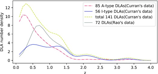
The KDE fittings (bandwidth = 0.2) of two DLA data sets. The grey and yellow dashed curves are for the total two sets. The red dash–dotted and blue curves are the A- and I-type DLAs in Curran’s data, separately.
The different tendencies in the low-z region between our KDE-derived and Rao’s DLA number density in the left panel of Fig. 13, apart from their wide z-bin, are mainly caused by Rao’s modified DLA number density values at z = 0 (Zwaan et al. 2005; Braun 2012). The modification is reasonable if we consider the left end of Curran’s I-type KDE, which is slightly higher than Rao’s in Fig. 20, indicating the low-z shortage of Rao’s samples. But the single value point nDLA(z = 0) can not change the KDE result unless we have real low-redshift DLAs to feed the algorithm.
Our NHI–TS constraints for DLAs and the H21A-to-DLA proportional constant η, mainly rely on the 37-DLA data from Kanekar et al. (2014). Hence our results are inevitably affected by small samples and Poisson errors, and need more ‘full’ information (z, NHI, TS, and Cf) DLAs to overcome.
The recent study of DLAs detection yield includes the remarkable work from Allison et al. (2022), where they defined a completeness function |$\mathscr {C}$| with the 1000 mock spectra recovered from FLASH early survey of the GAMA 23 field (Allison et al. 2020), and used an NHI frequency distribution function |$\mathscr {F}$| linearly interpolated from z = 0 (Zwaan et al. 2005) and z > 2 (Bird et al. 2017), to predict the number of I-type and A-type DLAs in the ASKAP range. Future researchers will be enlightened to improve their NHI frequency distribution. And their completeness function reminds us that more factors, such as signal-to-noise rate and blind-survey resolution (related to H21A’s line width distribution), can be considered in prediction. These observational limitations from specific facilities are more concrete, and entail our further efforts.
An interesting difference between our prediction and the Allison’s of ASKAP is, in our 37 DLAs, the low-NHI I-type ones are more than the high-NHI. Namely, our higher sensitivity condition in NHI (to discover more DLAs) is to lower NHI, while they need to increase it. Their complicated functions |$\mathscr {C}$| and |$\mathscr {F}$|, both relate to NHI, and both are not plotted with respect to NHI. Thus, it is hard to say which one (|$\mathscr {C}$| or |$\mathscr {F}$|) dominates this difference.
Given more physical constraints to potential intervening H21As for FAST, our most optimistic expectation is quite small (80), around 1 or 2 order magnitude smaller than some previous work, such as 1500 (Zhang et al. 2021) from a local luminosity function estimation and 2600 (Jiao et al. 2020) for a decade CRAFTS observation (Zhang et al. 2019) with a simpler integration of equation (8). However, our optimistic result approaches the magnitude of 100 from ALFALFA-survey estimation (Wu et al. 2015). Additionally, Zhang’s 1500 result may omit that only about 10 per cent AGNs are radio-loud and ignored AGN’s z distribution.
5 CONCLUSION
In this paper, we make a small but important distinction between the global and dynamical |$\ddot{a}$| and the local and observed |$\dot{v}_\mathrm{S}$| at first, and emphasize that only the |$\ddot{a}$| can express an actual expansion state for the whole Universe at one certain time, but it has not been measured model-independently.
Subsequently, in the bulk of the paper, we separately explore (i) nR, the radio-source redshift number density per square degree via three data sets (with z and F1.4GHz), (ii) nD, the DLA redshift number density in the sightline through 87 DLAs from two low-redshift (z ≲ 1.65) data sets (with z, NHI), and (iii) κ, the DLA detection rate at given NHI–TS limitations from an extra 37-DLA data set and η (the fraction of H21As in DLAs). (1) Introducing the KDE method, we replace the traditional description of the nR and nD, and propose a data-based κ function, with multiGaussian profiles (Tables 3, 4, and 5) of KDE curves. (2) Adopting the bootstrap method, we give the former three functions 1σ errors (Figs. 10, 13, and 16). (3) We predict the potential blind-survey detection amounts (Table 6) for H21As with various limitations. At most optimistic conditions, FAST covers 80 H21As, ASKAP covers 500, and SKA1M covers 600. Although our results are predicted H21A amount, it is convenient to turn them into DLA amount by dividing the proportional constant η = 0.62.
The lack of BRS and DLA samples with ‘full’ information is one of the crucial obstructions to our study. Nevertheless, with more potential H21As discovered in the future, it is a good chance to research H21As’ physical essences and environments, as well as to revise the BRSs from a new aspect. And all this progress can propel our knowledge of the Universe, and help us to comprehend its expansion history and the underlying drivers.
Acknowledgement
The authors thank the anonymous referee for the kind comments that help us greatly to improve this paper. The authors acknowledge support from National SKA Program of China (2022SKA0110202) and National Natural Science Foundation of China (grants No. 61802428, 11929301).
DATA AVAILABILITY
The data we used in this paper are all open on the Internet. Three radio data sets (Gendre et al. 2010; Rigby et al. 2011) and three DLA data sets (Rao et al. 2006; Turnshek et al. 2015; Rao et al. 2017,) are available in VizieR. The rest DLAs from Kanekar et al. (2014); Curran et al. (2016); Neeleman et al. (2016); and Curran (2021) are directly extracted from their articles.
