


ABSTRACT
We study the formation and early evolution of young stellar objects (YSOs) using three-dimensional non-ideal magnetohydrodynamic (MHD) simulations to investigate the effect of cosmic ray ionization rate and dust fraction (or amount of dust grains) on circumstellar disc formation. Our simulations show that a higher cosmic ray ionization rate and a lower dust fraction lead to (i) a smaller magnetic resistivity of ambipolar diffusion, (ii) a smaller disc size and mass, and (iii) an earlier timing of outflow formation and a greater angular momentum of the outflow. In particular, at a high cosmic ray ionization rate, the discs formed early in the simulation are dispersed by magnetic braking on a time-scale of about 104 yr. Our results suggest that the cosmic ray ionization rate has particularly a large impact on the formation and evolution of discs, while the impact of the dust fraction is not significant.
1 INTRODUCTION
Molecular cloud cores, which are the parent bodies of protostars and protostellar discs, are strongly magnetized (Troland & Crutcher 2008; Crutcher et al. 2010; Crutcher 2012). For example, molecular cloud cores typically have a mass-to-magnetic-flux ratio of 2.0, as revealed by the Zeeman effect (Troland & Crutcher 2008).
Such a strong magnetic field removes angular momentum from the central region (known as magnetic braking) and suppresses disc formation. For example, Basu & Mouschovias (1994) shows that magnetic braking causes an exponential decrease in angular velocity. The molecular cloud core is composed of weakly ionized gases (Umebayashi & Nakano 1990; Nakano, Nishi & Umebayashi 2002; Inoue & Inutsuka 2012). Therefore, non-ideal magnetohydrodynamics (MHD) effects (the Ohmic dissipation, ambipolar diffusion, and Hall effect) that determine the coupling rate between the magnetic field and gas are important. Machida, Inutsuka & Matsumoto (2011), Tsukamoto et al. (2015a), and Tomida et al. (2013) showed that the Ohmic dissipation enables the formation of protoplanetary discs as large as 1 au at the protostar formation epoch by eliminating the coupling between the magnetic field and gas in the first core (Larson 1969). The ambipolar diffusion decouples the magnetic field and gas even at lower densities than the Ohmic dissipation, removing magnetic fluxes from the disc and suppressing the magnetic braking over a wider density range (Mouschovias & Morton 1991; Dapp, Basu & Kunz 2012; Tomida, Okuzumi & Machida 2015; Tsukamoto et al. 2015b; Marchand et al. 2016; Masson et al. 2016; Wurster, Price & Bate 2016; Zhao et al. 2016; Tsukamoto, Okuzumi & Kataoka 2017; Zhao et al. 2018; Wurster, Bate & Bonnell 2021). Therefore, ambipolar diffusion is considered to play a major role in the evolution of magnetic fluxes at standard metal (or dust) fractions and cosmic ray ionization rates.
According to observations, different galaxies and star-forming regions have different cosmic ray ionization rates and metallicities. Previous studies (Padovani et al 2009,2013;Phan, Morlino & Gabici 2018; Williams et al 1998; Caselli et al. 1998) showed that the cosmic ray ionization rate decreases with increasing column density in the molecular cloud (see Padovani et al. (2020) for the review of the cosmic ray propagation in the protostar). Furthermore, Cioni (2009) has found that the metallicity is up to 10 times lower in the Large Magellanic Cloud, Small Magellanic Cloud, and M33 galaxies.
The cosmic ray ionization and dust grains (the amount of which is proportional to the metallicity) act as sources and sinks of charged particles, respectively, and affect the ionization degree of the gas. Therefore, the ionization degree will be high in an environment with high cosmic ray ionization and/or low metallicity. Since non-ideal MHD effects are weaker in gases with a high ionization degree, it is expected that the magnetic braking will be more efficient and that disc formation and its growth will be suppressed. This may be related to the observation by Yasui et al. (2010) that the lifetime of circumstellar discs is shortened in low-metallicity environments.
On the other hand, theory shows that in highly ionized environments, the gas is well coupled to the magnetic field and the angular momentum is removed by magnetic braking, thus preventing the formation of discs. For example, Wurster, Bate & Price (2018a, b), and Kuffmeier, Zhao & Caselli (2020) were inspired by observations of differences in cosmic ray intensity in different star-forming regions to study the effect of cosmic ray ionization rates on disc formation. They found that discs formed in environments with low cosmic ray ionization rates, while discs did not form in environments with high cosmic ray ionization rates, a dramatic change. However, because the effect of metallicity (or dust fraction) was not covered in their study, the effects of metallicity on the evolution of YSOs, including the evolution of discs, have not yet been fully clarified.
As the first step of a series of future studies, we investigate the effect of dust fraction (or amount of dust grains) and cosmic ray ionization rate on the formation and evolution of YSOs using 3D non-ideal MHD simulations.
2 NUMERICAL METHOD AND INITIAL CONDITION
2.1 Numerical method
We solved non-ideal MHD equations,
where ρ is the gas density, P is gas pressure, |$\mathbf {B}$| is magnetic field, Φ is the gravitational potential, and G is a gravitational constant. |$\hat{\mathbf {B}}$| is defined as |$\hat{\mathbf {B}}\equiv \mathbf {B}/|\mathbf {B}|$|. ηO and ηA are the resistivities for the Ohmic dissipation and ambipolar diffusion, respectively. We used a barotropic equation of state in which gas pressure only depends on density. cs, iso = 190 m s−1 is isothermal sound velocity at 10 K. We used a critical density of ρcrit = 4 × 10⁻¹⁴ g cm−3, above which gas behaves adiabatically. In this study, we ignored the Hall effect because the calculation cost was enormous.
We used the smoothed particle magnetohydrodynamics (SPMHD) method to solve the equations (Iwasaki & Inutsuka 2011, 2013). See Tsukamoto et al. (2020) for details on numerical calculations.
To avoid small time-stepping, we employed the sink particle technique (Bate, Bonnell & Price 1995). The sink particle is dynamically introduced when the density exceeds ρsink = 4 × 10⁻¹³ g cm−3. The sink particle absorbs SPH particles with ρ > ρsink within r < rsink = 1 au, and the mass and linear momentum of SPH particles are added to those of sink particles.
2.2 Initial conditions
We used the density-enhanced Bonnor–Ebert sphere surrounded by medium with a steep density profile of ρ ∝ r−4 as the initial density profile, which is the same as our previous studies (Tsukamoto, Machida & Inutsuka 2021),
and
where ρBE is the non-dimensional density profile of the critical Bonnor–Ebert sphere, f is a numerical factor related to the strength of gravity, and Rc = 6.45a is the radius of the cloud core. f = 1 corresponds to the critical Bonnor–Ebert sphere, and the core with f > 1 is gravitationally unstable. A Bonnor–Ebert sphere is determined by specifying the central density ρ0, the ratio of the central density to the density at Rc ρ0/ρ(Rc) and f. In this study, we used the values of ρ0 = 7.3 × 10⁻¹⁸ g cm−3, ρ0/ρ(Rc) = 14, and f = 2.1. Then, the radius of the core is Rc = 4.8 × 10³ au, and the enclosed mass within Rc is |$M_{\rm c}=1 \, {\rm M}_{\odot }$|. The thermal energy of the central core (without surrounding medium) is denoted by the terms Etherm and Egrav, respectively. The αtherm (≡ Etherm/Egrav) is equal to 0.4. The steep envelope was used in order to place the outer boundary far from the cloud core’s centre. With the steep profile, the total mass of the entire domain remains ∼2Mc. For rotation of the cloud core, we used an angular velocity profile of |$\Omega (d)=\frac{\Omega _0 }{\exp (10(d/(1.5 R_{\rm c}))-1)+1}$|, where |$d=\sqrt{x^2+y^2}$| and Ω0 = 2.3 × 10⁻¹³ s−1. Ω(d) is almost constant for d < 1.5Rc and rapidly decreases for d > 1.5Rc. The rotating energy of the core, denoted by Erot, has a ratio to gravitational energy βrot(≡ Erot/Egrav) equals 0.03.
The magnetic field profile has only the z component. The magnetic field strength and plasma β at the centre were B0 = 62 |$\mu$|G and β = 1.6 × 101, respectively. The mass-to-flux ratio of the core μ relative to the critical value was μ/μcrit = (Mc/Φmag) = 3, where Φmag is the magnetic flux of the core and μcrit = (0.53/3|$\pi$|)(5/G)1/2. We resolved 1 |$\, {\rm M}_{\odot }$| with 3 × 10⁶ SPH particles. Thus, each particle has a mass of |$m=3.3\times 10^{-7} \,{\rm M}_{\odot }$|.
The model names and corresponding dust sizes are summarized in Table 1.
Model name, dust fraction, the strength of cosmic ray, and dust model are given.
| Model name | f | |$\zeta _{\rm CR}[\rm {s}^{-1}]$| | Dust model |
|---|---|---|---|
| model_MRN_f1e2_zeta1e17 | 10−2 | 10−17 | MRN |
| model_MRN_f1e3_zeta1e17 | 10−3 | 10−17 | MRN |
| model_MRN_f1e2_zeta1e16 | 10−2 | 10−16 | MRN |
| model_MRN_f1e3_zeta1e16 | 10−3 | 10−16 | MRN |
| Model name | f | |$\zeta _{\rm CR}[\rm {s}^{-1}]$| | Dust model |
|---|---|---|---|
| model_MRN_f1e2_zeta1e17 | 10−2 | 10−17 | MRN |
| model_MRN_f1e3_zeta1e17 | 10−3 | 10−17 | MRN |
| model_MRN_f1e2_zeta1e16 | 10−2 | 10−16 | MRN |
| model_MRN_f1e3_zeta1e16 | 10−3 | 10−16 | MRN |
2.3 Resistivity
In this study, we choose dust fraction and cosmic ray ionization rate as parameters. Then, the resistivity was calculated by chemical reaction calculations with the parameters. See Tsukamoto et al. (2020) for details on chemical reaction network calculation.
For the dust models, we considered a dust size distribution of n(a) ∝ a−3.5 with minimum and maximum dust sizes of |$a_{\min}=0.005 \,\mu {\rm m}$| and |$a_{\max}=0.25 \, \mu {\rm m}$| (MRN distribution). The dust internal density is fixed to be ρd = 2 g cm−3. The dust-to-gas mass ratio f is 10−2 or 10−3 and f = 10−2 is the solar dust-to-gas ratio.
The model names and corresponding dust fraction and cosmic ray ionization rate are summarized in Table 1.
3 RESULTS
3.1 Impact on magnetic resistivity
First, we examine how resistivity depends on cosmic ray ionization rate and dust fraction.
Fig. 1 shows the Ohmic resistivity ηO and ambipolar resistivity ηA with different cosmic ray ionization rates and dust fractions. The left side of Fig. 1 shows ηA (solid line) and ηO (dashed line) as functions of density with a fixed magnetic field strength of |$\mathbf {B}= 3\times 10^{-2} \, \rm {G}$|. The black dotted line is |$\eta _{\rm A} = B^2/(4\pi \gamma \rho C \sqrt{\rho })$| (Shu 1983), where we use |$\gamma = 3.5 \times 10^{13} \,{\rm cm}^3\,{\rm g}^{-1}\,{\rm s}^{-1}$| and |$C=3.0 \times 10^{-16}\,{\rm g}\,{\rm cm}^{-3}$|. In the low-density region (≲10−14 g cm−3), ηA decreases with increasing density. In this density region, gases are ionized by a cosmic ray. Thus, the fraction of the charged particle increases, and ηA decreases. In the intermediate density region (10−14 g cm−3 ≲ ρ ≲ 10−11 g cm−3), ηA increases with increasing density. As the density increases, charged particles are absorbed by dust grains due to the increasing collision rate between dust grains and charged particles. This absorption reduces the number of charged particles and lowers the conductivity. Thus, ηA increases in the intermediate density. In the high-density region (≳10−11 g cm−3), ηA decreases with increasing density.
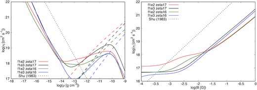
The left-hand panel shows ηA (solid lines) and ηO (dashed lines) as a function of density with a fixed magnetic field strength of B = 30 mG. The right-hand panel shows ηA as a function of the magnetic field with a fixed density ρ = 4 × 10-15 g cm−3. The dotted black line shows |$\eta _{\rm A} = B^2/(4\pi \gamma \rho C\sqrt{\rho })$| given by Shu (1983). We defined γ = 3.5 × 1013 cm3 g−1 s−1 and C = 3.0 × 10⁻¹⁶ g cm−3.
Note that the resistivity decreases with increasing cosmic ray intensity. For example, for ρ ∼ 10−13 g cm−3, model_MRN_f1e2_zeta1e16 has a twice lower ηA than model_MRN_f1e2_zeta1e17 and model_MRN_f1e3_zeta1e16 has an order of magnitude lower ηA than model_MRN_f1e3_zeta1e17. Because cosmic rays ionize neutral gas, clouds have a higher ionization degree when the rays are stronger. As a result, the clouds have higher conductivities and lower ηA.
This indicates that ηA is affected by an increase in cosmic ray intensity and a decrease in dust fraction (solid line). Also, ηA steepens with decreasing dust fraction in the density region (10−14 g cm−3 ≲ ρ ≲ 10−10 g cm−3).
On the other hand, as cosmic rays and dust fraction increase, ηO decreases in the density region (10−12 g cm−3 ≲ ρ ≲ 10−9 g cm−3).
The right-hand panel of Fig. 1 shows ηA as a function of magnetic field at ρ = 4 × 10⁻¹⁵ g cm−3. For all models, the dependence of ηA in a strong magnetic field (≳3 × 10⁻² G) is ηA ∝ B2 as stated by (Shu 1983). In weak magnetic fields, on the other hand, the magnetic field dependence of ηA is not simple. In all models, at least for B < 10−3 G, it is almost independent of the magnetic field, and the relation ηA ∝ B2 is not necessarily true in the region 10−3 G < B < 3 × 10⁻² G.
3.2 Time evolution of models in higher cosmic ray ionization and lower dust fraction environment
In this section, we describe the time evolution of the disc and outflow of each model.
Fig. 2 shows the density evolution on the x–y plane in the 250 au scale box of model_MRN_f1e2_zeta1e17 (top), model_MRN_f1e3_zeta1e17 (second row), model_MRN_f1e2_zeta1e16 (third row), and model_MRN_f1e3_zeta1e16 (bottom), at t = 4.3 × 10⁴ yr (left column), t = 4.7 × 10⁴ yr (middle column), and t = 4.9 × 10⁴ yr (right column). The circumstellar disc is the central high-density region (ρ ≳ 10−14 g cm−3). The disc is formed at t = 4.3 × 10⁴ yr (left column) and is of similar size in all models. At t = 4.7 × 10⁴ yr (middle column), the disc in model_MRN_f1e3_zeta1e16 is smaller than other discs. At t = 4.9 × 10⁴ yr (right column), model_MRN_f1e2_zeta1e17 and model_MRN_f1e3_zeta1e17 maintain the disc. On the other hand, the discs shrink in model_MRN_f1e2_zeta1e16 and model_MRN_f1e3_zeta1e16. A more quantitative analysis of the disc size evolution is presented in Section 3.3.
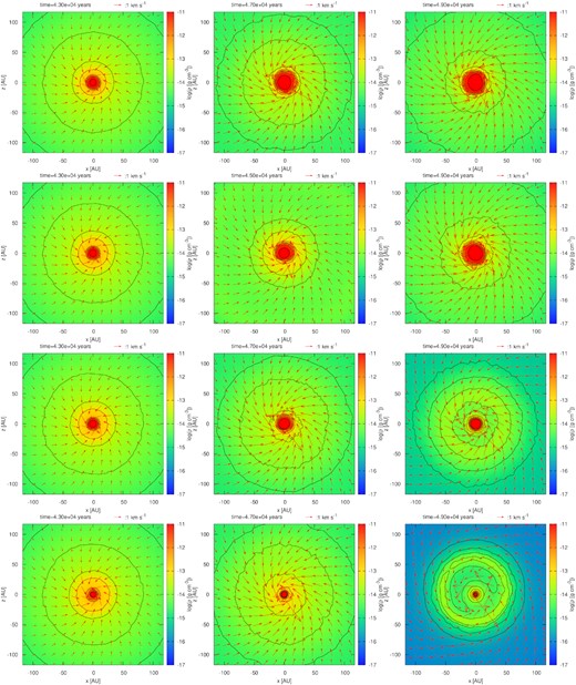
Density maps in two dimensions on the x–y plane for model_MRN_f1e2_zeta1e17 (top), model_MRN_f1e3_zeta1e17 (second row), model_MRN_f1e2_zeta1e16 (third row), and model_MRN_f1e3_zeta1e16 (bottom). The elapsed times are t = 4.3 × 10⁴ yr (left), t = 4.7 × 10⁴ yr (middle), and t = 4.9 × 10⁴ yr (right). Red arrows show the velocity field.
Fig. 3 shows the density evolution on the x–z plane in the 4000 au scale box of model_MRN_f1e2_zeta1e17 (top), model_MRN_f1e3_zeta1e17 (second row), model_MRN_f1e2_zeta1e16 (third row), and model_MRN_f1e3_zeta1e16 (bottom) for the same time period as Fig. 2. All models formed the outflow in our simulation. With high cosmic ray ionization (model_MRN_f1e2_zeta1e16, model_MRN_f1e3_zeta1e16), the outflow reaches further and the outflow velocity is faster than with lower cosmic ray (model_MRN_f1e2_zeta1e17, model_MRN_f1e3_zeta1e17). While focusing on the difference in dust fractions, outflows have a large difference only when |$\zeta =10^{-16} \, \rm {s^{-1}}$|. Section 3.5 contains a more quantitative analysis of the disc size evolution.
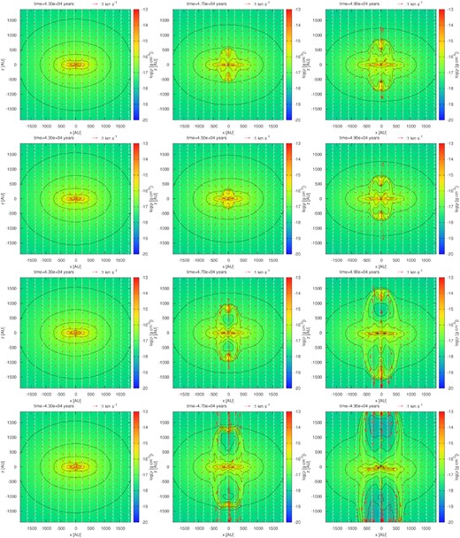
Density maps in two dimensions on the x–z plane for model_MRN_f1e2_zeta1e17 (top), model_MRN_f1e3_zeta1e17 (second row), model_MRN_f1e2_zeta1e16 (third row), and model_MRN_f1e3_zeta1e16 (bottom). The elapsed times are t = 4.3 × 10⁴ yr (left), t = 4.7 × 10⁴ yr (middle), and t = 4.9 × 10⁴ yr (right). Red arrows show the velocity field, and white arrows show the direction of the magnetic field.
3.3 Time evolution of specific angular momentum and disc radius
Here we examine the time evolution of the angular momentum and centrifugal radius in the central region to quantitatively discuss the disc size evolution after protostar formation. The angular momentum of the disc J(ρdisc) is calculated by
For the density threshold of the disc, we use ρdisc = 1.0 × 10⁻¹⁴ g cm−3. At the first output after the sink particle is introduced, the centrifugal radius is calculated by
Here |$\bar {j}(\rho _{\rm disc}) = J(\rho _{\rm disc})/M(\rho _{\rm disc})$|, where M(ρdisc) is the enclosed mass within the region ρ > ρdisc. We regard this centrifugal radius as a disc radius.
The solid line in Fig. 4 shows the time evolution of the centrifugal radius. In low cosmic ray ionization models (red and black lines), the disc continues to grow with time after disc formation (t ∼ 4.3 × 10⁴ yr) and until the end of the simulation (t ∼ 5.2 × 10⁴ yr). Even in models with high cosmic ray ionization (orange and yellow lines), the disc forms at t ∼ 4.3 × 10⁴ yr. However, the disc size does not monotonically increase with time and eventually disappears at the end of the simulation.
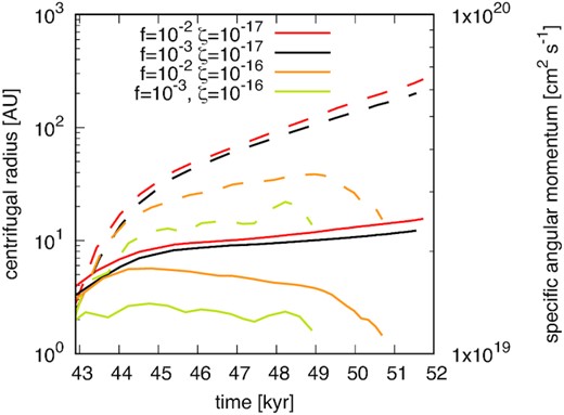
Time evolution of the centrifugal radius (solid lines; left axis) and specific angular momentum (dashed lines; right axis). The red, black, orange, and yellow lines show the results of model_MRN_f1e2_zeta1e17, model_MRN_f1e3_zeta1e17, model_MRN_f1e2_zeta1e16, model_MRN_f1e3_zeta1e16, respectively.
The dashed line in Fig. 4 shows the time evolution of the specific angular momentum of the disc. The specific angular momentum increases after the disc forms in both the low and high cosmic ray ionization rate models. In low models (red and black lines), it continues to increase with time, but in high models (orange and yellow lines), it declines after about 5000 years. Because gas is well-coupled with magnetic fields in the high cosmic ray ionization rate models, the magnetic braking is stronger in these models than in the lower models. As a result, the gas loses its angular momentum, and the disc is disappeared in the high cosmic ray ionization rate models.
3.4 Time evolution of the mass of protostar and disc
In this section, we investigate the time evolution of Mdisc, Mstar, and Mdisc + Mstar. Disc mass is defined as the enclosed mass within ρ > ρdisc = 10−14 g cm−3.
Fig. 5 shows the time evolution of disc mass Mdisc (solid), and protostar mass Mstar (dashed). At t = 4.3 × 10⁴ yr, the disc mass (solid) is comparable (|$M_{\rm {disc}}\sim 0.2\, {\rm M}_{\odot }$|) in model_MRN_f1e2_zeta1e17, model_MRN_f1e3_zeta1e17, and model_MRN_f1e2_zeta1e16. While model_MRN_f1e3_zeta1e16 has a smaller disc mass. With time, Mdisc increases in low cosmic ray ionization models (red and black lines), but in high cosmic ray ionization models (orange and yellow lines), Mdisc rapidly decreases at t ∼ 4.7 × 10⁴ and 4.9 × 10⁴ yr, respectively. This property is the same as disc radius and angular momentum (see Fig. 4).
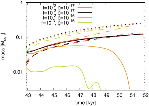
Time evolution of the mass of disc Mdisc (solid lines), protostar Mstar (dashed lines), and Mdisc + Mstar (dotted lines). The red, black, orange, and yellow lines show the results of model_MRN_f1e2_zeta1e17, model_MRN_f1e3_zeta1e17, model_MRN_f1e2_zeta1e16, and model_MRN_f1e3_zeta1e16, respectively.
On the other hand, the total masses of the protostars and discs (dotted) are almost the same for all models. This indicates that the mass carried away by the outflow is sufficiently small and that the disappearance of the disc is due to mass accretion onto the central protostar.
3.5 Time evolution of outflow
In this section, we investigate the properties of outflow. An outflow is defined as a region that satisfies |$v_r = (\mathbf {v}\cdot \mathbf {r})/|\mathbf {r}| > 2c_{\rm {s,ios}}$| and ρ < 10−14 g cm−3, where |$c_{\rm {s,ios}}=0.19\,{\rm km\,s}^{-1}$| is sound velocity at |$T=10\,{\rm K}$|. This definition matches that in Tsukamoto et al. (2020). Outflows are formed in all models.
Fig. 6 shows the time evolution of the outflow size. The outflow size is defined as the distance at which the particles in the outflow are farthest from the central protostar. In our simulations, a strong outflow with velocity |$v > 1\,{\rm km\,s}^{-1}$| forms a few thousand years after protostar formation. The size of the outflow increases monotonically. In t ∼ 9.0 × 10³ yr after outflow formation with low cosmic ray ionization (red and black), the outflow size reaches ∼2000 au with both low and high dust fraction. The average velocity of the outflow is thus |$1.1\,{\rm km\,s}^{-1}$|. With high cosmic ray ionization, the outflow size reaches ∼3000 au at t ∼ 8.0 × 10³ yr (model_MRN_f1e2_zeta1e16, orange line) and t ∼ 6.0 × 10³ yr (model_MRN_f1e3_zeta1e16, yellow line) from the protostar formation. Thus, the average velocity of the outflow head is found to be |${\sim}1.8\,{\rm km\,s}^{-1}$| for model_MRN_f1e2_zeta1e16 (orange), |${\sim}2.4\,{\rm km\,s}^{-1}$| for model_MRN_f1e3_zeta1e16 (yellow). This result indicates that high cosmic ray ionization models have about twice the velocity of low cosmic ray ionization models.
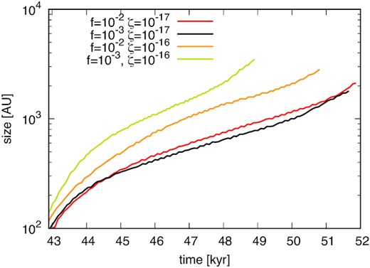
Time evolution of the size of outflow. The red, black, orange, and yellow lines show the results of model_MRN_f1e2_zeta1e17, model_MRN_f1e3_zeta1e17, model_MRN_f1e2_zeta1e16, and model_MRN_f1e3_zeta1e16, respectively.
Fig.7 shows the time evolution of the outflow mass. In all models, the outflow mass is monotonically increasing. Outflow mass is inversely correlated with disc mass, suggesting that outflow activity is related to disc growth. Models with a high cosmic ray ionization rate have larger masses than those with a low ionization rate. Regarding the dust fraction, the low dust fraction model (yellow) has a more active outflow than the high dust fraction model (orange) with high cosmic ray ionization. Thus, Fig. 7 suggests also that the dust fraction affects the evolution of outflow in a high cosmic ray ionization environment.
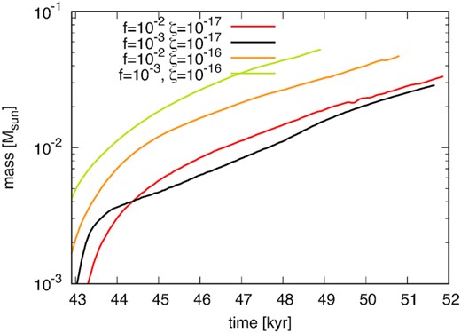
Time evolution of the mass of outflow. The red, black, orange, and yellow lines show the results of model_MRN_f1e2_zeta1e17, model_MRN_f1e3_zeta1e17, model_MRN_f1e2_zeta1e16, and model_MRN_f1e3_zeta1e16, respectively.
Fig.8 shows the time evolution of the outflow specific angular momentum. The dust fraction has little effect on the specific angular momentum of the outflow. If we compare the high and low cosmic ray ionization, the difference among the models is about a factor of two at the end of the simulation. This means that the outflow will more efficiently remove the angular momentum from the central region in high cosmic ray ionization models. Therefore, in models with a high cosmic ray ionization rate, the disc disappears at the end of the simulation. This suggests that the high cosmic ray ionization environments have a more active outflow and that the angular momentum is removed from the disc.
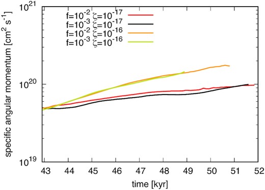
Time evolution of the specific angular momentum of outflow. The red, black, orange, and yellow lines show the results of model_MRN_f1e2_zeta1e17, model_MRN_f1e3_zeta1e17, model_MRN_f1e2_zeta1e16, and model_MRN_f1e3_zeta1e16, respectively.
4 DISCUSSION
4.1 Impact on disc formation
In all models considered in this paper, the circumstellar disc is formed at t ∼ 4.3 × 10⁴ yr. At the time of the formation, the centrifugal radius and mass of the discs were 2–4 au and |$0.01\!-\!0.02 \,{\rm M}_{\odot }$|, respectively. It is also shown that discs can grow at low cosmic ray ionization rates (|$\zeta _{\rm {CR}}=10^{-17}\rm {s^{-1}}$|), but disappear at high cosmic ray ionization rates (|$\zeta _{\rm {CR}}=10^{-16}\,{\rm s}^{-1}$|). Figs 2 and 4 show a result that is consistent with the results of Kuffmeier et al. (2020) in which the formation of the disc strongly depends on the cosmic ray ionization rate.
Dust fraction, on the other hand, refers to the amount of dust grains in the cloud. Dust grains are sinks for electrically charged particles. Therefore, as the dust fraction decreases, the resistivity in the central region decreases (conductivity increases). Therefore, it is expected that the removal of angular momentum by magnetic braking would be more efficient, suppressing the formation and evolution of discs in low dust fraction models (|$Z=0.1\,Z_{\odot }$|). However, our results did not show as pronounced a difference as the difference in cosmic ray ionization. Thus, in the parameter range we considered, disc formation is more strongly affected by cosmic ray ionization than by dust fraction.
4.2 Activity of outflow
Outflow is one of the mechanisms that remove angular momentum from the central region. In this simulation, outflows form in all models, even with different cosmic ray ionization rates and dust fractions. We found that the nature of the outflow does differ depending on the cosmic ray ionization rate and dust fraction. For example, the timing of outflow formation is earlier in models with a high cosmic ray ionization rate than in models with a low rate. In the case of a high cosmic ray ionization rate, the mass and angular momentum of the outflow are larger for the low dust fraction model (model_MRN_f1e3_zeta1e16) than for the high dust fraction model (model_MRN_f1e2_zeta1e16). On the other hand, within the low cosmic ray ionization models, there is little difference depending on the dust fraction.
Fig.9 plots the momentum F per unit time injected into the outflow versus the luminosity of the central source L (Wu et al. 2004, which can be compared with fig. 7).
Here,
where Δt is the time after the launching of the outflow and f is the ratio that the gravitational potential converts to radiational energy, and f = 0.25. In high cosmic ray ionization models (orange and yellow lines), F is larger than in low models (red and black lines), and the luminosity rapidly increases at the end of simulations. This rapidly increasing luminosity is due to the disc gas rapidly falling on the central object. While low cosmic ray ionization models do not have rapidly increasing luminosity at the end of simulations, they do have rapidly decreasing luminosity. However, in low cosmic ray ionization models, outflow momentum rapidly increases at the end of the simulation.
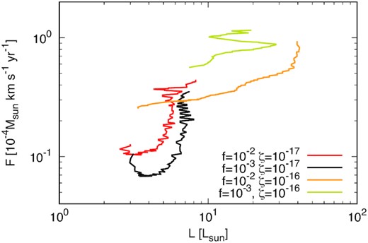
Outflow force F versus luminosity. The luminosity is calculated with equation (3) in Stamatellos, Whitworth & Hubber (2012). The red, black, orange, and yellow lines show the results of model_MRN_f1e2_zeta1e17, model_MRN_f1e3_zeta1e17, model_MRN_f1e2_zeta1e16, and model_MRN_f1e3_zeta1e16, respectively. The arrows show the direction of time evolution.
From Fig. 9, we suggest that outflow momentum differs depending on the environment, such as cosmic ray ionization rate and dust fraction. For instance, in fig. 7 of Wu et al. (2004), the plots are scattered not only along the horizontal axis (luminosity) but also along the vertical axis (outflow momentum per unit time). Horizontal scattering is thought to be due to the time evolution of the objects. However, it is not clear whether vertical scattering is due to the evolution of objects or not. In Fig. 9, there is a clear difference among the models. For instance, models with a high cosmic ray ionization rate have greater outflow momentum than ones with a low cosmic ray ionization rate. Thus, the environment of a star-forming region may affect the outflow momentum through the difference in ionization.
5 SUMMARY
In this paper, we study the formation and early evolution of young stellar objects (YSOs) using three-dimensional non-ideal MHD simulations to investigate the effect of cosmic ray ionization rate and dust fraction (or amount of dust grains) on circumstellar disc formation. Our results are summarized as follows:
Circumstellar discs are formed in all simulations at t ∼ 4.3 × 10⁴ yr. Discs eventually grow up r ∼ 10 au in low cosmic ray ionization models (model_MRN_f1e3_zeta1e17 and model_MRN_f1e2_zeta1e17), however, they disappear in high cosmic ray ionization models (model_MRN_f1e3_zeta1e16 and model_MRN_f1e2_zeta1e16) at the end of simulations. While the impact on disc formation and evolution of the dust fraction is smaller than the cosmic ray ionization rate.
All simulations were outflow driven. In high cosmic ray ionization and low dust fraction models, the outflow has a greater angular momentum and outflow force. Thus, the cosmic ray ionization rate and dust fraction can influence outflow formation and evolution.
ACKNOWLEDGEMENTS
We thank the anonymous referee for her/his insightful comments. A Cray XC50 at the Center for Computational Astrophysics at the National Astronomical Observatory of Japan was used to calculate the simulation. This work is supported by JSPS KAKENHI grant numbers JP18H05437 and JP21J23102.
DATA AVAILABILITY
The simulation data will be shared on reasonable request with the corresponding author.
References
A
