


ABSTRACT
Time-domain astronomy is entering a new era as wide-field surveys with higher cadences allow for more discoveries than ever before. The field has seen an increased use of machine learning and deep learning for automated classification of transients into established taxonomies. Training such classifiers requires a large enough and representative training set, which is not guaranteed for new future surveys such as the Vera Rubin Observatory, especially at the beginning of operations. We present the use of Gaussian processes to create a uniform representation of supernova light curves from multiple surveys, obtained through the Open Supernova Catalog for supervised classification with convolutional neural networks. We also investigate the use of transfer learning to classify light curves from the Photometric LSST Astronomical Time Series Classification Challenge (PLAsTiCC) data set. Using convolutional neural networks to classify the Gaussian process generated representation of supernova light curves from multiple surveys, we achieve an Area Under the Receiver Operating Characteristic curve (AUC) score of 0.859 for classification into Types Ia, Ibc, and II. We find that transfer learning improves the classification accuracy for the most under-represented classes by up to 18 per cent when classifying PLAsTiCC light curves, and is able to achieve an AUC score of 0.946 ± 0.001 when including photometric redshifts for classification into six classes (Ia, Iax, Ia-91bg, Ibc, II, and SLSN-I). We also investigate the usefulness of transfer learning when there is a limited labelled training set to see how this approach can be used for training classifiers in future surveys at the beginning of operations.
1 INTRODUCTION
The emergence of synoptic all-sky surveys with increased coverage of the night sky (both in area and in time) has allowed astronomers to discover more objects more quickly (e.g. Pan-STARRS, Kaiser et al. 2010; Asteroid Terrestrial-impact Last Alert System, Tonry et al. 2018; All Sky Automated Survey for SuperNovae, Shappee et al. 2014; the Gravitational-wave Optical Transient Observer (GOTO), Steeghs et al. 2021; Zwicky Transient Facility, Bellm et al. 2019). The rate of discovery and data collection of current surveys and that of expected future surveys such as the Legacy Survey of Space and Time (LSST; Ivezić et al. 2019) on the Vera Rubin Observatory have prompted work on machine learning and deep learning approaches to automate the identification and classification of new transients. The motivation for photometric classification of supernovae arises from the fact that not all discovered supernovae will be subject to spectroscopic follow-up for spectral classification. The ability to classify supernovae based on just light curves will benefit the studies of cosmology with Type Ia supernovae (Riess et al. 1998; Perlmutter et al. 1999; Betoule et al. 2014) and accumulating a large sample of core-collapse supernovae allows for population studies to understand their diversity (e.g. Modjaz, Gutiérrez & Arcavi 2019). In the past decade, a lot of work has been done on supernova light-curve classification using photometric observations with machine learning and deep learning. At present, most of these studies focus on classifying supernovae from a single survey with either real or simulated data.
Lochner et al. (2016) and Charnock & Moss (2017) used simulated supernova light curves from the Supernova Photometric Classification Challenge (SPCC; Kessler et al. 2010) to classify supernovae into three classes (Ia, Ib/c, and II). Muthukrishna et al. (2019) used a recurrent neural network to classify simulated Zwicky Transient Facility (ZTF) light curves of various explosive transients, including supernovae. Pasquet et al. (2019) used a convolutional neural network to classify supernova light curves from multiple data sets (SPCC, simulated LSST, and Sloan Digital Sky Survey), capable of handling irregular sampling of light curves and a non-representative training set. Möller & de Boissière (2020) developed a deep neural network approach to classify a set of simulated supernova light curves similar to the SPCC data set, capable of classification on incomplete light curves. Dauphin et al. (2020), Hosseinzadeh et al. (2020), and Villar et al. (2019) created classifiers trained on light curves of spectroscopically confirmed Pan-STARRS1 supernovae. Takahashi et al. (2020) used a neural network to classify supernova light curves from the Hyper Suprime-Cam transient survey. In Burhanudin et al. (2021), we presented a recurrent neural network for classifying light curves from the GOTO survey, capable of handling an imbalanced training data set. In all the examples listed above, the overall classification performance is good for a number of classification tasks (binary Ia/non-Ia or a multiclass problem into the different supernova subtypes), achieving accuracies of |$\gtrsim 85{{\ \rm per\ cent}}$|.
The aforementioned studies all focus on classifying supernova light curves that have been obtained from a single survey or simulated to resemble the light curves of a particular survey. Pruzhinskaya et al. (2019) used supernova light curves from multiple surveys, obtained from the Open Supernova Catalog (Guillochon et al. 2017) to develop an anomaly detection algorithm, capable of identifying rare supernova classes and non-supernova objects within the data set. The challenge in working with light curves from different surveys is dealing with differences in how the photometry is calibrated, and the different filters used when making observations. By having a classifier that is agnostic to differences across different surveys, it allows the use of more available survey data so that the training of classifiers is not limited to the size of a sample obtained from just a single survey. We expand on the literature by applying a deep learning approach to classification on a heterogeneous data set of supernova light curves, combined from multiple surveys. Using light curves from multiple surveys that use different filters also allows access to a wider wavelength coverage in broad-band photometric observations.
One approach to working with a heterogeneous data set is to find a way to standardize the data, so that they are represented in a more uniform manner. Boone (2019) used a Gaussian process to model simulated LSST light curves from the Photometric LSST Astronomical Time Series Classification Challenge data set (PLAsTiCC; The PLAsTiCC Team 2018), by interpolating in both time and wavelength. Gaussian processes have also been used to generate a 2D representation of supernova light curves (Qu & Sako 2021; Qu et al. 2021), which are then used as inputs to a convolutional neural network for classification. By using a Gaussian process to interpolate light curves in time and wavelength, it is possible to create a uniform representation of light curves that consist of observations made across different filters.
A challenge in creating classifiers for new surveys is the lack of a labelled training set with which to train a model. Many machine learning and deep learning classification methods assume that the training and test data come from the same distribution and share a common feature space. When the distribution changes, the models need to be retrained with a new labelled training set. In most cases, creating a new labelled training set to account for the change in distribution can be extremely difficult. Transfer learning (Pan & Yang 2010) is an approach that uses the knowledge gained in performing a task (e.g. classification) in one domain (e.g. data from one particular survey) to perform another task in a different domain (e.g. classification using data from a different survey).
In this paper, we use Gaussian processes to create a uniform representation of supernova light curves from multiple surveys obtained through the Open Supernova Catalog, and use convolutional neural networks to classify the supernovae into different types. We also investigate the use of transfer learning to classify light curves from the PLAsTiCC data set, using domain knowledge derived from the task of classifying Open Supernova Catalog light curves. In Section 2, we introduce data from the Open Supernova Catalog, and in Section 3 we present a 2D Gaussian process to generate a 2D representation of supernova light curves. Section 4 introduces the convolutional neural network used for classification. We present the results of classifying Open Supernova Catalog data in Section 5. We introduce transfer learning and the PLAsTiCC data in Section 6, and results on classifying PLAsTiCC data in Section 7. We provide a discussion of the work presented in this paper and conclude in Section 8.
2 OPEN SUPERNOVA CATALOG DATA
Supernova light curves and metadata (such as the supernova classification obtained via spectroscopy or through expert human inspection, any available spectroscopic data, and the RA and Dec.) were retrieved from the Open Supernova Catalog website.1 The downloaded data consisted of supernovae listed on the Open Supernova Catalog discovered up to the end of 2019, totalling 80 914 objects. All objects that were labelled as ‘Candidate’ or other non-supernova classes were discarded. Only objects that had been labelled as types Ia, Ibc, or II (including all sub-classifications within those types) were kept. For supernovae that had multiple labels, we only consider those that contained multiple labels of the same type (e.g. Ib/c or Ib) and discarded those with conflicting labels.
2.1 Standardizing magnitudes and filters
The light curves in the Open Supernova Catalog data set consist of observations that have been made with a variety of instruments across a number of different telescopes. In Fig. 1, we plot the full width at half-maximum (FWHM) against the effective wavelength for the filters used in the data set. The values for the effective wavelength and FWHM for the filters in Fig. 1 were obtained from the Spanish Virtual Observatory (SVO) Filter Profile Service (Rodrigo & Solano 2020).2
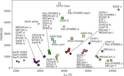
A plot of FWHM against the effective wavelength λeff of the filters available in the Open Supernova Catalog data set. Both λeff and FWHM are given in angstroms.
The data set also contains photometry generated using models or simulations and we discard these and only keep real photometric observations. Where available we use the system column in the photometry data to identify which magnitude system the data is calibrated to, otherwise the instrument column is used to identify which instrument was used to make the observation. The next step is then to convert all the magnitudes so that they are in the same magnitude system. The majority of magnitudes in the data set are given in the AB magnitude system, so we convert the rest of the magnitudes into AB magnitudes. Magnitudes given in systems other than AB were converted using Tables A1, A2, and A3 listed in the appendix. After converting all magnitudes into the AB system, the magnitudes were then converted into flux (in units of erg s−1 Hz−1 cm−2) using:
where fν is the monochromatic flux and mAB is the AB magnitude.
2.2 Light-curve trimming
Some light curves in the data set span periods of up to multiple years, including seasonal gaps and periods where the only photometry available is actually of the host galaxy without the supernova. To shorten these longer light curves, so that we just consider the supernova, the steps listed below are taken:
Long light curves (longer than 300 d of observations) were split into shorter light-curve chunks if there is a gap in observations longer than 60 d.
Compare the standard deviation in magnitudes of each light-curve chunk σchunk to the standard deviation of the whole light curve σlc.
If σchunk < σlc, then that portion of the light curve is discarded.
Fig. 2 shows some example trimmed light curves. We find that this method is good at isolating the rise, peak, and decline of supernovae in the Open Supernova Catalog data set.
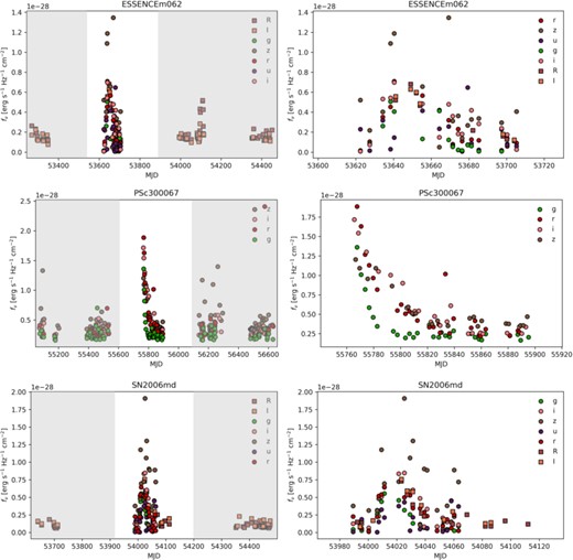
Light curves from the Open Supernova Catalog, before (left) and after trimming (right). The shaded regions on the left indicate parts of the light curves that were discarded.
2.3 Selection cuts
To create the final data set, the following selection cuts were made:
Total number of observations in the light curve is ≥6.
At least two or more filters used.
The average number of observations per filter is ≥2.
The length of observations spans at least 20 or more days.
These cuts were made to ensure that the light curves had good coverage across multiple wavelengths and in time so that there was enough information in each light curve to allow a model to learn to differentiate between the different classes. Good quality light curves are also required to ensure the light curve has enough data points to provide a good fit with Gaussian processes.
After the cuts, the number of remaining objects in our sample is 6330 of the total. The data set is split into 60 per cent for training (3796 objects), 15 per cent for validation (951), and 25 per cent for testing (1583). The data is split into three classes for the classification task: Ia, Ibc, and II. The proportion of each class in the training, validation and test set is the same. This is done to ensure that there are a sufficient number of samples from each class in the validation and test set to evaluate classification performance across all classes, including those with fewer samples.
Table 1 summarizes how the data set is partitioned. Type Ia and II supernovae make up the majority of objects in the data set, with only a small proportion of type Ibc supernovae in the data. This data set presents a class imbalance problem, where one class contains fewer examples compared to other classes. Learning from an imbalanced data set can be difficult, since conventional algorithms assume an even distribution of classes within the data set. Classifiers will tend to misclassify examples from the minority class, and will be optimized to perform well on classifying examples from the majority class (see Burhanudin et al. 2021).
A breakdown of how the final Open Supernova Catalog data set (after light-curve trimming and selection cuts) is divided for training, validation, and testing, along with the class distribution of the three supernova classes.
| Type | Training | Validation | Test | All data |
|---|---|---|---|---|
| Ia | 2145 (56.5 per cent) | 542 (57.0 per cent) | 883 (55.8 per cent) | 3570 (56.4 per cent) |
| II | 1563 (41.2 per cent) | 385 (40.5 per cent) | 657 (41.5 per cent) | 2605 (41.2 per cent) |
| Ibc | 88 (2.3 per cent) | 24 (2.5 per cent) | 43 (2.7 per cent) | 155 (2.4 per cent) |
| Total: | 3796 | 951 | 1583 | 6330 |
3 GAUSSIAN PROCESSES FOR INTERPOLATION IN TIME AND WAVELENGTH
3.1 Gaussian processes
A Gaussian process can be thought of as a non-parametric modelling method based on the multivariate Gaussian. Gaussian process regression attempts to find a function f(x) given a number of observed points y(x) that determines the value y(x′) for unobserved independent variables x′ (over a finite interval of x′ values) by drawing from a distribution of functions. The distribution of functions is determined by selecting a covariance function (also referred to as kernels), which specifies the covariance between pairs of random variables. Covariance functions have adjustable hyperparameters, which determine the form of the Gaussian process prediction for f(x). For a detailed discussion on Gaussian processes see Rasmussen & Williams (2005).
3.2 2D Gaussian process regression
In order to create a uniform representation of light curves in different filters, we follow the approach used in Qu et al. (2021) and Boone (2019), and use 2D Gaussian process regression to interpolate the light curves in wavelength and time. We model the light curves to create a 2D image (referred to as a ‘flux heatmap’ in Qu et al. 2021 and Qu & Sako 2021) where the flux is given as a function of time t and wavelength λ.
We label each flux measurement in all light curves in the data set with the effective wavelength λeff of the filter in which it was observed. The values for λeff for each filter are listed in Table 2, and are obtained from the SVO Filter Profile Service (Rodrigo & Solano 2020) and Blanton & Roweis (2007). Observations covering wavelengths from the Swift UVW2 filter (with λeff = 2085.73 Å) up to the Johnson–Cousins J filter (with λeff = 12 355.0 Å) were used. These filters were used as the vast majority of observations in the data set were made using filters within this wavelength range. All flux values of each light curve are associated with a time measurement t (time of observations) and a wavelength value λeff, the effective wavelength of the filter used to make the observation. We scaled the time so that the time of the first observations is t = 0.
The effective wavelengths λeff of the filters used to create flux heatmaps from the light curves in our sample dervied from the Open Supernova Catalog.
| Filter | λeff (Å) |
|---|---|
| UVW2 | 2085.73 |
| UVW1 | 2684.14 |
| UVM2 | 2245.78 |
| U | 3751.0 |
| B | 4344.0 |
| V | 5456.0 |
| R | 6442.0 |
| I | 7994.0 |
| J | 12355.0 |
| u | 3546.0 |
| g | 4670.0 |
| r | 6156.0 |
| i | 7472.0 |
| z | 8917.0 |
| y | 10305.0 |
| Filter | λeff (Å) |
|---|---|
| UVW2 | 2085.73 |
| UVW1 | 2684.14 |
| UVM2 | 2245.78 |
| U | 3751.0 |
| B | 4344.0 |
| V | 5456.0 |
| R | 6442.0 |
| I | 7994.0 |
| J | 12355.0 |
| u | 3546.0 |
| g | 4670.0 |
| r | 6156.0 |
| i | 7472.0 |
| z | 8917.0 |
| y | 10305.0 |
As in Qu et al. (2021) and Boone (2019), we use the Matérn 3/2 covariance function in our 2D Gaussian process, with a fixed characteristic length-scale in wavelength of 2567.32 Å, which is obtained by dividing the wavelength range covered by all the filters in Table 2 by 4. We note that this value is arbitrary, and that other values of fixed characteristic length scale could be used. From Fig. 1, one could use the FWHM of the filters to inform the choice of length-scale. Boone (2019) find that their analysis on using Gaussian processes to model light curves is not sensitive to the choice of the length-scale in wavelength, so we do not investigate this choice further. We leave the time length-scale as a trainable parameter. The Matérn 3/2 kernel has the form:
where σ2 is the variance parameter, which is left as a trainable parameter, and r is the Euclidean distance between two input points x1 and x2, scaled by a length-scale parameter l (which we leave as a fixed constant):
The kernel used for the 2D Gaussian process regression to model the light curves in wavelength and time is:
where rλ is the Euclidean distance between the wavelength input points, scaled by the fixed wavelength length-scale parameter, and rt is the Euclidean distance between the time input points, scaled by the time length-scale parameter.
The 2D Gaussian process is trained on each light curve in the data set, and then used to predict flux measurements on a time-wavelength grid. The wavelength dimension in the grid runs from 2085.73 to 12355.0 Å divided into 25 bins resulting in a wavelength interval of 410.77 Å, and the time dimension runs from 10 d before and 110 d after the first observation with an interval of 1 d. In Section 6.5, we use this approach to generate flux heatmaps for 397 990 PLAsTiCC supernova light curves, so the choice of dimensions is a practical one. The resulting flux heatmap image has dimensions of 120 × 25 pixels, where each pixel represents a flux measurement. Fig. 3 shows example flux heatmaps. The flux heatmaps are used as input for a convolutional neural network for classification. We use the GPFlowpython package (Matthews et al. 2017) to perform Gaussian process regression. The time taken to generate a flux heatmap from a light curve with a Gaussian process on a 4-core CPU is approximately 3 s.
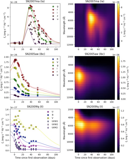
Examples of light curves (left) of SN2007ma (type Ia), SN2005aw (type Ibc), and SN2009lq (type II) and the corresponding flux heatmaps (right) generated using a 2D Gaussian process. The light curves are plotted as flux fν converted from AB magnitudes in each filter against time. Also plotted with the light curves are the Gaussian process fits in each band. The heatmaps show flux (brighter pixels indicating higher flux values) as a function of time (in days) and wavelength (in Å).
3.3 Using 2D Gaussian processes to infer spectra from light curves
The 2D Gaussian process regression can be used as a method to infer supernova spectra from their light curves. We select iPTF13bvn from the Open Supernova Catalog data set as an example. This is a type Ib supernova that has good photometric coverage in time and across multiple filters. Fig. 4 shows the light curve and the corresponding flux heatmap generated with a 2D Gaussian process.

The light curve of the type Ib supernova iPTF13bvn (left) and its flux heatmap generated from the light curve (right).
We examine three spectra for iPTF13bvn, made available through the Open Supernova Catalog (Guillochon et al. 2017; Shivvers et al. 2019). To obtain the ‘simulated’ spectra from the flux heatmap, we take a single column at the time the spectra were taken, giving a vector that measures flux as a function of wavelength. The time of observation of the spectra is scaled to the time of first observation in the light curve, so it is given as the number of days since the first light curve observation. The real spectra for iPTF13bvn are taken at 20.6, 23.7, and 47.5 d after the first light-curve observation, so the corresponding simulated spectra are obtained by taking columns from the flux heatmap at 20, 24, and 48 d after the first light-curve observation. Fig. 5 compares the real spectra of iPTF13bvn to the simulated spectra obtained from the flux heatmap.
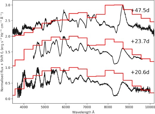
The spectra of iPTF13bvn are shown in black, and the spectra obtained from the flux heatmap are shown in red. The time of the spectra is given as days from the time of the first observation of the light curve. The spectra have been normalized (using the maximum value for each individual spectra) and shifted for clarity.
From Fig. 5, it can be seen that the spectra generated from the flux heatmap correlate quite well with the real spectra of iPTF13bvn. In all three spectra, the heatmap generated spectra appear to trace the continuum shape. For the spectra obtained at 47.5 d, the heatmap generated spectrum correlates with the Ca II IR triplet emission feature at ∼8700 Å. Although there is a correlation, there is a poor match between the real spectrum and the heatmap generated spectrum which could be due to the width of the red filters (see Fig. 1). Here, we have shown one example where the 2D Gaussian process to create a flux heatmap can be used to generate low resolution spectra, provided there is good photometric coverage across multiple filters. In this example, photometric data for iPTF13bvn was obtained from three different sources across 12 different filters.
4 CONVOLUTIONAL NEURAL NETWORKS
4.1 Model architecture
Convolutional neural networks (CNNs; Lecun 1989) are a class of neural networks that can process data with a grid-like structure (e.g. a 2D grid of pixels in an image, or a sequence of measurements in time-series data where there may be one or more measurements at each time-step). CNNs use convolution filters to identify spatial features in the data (such as corners or edges in an image). The output of a convolution applied to the input data is referred to as a ‘feature map’
We use a CNN to classify the flux heatmaps created from the Open Supernova Cataolog light curves (Section 3.2) into three different classes: supernovae of types Ia, Ibc, and II. We build the CNN using the TensorFlow 2.0 package for python (Abadi et al. 2016)3 with Keras (Chollet et al. 2015) for implementation of network layers.
The input to the CNN is a 2D flux heatmap image of a supernova light curve, with dimensions 120 × 25 pixels where each pixel represents a flux density value. All flux heatmaps are normalised by dividing by the highest flux density value, so that the pixels in every heatmap have values between 0 and 1. We use a CNN with three convolutional blocks, followed by two fully connected layers before the final output layer. Each convolutional block consists of a convolution layer, a batch normalization layer, and a 2 × 2 max pooling layer. Fig. 6 illustrates the model architecture used. For the convolutional and dense layers, the rectified linear unit (ReLU) activation function is used, and in the final output layer the softmax activation function is used to produce a list of probabilities that sum to unity. The probabilities returned by the model are scores that describe the level of ‘belongingness’ to a class.
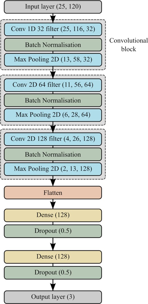
A diagram of the convolutional neural network used in this paper. The grey dashed box indicates the layers that make up a convolutional block. The dimensions of the output tensors in the layers in the convolutional blocks (Conv 1D, Conv 2D, and Max Pooling 2D), number of neurons in the dense layers (Dense), and the dropout fractions (Dropout) are shown in parentheses.
In the first convolutional block we apply a 1D convolution (also called a temporal convolution) in the time dimension instead of a standard 2D convolution. This is done since the flux heatmap is generated from a light curve which measures the brightness of a supernova over time, so we attempt to extract temporal features in the first convolutional block and see if the CNN considers the evolution of flux as a function of wavelength in time. An alternative approach is to use the conventional 2D convolution for feature extraction as is conventionally done for image classification.
The output of each convolutional block has dimensions (nrows, ncolumns, and nfilters), where nfilters is a convolutional layer parameter and refers to the number of convolution filters used to generate feature maps. In the second and third convolutional blocks, a 2D convolution is applied to the output of the preceding convolutional block. Table 3 lists the series of convolutions and max pooling applied in the convolutional blocks, with the corresponding layer parameters and output dimensions at each stage.
The layer parameters and output dimension for each layer in the convolutional blocks. For the convolutional layers, the kernel size is the shape of the convolutional window and filters sets the number of convolutional filters that are learnt during training. For the max pooling layers, the pool size sets the shape of the window over which to take the maximum. The number of strides is one for the convolutional layers and two for the max pooling layers. The flattening layer takes the multidimensional output of the convolutions and shapes it into a single dimensional output.
| Layer | Kernel/Pool size | Filters | Output dimension |
|---|---|---|---|
| Conv 1D | (5) | 32 | (25, 116, 32) |
| BatchNorm | – | – | (25, 116, 32) |
| MaxPool 2D | (2,2) | – | (13, 58, 32) |
| Conv 2D | (3,3) | 64 | (11, 56, 64) |
| BatchNorm | – | – | (11, 56, 64) |
| MaxPool 2D | (2,2) | – | (6, 28, 64) |
| Conv 2D | (3,3) | 128 | (4, 26, 128) |
| BatchNorm | – | – | (4, 26, 128) |
| MaxPool 2D | (2,2) | – | (2, 13, 128) |
| Flatten | – | – | 3328 |
The output of the last convolutional block is then flattened into a 1D vector and then passed on to two fully connected layers, each with dropout applied with the dropout fraction set to 0.5. We apply a L2 regularization in the second fully connected layer with a regularization parameter of 0.01, which is the default TensorFlow value. The final output layer is a fully connected layer with the same number of neurons as the number of classes, which is three. In total, the CNN model has 536,003 trainable parameters.
4.2 Model training
The CNN model is trained on the flux heatmaps generated from the Open Supernova Catalog light curves with a learning rate of 1 × 10⁻⁵ for 1500 epochs with the Adam optimizer (Kingma & Ba 2014), using a batch size of 128. Fig. 7 shows how the training and validation loss evolve with training. Within 1500 epochs of training, both the training and validation loss begin to converge (i.e. stops improving). We use a cross-entropy loss (CE) function, weighted to take into account the class imbalance present in the data. Given a multi-class problem with N classes, the CE loss for an example i is:
where pij is the probability of example i belonging to class j, αj is the class weight for class j, and δij is the Kronecker delta function. The loss for the entire data set is given by summing the loss of all examples. The class weight αj for class j is
where n is the total number of classes, N is the total number of samples in the data set, and Nj is the number of samples in class j. The class weights are obtained using samples in the training set.
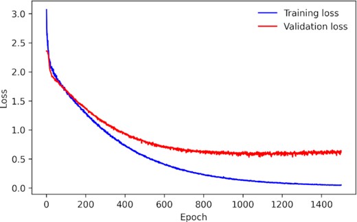
The training and validation loss for the CNN model trained on the Open Supernova Catalog data.
The model is trained on an NVIDIA Quadro P2200 graphics processing unit with 1280 cores and 5 GB of memory, which takes 4 s per epoch for a total time of ∼100 min to train the model.
5 RESULTS ON CLASSIFYING OPEN SUPERNOVA CATALOG DATA
Once the model has been trained, it is then used to make predictions on the test set. The test set consists of data that is kept apart from the training and validation sets, and used to evaluate how well the model is able to generalize on unseen data. On the test set, the model achieves an Area Under the Receiver Operating Characteristic curve (AUC) score of 0.859, and an F1 score of 0.708. Fig. 8 shows the confusion matrix for the model evaluated with the test set.
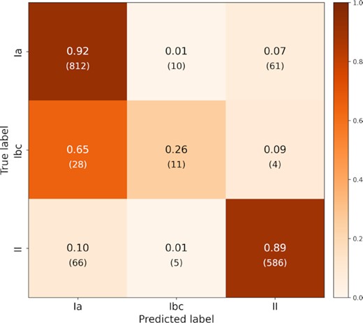
Confusion matrix for the test set of flux heatmaps generated from the Open Supernova Catalog light curves. The y-axis shows the true class label, and the x-axis shows the class label predicted by the model. Entries along the diagonal represent where the predicted label matches the true label, and the off-diagonal entries show where misclassifications occur. Reading along the rows, the fractional values show how samples from a class have been classified, with the absolute numbers below in parentheses.
From the confusion matrix, the model shows good classification of Type Ia and II supernovae with 92 per cent (812) and 89 per cent (586) accuracy for each class, respectively. The performance for Type Ibc supernovae is poor, with the model only achieving 26 per cent (11) accuracy for that class and misclassifying 65 per cent (28) of Type Ibc supernovae as Type Ia. This may be due to the small number of samples of Type Ibc supernovae in the data set. The majority of Type Ibc supernovae are misclassified as Type Ia, and it is known that it can be challenging to differentiate between Type Ia and Type Ibc with only photometry (Lochner et al. 2016). The misclassifications between Type Ia and Type II are quite low, with |$\lesssim ~10{{\ \rm per\ cent}}$| (61 for Type Ia and 66 for Type II) of each being misclassified as the other.
Dobryakov et al. (2021) used a machine learning approach for the binary classification problem of Type Ia versus non-Ia supernova classification using light curves from the Open Supernova Catalog. They find that they achieve a best AUC score of 0.876 and a best F1 score of 0.917. However, they only consider classifying light curves using r-band observations and a data set of 1184 Type Ia and 344 non-Ia supernovae.
6 TRANSFER LEARNING ON PLASTICC SUPERNOVA LIGHT CURVES
6.1 Overview
In the case of a classification task where there is a lack of labelled training data, the ability to transfer classification knowledge from one domain to a new one is useful. In astronomy, new surveys can experience the problem of a small or complete lack of a labelled training set since it can take time to accumulate enough sources and also label them (e.g. using spectroscopy or visual inspection of the photometry). In the following sections, we present the application of transfer learning to classify supernova light curves from the PLAsTiCC data set (The PLAsTiCC Team 2018) by using classification knowledge derived from the Open Supernova Catalog light curves presented in the previous sections.
Transfer learning is defined as improving the learning of a target predictive function (e.g classification, mapping inputs to a class) in a target domain |$\mathcal {D}_T$| using knowledge from a source domain |$\mathcal {D}_S$| and source task |$\mathcal { T}_S$| (Pan & Yang 2010). In this case, the target domain is the PLAsTiCC data set, the source domain is the Open Supernova Catalog data set, the source task is classifying Open Supernova Catalog light curves into one of three classes (Ia, Ibc, and II), and the target predictive function is classifying light curves from the PLAsTiCC data set.
6.2 The PLAsTiCC data set
The PLAsTiCC was launched in 2018 to challenge participants from the wider science community (open to not just astronomers but experts in other fields such as computer science) to develop classification algorithms or models to classify a large data set of simulated LSST observations (The PLAsTiCC Team 2018).
The data set consisted of over 3.5 million objects with a total of over 450 million observations, divided into a wide range of classes (supernovae of various types, variable objects, tidal disruption events, and more), each with light curves in six filters (LSST ugrizy) that include the fluxes and corresponding errors, with the time of observation. Approximately 8000 objects were provided with labels that formed a mock ‘spectroscopically confirmed’ training set. After the challenge was completed, an ‘unblinded’ data set was released with labels for all objects in the test set. We use the unblinded data set in this paper. For each object, contextual information such as the RA and Dec, Galactic latitude and longitude, and host galaxy spectroscopic and photometric redshifts were available.
The PLAsTiCC data set presents its own unique set of challenges, such as the presence of ‘seasonal gaps’ in the light curves where an object is not visible during the observing campaign, a wide distribution of class sizes (with some classes having only hundreds of examples versus others having millions), and a training set that is not representative in redshift of the test set (to simulate a realistic training set obtained from a spectroscopically confirmed sample of nearby and brighter objects).
6.3 The new classification problem
Transfer learning can be used to borrow classification knowledge from one task in one domain to another task in another domain. As defined above, the domains are the two different data sets. We also define a new classification task for the PLAsTiCC data set, which is different to the classification task presented in Section 2. We select only supernovae from the PLAsTiCC data set, and define six classifications based on the PLAsTiCC defined classifications in The PLAsTiCC Team et al. (2018): types Ia, Iax, Ia-91bg, Ibc, II, SLSN-I. The classifications now divide type Ia supernovae into three sub-classes, and and also include a new class, type I superluminous-supernovae (SLSN-I).
6.4 Data selection
Light curves in the PLAsTiCC data set span the duration of the observing campaign and feature seasonal gaps when an object is not observable. We use only photometry obtained from the image-subtraction pipeline (using the flag detected_bool = 1), which removes the seasonal gaps and produces light curves covering the period of supernova rise and decline. We also select only observations from up to 20 d before and 100 d after the peak (which is taken as the maximum flux measurement in any filter).
After applying the selection cuts, the final data set consists of 397 990 objects with 2398 labelled objects remaining from the original training set. For the transfer learning process, we use two training sets and compare their performance. The first is the original training set, and the second is an augmented training set which is obtained by randomly sampling |$3{{\ \rm per\ cent}}$| of the test set added to the original training set. No stratification is used when sampling the test set, so the proportion of the six classes is unchanged, still presenting a class imbalance problem. The test set with the |$3{{\ \rm per\ cent}}$| removed for creation of the augmented training set is used as the test set for both the original training set and the augmented training set, so that the models trained on the two training sets are evaluated on the same test set. The case for using an augmented training set is to see how performance is improved when a larger and more representative training set is used. This emulates how a classification model can be improved over the lifetime of a survey as more labelled data is acquired. For a discussion on the importance of representativeness in spectroscopically labelled photometric data sets, see Boone (2019) and also Carrick et al. (2021).
In both training sets, 10 per cent is used for validation. Table 4 shows the breakdown of the PLAsTiCC data set. The original PLAsTiCC training set contains fewer samples than the Open Supernova Catalog training set. This transfer learning approach emulates using classification knowledge from another domain after a small labelled training set has been obtained for a new survey.
Breakdown of the PLAsTiCC dataset by type, for the original, augmented, and test sets.
| Type | Original | Augmented | Test | All data |
|---|---|---|---|---|
| Ia | 1136 (47.4 per cent) | 7168 (50.5 per cent) | 197,884 (51.9 per cent) | 206,188 (51.8 per cent) |
| Iax | 115 (4.8 per cent) | 341 (2.4 per cent) | 6730 (1.8 per cent) | 7186 (1.8 per cent) |
| Ia-91bg | 78 (3.3 per cent) | 197 (1.4% per cent) | 4151 (1.1 per cent) | 4426 (1.1 per cent) |
| Ibc | 259 (10.8 per cent) | 1082 (7.6 per cent) | 26,271 (6.9 per cent) | 27,612 (6.9 per cent) |
| II | 670 (27.9 per cent) | 4735 (33.4 per cent) | 128,958 (33.8 per cent) | 134,363 (33.8 per cent) |
| SLSN-I | 140 (5.8 per cent) | 671 (4.1 per cent) | 17,404 (4.6 per cent) | 18,215 (4.6 per cent) |
| Total: | 2398 | 14,194 | 381,398 | 397,990 |
6.5 Creating heatmaps
We follow the same steps outlined in Section 3, and use a 2D Gaussian process to generate heatmaps from the PLAsTiCC supernova light curves. The time of observation was scaled so that the time of the first detection is t = 0. Each flux measurement in a light curve is labelled with the time it was observed, and the effective wavelength λeff of LSST filter it was observed in. Table 5 lists the effective wavelengths for the LSST filters.
The effective wavelength λeff of the LSST filters used to simulate observations in the PLAsTiCC data set. The values were obtained from the SVO Filter Profile service (Rodrigo & Solano 2020).
| Filter | |$\pmb {\lambda _{\mathrm{eff}}}$| (Å) |
|---|---|
| u | 3751.36 |
| g | 4741.64 |
| r | 6173.23 |
| i | 7501.62 |
| z | 8679.19 |
| y | 9711.53 |
| Filter | |$\pmb {\lambda _{\mathrm{eff}}}$| (Å) |
|---|---|
| u | 3751.36 |
| g | 4741.64 |
| r | 6173.23 |
| i | 7501.62 |
| z | 8679.19 |
| y | 9711.53 |
The light curves were then used to train a 2D Gaussian process to create flux heatmaps. A fixed characteristic wavelength scale of 2980.09 Å was used, obtained by dividing the wavelength range coverage of the filters by two (to produce a similar value for the fixed wavelength scale in Section 3). The time length-scale and variance parameter were left as trainable parameters. The flux heatmaps were generated on to a grid, where −5 < t < 115 with a 1-d interval and wavelength running from 3751.36 to 9711.53 Å, divided into 25 bins giving an interval of 238.81 Å. The flux heatmaps have dimensions of 120 × 25 pixels, where each pixel represents a flux value. Fig. 9 shows an example light curve and the flux heatmap generated using the 2D Gaussian process.

An example of a type Ia supernova light curve from the PLAsTiCC data set (left) and the flux heatmap generated from the light curve (right). The interpolated flux from the 2D Gaussian process at the wavelength corresponding to the filter effective wavelength is also plotted for the light curve on the left.
6.6 Applying transfer learning to PLAsTiCC light curves
We compare two models on their classification performance on the PLAsTiCC data set, one with transfer learning and without. In both cases, we examine how including redshift information and using the augmented training set affects performance. We use the estimated host galaxy photometric redshift value in the PLAsTiCC data listed in the hostgal_photoz column. We use the same CNN model architecture presented in Section 4, but change the output layer to have six neurons (for the six classes in the PLAsTiCC classification task). For the models that include redshift information, we append the redshift value to the flattened output of the last convolutional block.
Transfer learning is implemented by setting the parameters of the convolutional block as non-trainable parameters, a method known as ‘freezing’ layers in a neural network. The parameters in the convolutional blocks are fixed, and the model only changes the parameters in the dense layers during training. The idea is that the ‘knowledge’ of extracting salient features from the heatmaps developed in the convolutional blocks of the model trained on the Open Supernova Catalog data set is used to extract features from heatmaps in the PLAsTiCC data set. Since the only trainable parameters are those in the dense layers, the model is then just tasked with learning the feature-class relationship to group the data into different classes using the features extracted from the heatmaps.
For the models without transfer learning, all parameters are left as trainable parameters. In this case, the model has to learn to extract features from heatmaps in the convolutional blocks as well as the feature–class relationship in the dense layers to classify the heatmaps into the six classes. Since the models used in transfer learning have fewer trainable parameters, the time needed to train them is less than the time needed to train the models without transfer learning. The models were trained on a NVIDIA Quadro P2200 graphics processing unit with 1280 cores and 5GB of memory, and the models with transfer learning required 0.29s per epoch of training, while the model without transfer learning required 0.51s per epoch. With transfer learning, the models could be trained |$\sim 56{{\ \rm per\ cent}}$| faster. All models are trained for 500 epochs with a learning rate of 1 × 10⁻⁴. Example training history plots for the transfer learning models are shown in the Appendix B. In order to properly ascertain the benefit of transfer learning, we train five different models for each configuration (using a different random seed for each one) and analyse the averaged results.
7 CLASSIFYING PLAsTiCC LIGHT CURVES WITH TRANSFER LEARNING
After training, all models were evaluated on the test set, and then averaged over five different models for each configuration. When looking across all confusion matrices for each configuration, we find there is little variation across all predictions (|$\lessapprox 2{{\ \rm per\ cent}}$| change, with a notable |$5{{\ \rm per\ cent}}$| change for Type Iax and Ia-91bg when using the augmented training sets). We suspect this may be due to the introduction of examples in the test that were not well represented in the training set. In the following discussions, we discuss results using the confusion matrices from a single run.
7.1 Models without transfer learning
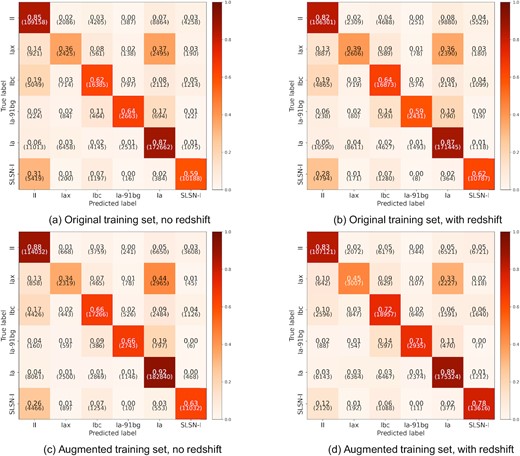
After training, all models were evaluated on the test set. Fig. 10 shows the confusion matrices for the models trained without transfer learning, using the original and augmented training set, with and without redshift information. Looking at the confusion matrices for the original training set, the model achieves good accuracy (|$\gt 80{{\ \rm per\ cent}}$|) for type Ia and II supernovae, a medium level of accuracy for type Ibc, Ia-91bg, and SLSN-I (|$\gt 60{{\ \rm per\ cent}}$|), and poor accuracy for type Iax supernovae. The biggest sources of confusion are type Iax and Ia-91bg being misclassified as Ia, and type Iax, Ibc, and SLSN-I being misclassified as type II. When redshift information is included, there is no major sign of improvement in performance.
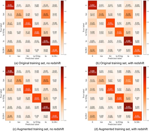
Confusion matrices for models without transfer learning (trained only on the PLAsTiCC data set), evaluated on the test set.
When the augmented training set is used, there is a slight improvement in accuracy for type II supernovae (and increase of |$\sim 7{{\ \rm per\ cent}}$| in accuracy), but no major change in performance in the other classes. Including redshift information does not have any significant improvement over the model without redshift information. There is an increase in the number of type Iax being misclassified as type Ia, and fewer SLSN-I being classified as type II.
7.2 Models with transfer learning
Fig. 11 shows the confusion matrices trained with transfer learning, using the original and augmented training set, with and without redshift information. For models trained on the original training set, both have slightly overall better performance over the same models without transfer learning, with an increase in accuracy by a few per cent across most classes, and fewer misclassifications. When including redshift, there is no significant improvement in performance.
Confusion matrices for models with transfer learning (using models trained on the Open Supernova Catalog data set and then fine-tuned to the PLAsTiCC data set), evaluated on the test set.
Looking at the models trained with the augmented training set, the performance for the model without redshift information is similar to the performance for the same model without transfer learning. When redshift information is included, the performance of the model with transfer learning is improved over the same model without transfer learning. There is good accuracy for type Ia and II supernovae (|$\gt 80{{\ \rm per\ cent}}$|), and improved accuracy for type Ibc, Ia-91-bg, and SLSN-I (|$\gt 70{{\ \rm per\ cent}}$|). There are fewer misclassifications overall (|$\lt 15{{\ \rm per\ cent}}$|), and the model trained with transfer learning and redshift information achieves the best accuracy out of all models on type Iax (|$45{{\ \rm per\ cent}}$|). We plot the difference between the confusion matrices for the models trained with transfer learning and without, for the augmented training set with redshift in Fig. 12, to illustrate the change in performance between the two models.
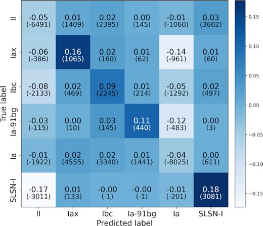
The difference between the confusion matrix for models trained on the augmented training set with redshift for with and without transfer learning. Positive values along the diagonal indicate an improvement when transfer learning is used. Negative values in the off diagonals indicate fewer misclassifications.
Table 6 shows the area under the receiver operating characteristic curve (AUC) score and the F1 score for all trained models, averaged across five different runs with the mean and standard deviation shown. The Hand & Till (2001) formulation is used to obtain the multiclass AUC scores presented in Table 6. In both cases with models trained with and without transfer learning, including redshift yields an improvement in the AUC score, but not always an improvement in the F1 score. A higher AUC score indicates that the model is able to produce fewer false positives, so when redshift is included the models are able to make predictions that have slightly less contamination at the small cost of not correctly classifying all true positive samples in each class.
AUC and F1 scores given as mean and standard deviation across five runs, trained on the original and augmented training sets with and without redshift, for both with and without transfer learning.
| Model | AUC | |$\pmb {\mathrm{F}_{1}}$| | |
|---|---|---|---|
| No transfer learning | Original, no redshift | 0.891 ± 0.005 | 0.618 ± 0.005 |
| Original, with redshift | 0.894 ± 0.004 | 0.59 ± 0.02 | |
| Augmented, no redshift | 0.923 ± 0.001 | 0.677 ± 0.003 | |
| Augmented, with redshift | 0.923 ± 0.003 | 0.651 ± 0.006 | |
| With transfer learning | Original, no redshift | 0.901 ± 0.002 | 0.615 ± 0.004 |
| Original, with redshift | 0.915 ± 0.001 | 0.607 ± 0.009 | |
| Augmented, no redshift | 0.924 ± 0.002 | 0.681 ± 0.001 | |
| Augmented, with redshift | 0.946 ± 0.001 | 0.660 ± 0.006 |
We also examine how selecting a threshold for class membership reduces the number of false positives in each class. Since the model makes predictions by producing a list of scores that represent how likely an object belongs to a specific class, we can define a threshold score so that if the score is above the threshold then the object belongs to that class, and if it is below then it is considered to not belong to that class. Three threshold values are selected: 0.5, 0.7, and 0.9. We consider the model trained with transfer learning using the augmented training set and redshift information. For each threshold value, any predictions that are below the threshold are excluded (looking at the highest score out of the six classes). For the following results, we consider results from a single run of models. Table 7 lists the AUC score, F1 score, and the fraction of samples retained at the different threshold values. Fig. 13 shows the confusion matrices for thresholds at 0.7 and 0.9. As the threshold value increases, the AUC score and F1 score improves but the fraction of samples retained decreases.

Confusion matrices for the model with transfer learning, trained on the augmented training set with redshift at different thresholds.
AUC and F1 scores for the transfer learning model trained on the augmented training set with redshift, evaluated at different probability thresholds. The column on the right shows the fraction of the test set retained when discarding predictions that are below the threshold.
| Threshold | AUC | |$\pmb {\mathrm{F}_{1}}$| | Fraction retained |
|---|---|---|---|
| 0.5 | 0.950 | 0.684 | 95.6 per cent |
| 0.7 | 0.960 | 0.752 | 83.2 per cent |
| 0.9 | 0.971 | 0.838 | 65.7 per cent |
| Threshold | AUC | |$\pmb {\mathrm{F}_{1}}$| | Fraction retained |
|---|---|---|---|
| 0.5 | 0.950 | 0.684 | 95.6 per cent |
| 0.7 | 0.960 | 0.752 | 83.2 per cent |
| 0.9 | 0.971 | 0.838 | 65.7 per cent |
7.3 Limited training set performance
To further investigate the impact transfer learning would have at the start-up phase of a new survey (i.e. when there is a very small sample of labelled data), we compare the classification performance of models with and without transfer learning when trained on 10, 25, and 50 per cent of the original PLAsTiCC training set. In this investigation, we consider a single run for each model configuration. Table 8 shows the AUC and F1 scores for these models, when trained with and without redshift information.
AUC and F1 scores, for models trained on different fractions of the original PLAsTiCC training set with and without transfer learning.
| Model | AUC | |$\pmb {\mathrm{F}_{1}}$| | |
|---|---|---|---|
| With transfer learning | 50 per cent of original, no redshift | 0.888 | 0.582 |
| 50 per cent of original, with redshift | 0.899 | 0.577 | |
| 25 per cent of original, no redshift | 0.869 | 0.574 | |
| 25 per cent of original, with redshift | 0.884 | 0.573 | |
| 10 per cent of original, no redshift | 0.827 | 0.520 | |
| 10 per cent of original, with redshift | 0.844 | 0.510 | |
| No transfer learning | 50 per cent of original, no redshift | 0.880 | 0.604 |
| 50 per cent of original, with redshift | 0.892 | 0.600 | |
| 25 per cent of original, no redshift | 0.880 | 0.579 | |
| 25 per cent of original, with redshift | 0.890 | 0.577 | |
| 10 per cent of original, no redshift | 0.836 | 0.513 | |
| 10 per cent of original, with redshift | 0.832 | 0.523 |
From Table 8, we can see that the AUC and F1 scores improve with an increased training set size for both with and without transfer learning. Overall, including redshift information improves performance across all models. An interesting point is that when no transfer learning is used, classification performance remains comparable to when transfer learning is used, and models trained on 50 per cent of the original training set shown an increase in F1 score with transfer learning compared to when no transfer learning is used.
To see how transfer learning impacts classification for individual supernova classes, we plot how the accuracy varies for each class as a function on training set size with and without redshift information in Fig. 14. All models achieve the best accuracies for Type Ia and Ibc supernovae, and the worst accuracy for Type Iax. There is no significant improvement in performance across all classes when transfer learning is used compared to training on the original PLAsTiCC training set alone. What is notable is that for type Iax and Ia-91bg, the classification accuracy is worse with transfer learning at smaller training set sizes. This could be due to the fact that the Open Supernova Catalog data contains many type Ia examples, and there is a small number of Type Iax and 1a-91bg examples in the PLAsTiCC training set. We also see that as the PLAsTiCC training set grows, the accuracy for Type Ia degrades while the accuracies for all other classes improve. This may arise from the fact that as the number of examples from non-Ia classes increases, the model learns to better classify non-Ia supernovae at the cost of misclassifying some Type Ia supernovae.
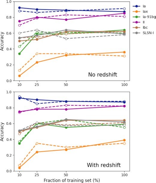
PLAsTiCC test accuracies across the six classes for different fractions of the original PLAsTiCC training set. The solid lines indicate accuracies for models with transfer learning and the dashed lines indicate accuracies for models without transfer learning.
8 DISCUSSION AND CONCLUSIONS
8.1 Classifying supernovae from multiple surveys
In order to classify the heterogeneous supernova light-curve data set, we use a 2D Gaussian process to model the light curves, and create a flux heatmap image for each light curve where each pixel in the image represents flux, as a function of time and wavelength. We also show that in the case where a supernova has good photometric coverage in multiple filters (measuring the flux at different wavelengths), the Gaussian process can be used to generate a low-resolution spectra of the supernova. Comparing the real spectra and Gaussian process generated spectra of supernova iPTF13bvn, we find that the two are comparable and the generated spectra does resemble the real spectra. It is not guaranteed, however, that all supernovae will have the same quality of photometric observations. Out of the original ∼80 000 supernova light curves from the Open Supernova Catalog, only 6330 were used to generate flux heatmaps with a 2D Gaussian process after selection cuts. A larger sample could be used, but at the cost of lower quality light curves (i.e. poor sampling in time and lack of multicolour observations), which may result in poor fitting with Gaussian processes.
We used a convolutional neural network to classify the supernova flux heatmaps, since the data are in a grid format that is well suited for the convolution operations carried out in the neural network. The model is able to classify Type Ia and II supernovae with good accuracy, but the class imbalance in the data set presents a challenge for classifying Type Ibc supernovae, since it is the class with the smallest number of samples and is not well represented in the training set. Deep learning approaches benefit from having a large data set to learn from, and we note that the Open Supernova Catalog data set is rather small for a deep learning application with less than 4000 samples in the training set. A future work may benefit from using a larger training set using flux heatmaps generated from simulated supernova light curves. It may also be interesting to investigate how the number of filters in a light curve (i.e. wavelength coverage) affects the flux heatmap.
8.2 Transfer learning for future surveys
We used a subset of 397 990 supernova light curves from the PLAsTiCC data set (The PLAsTiCC Team 2018), and use the 2D Gaussian process to generate flux heatmaps from the light curves. For the PLAsTiCC data set, we split the data into six classes, presenting a different classification task than the one for the Open Supernova Catalog data set. The original training set (containing 2398 SNe) and an augmented training set (containing 14 914 SNe) are used. Typically in most machine learning and deep learning methods, the training set is larger than the test set. Here, we use training sets that are much smaller than the test set to emulate the case where there is a scarcity of labelled data (the training set) and a large amount of unlabelled data (the test set).
In Section 7, we demonstrate that it is possible to transfer knowledge between two different domains (Open Supernova Catalog data and PLAsTiCC data) and two different classification tasks (three classes to six classes). The use of transfer learning shows a small improvement over when no transfer learning is used (and the model is only trained on the PLAsTiCC training set). We find the best increase in performance comes when redshift information is included and the augmented training set is used. It is possible to obtain better classifications with fewer misclassifications between classes when a threshold is used to remove ‘unconfident’ classifications provided by the classifier. Looking at the impact transfer learning has when there is a small labelled training set, we find that there is a slight improvement for well-sampled classes (e.g. Type Ia and II supernovae), but it provides no benefit for classes that have very few examples. Comparing the classification for Type Ibc supernovae for the PLAsTiCC data set and the Open Supernova Catalog data set, we see that the models achieve better accuracies with PLAsTiCC. This may be due to artificially less heterogeneity in the Type Ibc class in the PLAsTiCC data set. Kessler et al. (2019) note that in creating simulated light curves for Type Ibc supernovae for the PLAsTiCC data set, only a few dozen well-sampled light curves were used to develop the models used to generate Type Ibc light curves.
A limitation of the 2D Gaussian process approach used in this work is the requirement for sufficiently good coverage across multiple photometric bands and also in time. For future surveys such as LSST, this is dependent on the choice of observing strategy to provide a good enough cadence and wavelength coverage. The use of a 2D Gaussian process also relies on the full supernova light curve to create a good flux heatmap representation, which is still useful for the retrospective classification of supernovae to create samples for population studies. Stevance & Lee (2022) present a study on how Gaussian processes are used for modelling supernova light curves, and conclude that they are not well suited for this task since the kernels used are unable to accommodate a length-scale that varies with time. Supernovae behave on different time-scales in early times than at late times due to the radioactive decay of different elements. Alternative approaches will need to take into account the physics of supernovae and the varying time-scales involved.
In this paper, we present an approach to classify Open Supernova Catalog light curves from multiple surveys with a convolutional neural network by using a 2D Gaussian process to generate an image representation of supernova light curves. We find that using this method achieves good classification when there is good representation of the data in the training set. In the case of Type Ibc classification, the performance is poor since there is a lack of representation of Type Ibc supernovae in the training set. For classification tasks, it is important to have a good representative training set with good coverage in feature space for all classes so that a model is able to learn the feature–class relationship to make robust classifications.
We then investigate the usefulness of transfer learning in the context of future surveys where there may be a lack of labelled data to form a training set with which to train classifiers. The use of transfer learning shows a small improvement in classifiers compared to when no transfer learning is used when classifying PLAsTiCC supernova light curves. The addition of contextual information such as redshift and an augmented training set provided the best improvement in classification performance, highlighting the importance of a representative training set and the benefits of incorporating contextual information when classifying light curves. In the case of using transfer learning when there is a very small labelled training set, it may be useful to adapt a model that has been trained on a representative training set to account for class imbalance.
The methods presented in this paper could also be extended to classifying light curves of other non-supernova objects (such as variable stars, flare events, and AGNs). The flux heatmaps generated with the 2D Gaussian process could be used with a different neural network architecture such as a recurrent neural network, where each the input at each time-step is a single column of the heatmap representing the flux interpolated along wavelength. This would allow classifications to be obtained with time, and also be used to classify partial light curves (unlike the full light curves used in this paper), where the Gaussian process is used to interpolate the light curves up to the most recent observation as in Qu & Sako (2021).
A classification model that is agnostic to the different filters used across different surveys would be useful in the near future of time-domain astronomy. New objects observed by surveys such as LSST with the Vera Rubin Observatory could trigger follow-up observations by various instruments worldwide, which could be ingested by such a model to provide fast early time classifications to identify good candidates for time-sensitive observations.
Acknowledgement
The research of UFB and JRM was funded through a Royal Society PhD studentship (Royal Society Enhancement Award RGF\EA\180234) and STFC grant ST/V000853/1,respectively.
DATA AVAILABILITY
The work presented in this paper makes use of publicly available data from the Open Supernova Catalog (https://github.com/astrocatalogs) and the unblinded PLAsTiCC Classification Challenge data set (http://doi.org/10.5281/zenodo.2539456).
Footnotes
References
APPENDIX A: MAGNITUDE CONVERSIONS
Conversions between Swift magnitudes, Vega magnitudes, and the Carnegie Supernova Project (CSP) magnitude system into AB magnitudes are showin in Tables A1, A3, and A3.
Conversion table for Swift magnitudes given in the Vega system into AB magnitudes, obtained from Breeveld et al. (2011).
| Filter | AB – Vega |
|---|---|
| V | −0.01 |
| B | −0.13 |
| U | + 1.02 |
| UVW1 | + 1.51 |
| UVM2 | + 1.69 |
| UVW2 | + 1.73 |
| Filter | AB – Vega |
|---|---|
| V | −0.01 |
| B | −0.13 |
| U | + 1.02 |
| UVW1 | + 1.51 |
| UVM2 | + 1.69 |
| UVW2 | + 1.73 |
Conversion table for Vega magnitudes into AB magnitudes, obtained from Blanton & Roweis (2007).
| Filter | AB – Vega |
|---|---|
| U | 0.79 |
| B | −0.09 |
| V | 0.02 |
| R | 0.21 |
| I | 0.45 |
| u | 0.91 |
| g | −0.08 |
| r | 0.16 |
| i | 0.37 |
| z | 0.54 |
| J | 0.91 |
| H | 1.39 |
| Ks | 1.85 |
| Filter | AB – Vega |
|---|---|
| U | 0.79 |
| B | −0.09 |
| V | 0.02 |
| R | 0.21 |
| I | 0.45 |
| u | 0.91 |
| g | −0.08 |
| r | 0.16 |
| i | 0.37 |
| z | 0.54 |
| J | 0.91 |
| H | 1.39 |
| Ks | 1.85 |
Conversion table for magnitudes given in the CSP system into AB magnitudes, obtained from Krisciunas et al. (2017).
| Filter | AB - CSP |
|---|---|
| u | −0.06 |
| g | −0.02 |
| r | −0.01 |
| i | 0.00 |
| B | −0.013 |
| V | −0.02 |
| YRC | 0.63 |
| J | 0.90 |
| HRC | 1.34 |
| YWIRC | 0.64 |
| JWIRC | 0.90 |
| HWIRC | 1.34 |
| Filter | AB - CSP |
|---|---|
| u | −0.06 |
| g | −0.02 |
| r | −0.01 |
| i | 0.00 |
| B | −0.013 |
| V | −0.02 |
| YRC | 0.63 |
| J | 0.90 |
| HRC | 1.34 |
| YWIRC | 0.64 |
| JWIRC | 0.90 |
| HWIRC | 1.34 |
APPENDIX B: TRANSFER LEARNING TRAINING
Fig. B1 shows the training and validation loss for models trained without transfer learning, and Fig. B2 shows the training and validation loss for models trained with transfer learning. From these figures, it can be seen that 500 epochs is sufficient for the models to converge. The models trained on the augmented training set without transfer learning suffer from overfitting, where the validation loss begins to increase as the training loss continues to decrease.
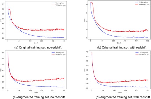
Training and validation loss during training for models without transfer learning.
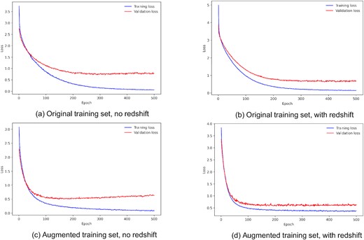
Training and validation loss during training for models with transfer learning.
