


ABSTRACT
We report the first simulations of planetary system dynamics as affected by an embedded cluster environment. Such environments are generally believed to be relevant for the large majority of newborn stars of solar type. Moreover, our cluster model is more realistic than in previous work. We focus on a giant planet system with five members, which represents a likely precursor of our solar system. Our main result is that the perturbing effects of close encounters with cluster stars trigger dynamical chaos leading to breakdown of the system with a significant probability, especially if the natal gas discs are short-lived and the clusters are highly concentrated. When breakdown occurs, all planets except Jupiter suffer a large risk of being ejected from the system or extracted into distant orbits with semimajor axes of hundreds or thousands of astronomical units. This is consistent with recent estimates of a large abundance of low-mass, free-floating planets. We demonstrate a possibility for Jupiter and Saturn to evolve into hot Jupiter orbits by tidal circularization during the chaotic evolution. Even so, the low occurrence rate of this outcome indicates that the real hot Jupiters in general have an origin unrelated to dynamical evolution in birth clusters.
1 INTRODUCTION
The majority of star formation occurs in associations generally known as embedded clusters (Lada & Lada 2003). Hence, only a minority of stars form in dynamical isolation, while most stars spend their infancy in embedded clusters. This begs the question on what influence this dynamical environment has on the newborn planetary systems. Specifically, does the dynamical influence of the cluster pose a threat to the stability of multiresonant giant planet systems as these emerge from the dissipating gas discs? This issue forms the scope of this paper.
An important motivation for the work is the fact that exoplanet systems are characterized by higher eccentricities than those of the solar system. In general, they have fewer planets and higher values of the NAMD (Normalized Angular Momentum Deficit) than the solar system (Turrini, Zinzi & Belinchon 2020). Such orbital architectures are at odds with the coplanar and nearly circular orbits expected for the abovementioned, newborn systems, indicating dynamically triggered breakdowns of this regularity (e.g. Rasio & Ford 1996; Weidenschilling & Marzari 1996). In principle, the trigger may be either internal to the system itself or external due to the dynamical environment.
The possible importance of the latter has been realized ever since the era of exoplanet discoveries started in the mid-1990’s. A recent review of the literature is given by Parker (2020). Among early papers addressing the issue we mention Laughlin & Adams (1998), where the authors estimated the likelihood of extremely close stellar encounters occurring in the birth clusters with the potential of directly disrupting the orbits of Jovian planets. They concluded that this outcome occurs frequently. Prompted by the preliminary detection of free-floating planets in the globular cluster M22 (Sahu et al. 2001), Hurley & Shara (2002) simulated the evolution of rich stellar clusters for the age of the solar system, finding the escape of planets – typically in wide orbits – to occur as a result of stellar encounters. These escapees were shown to stay as cluster vagabonds for time-scales comparable to the half-mass relaxation time.
Using the same concept of single planet systems, progress in the theoretical understanding of how such systems evolve under the influence of stellar encounters in clusters was achieved, for instance, by Bonnell et al. (2001) and Fregeau, Chatterjee & Rasio (2006). Their results were partly supported by numerical simulations. Multiplanet systems were first considered by Zakamska & Tremaine (2004), who studied the excitation of eccentricities in the outer parts of a planetary disc by very close stellar encounters and the subsequent, inward propagation of this eccentricity through a multiplanet system by orbital perturbations. They indicated that the mechanism offers a way to explain the elevated eccentricities of exoplanet orbits. Malmberg, Davies & Chambers (2007) concluded that exchange encounters in clusters may lead to the breakdown of multiplanet systems. The mechanism that they identified is that a single host star is captured into a binary during such an encounter, and the orbit of this binary has a high inclination to the plane of planetary motion so that the binary component excites Kozai oscillations of eccentricity and inclination, in particular for the outermost planet, leading to orbit crossing and close planet–planet encounters.
Spurzem et al. (2009) discussed another possibility for breakdown of a multiplanet system in a cluster environment. This involves close encounters experienced by the host star, which raise the eccentricity of a planetary orbit. The authors note that this may induce dynamical instability in closely packed planetary systems. However, their simulations did not provide direct evidence for the proposed mechanism, since only single (or otherwise unperturbed) planets were treated. Real evidence was found by Malmberg, Davies & Heggie (2011) through N-body simulations of open clusters. These had lifetimes of 400–1100 Myr. Attention was focused on fly-bys, where a solar mass star experienced a stellar encounter to within 1000 au. It was shown that the giant planets of the current solar system would stand a significant chance of being perturbed by such fly-bys to an extent that causes the ejection of at least one planet from the system. Importantly, these ejections often resulted from the internal, long-term dynamical evolution of the planetary system following the encounters. The planetary system used was modelled on the giant planets of the current solar system and thus not closely packed.
Hao, Kouwenhoven & Spurzem (2013) derived encounter frequencies from open cluster models and studied the effect of encounters within |$1\, 000\,\,$| au on planetary systems of two kinds orbiting around a solar mass star. In one case, five planets of jovian mass are separated by 10 Hill radii with semimajor axes of 1, 2.6, 6.5, 16.6, and 42.3 au. The other case involves the four giants of the current solar system on their actual orbits. As a general result, the outermost fictitious planet is mostly destabilized while the three innermost ones tend to be stable, and for the solar system only Jupiter remains stable. Kaib, Raymond & Duncan (2013) instead focused on planetary systems, whose host star is part of a wide binary, and showed such systems to be unstable to perturbations by the binary component as the binary properties change due to Galactic perturbations on Gyr time-scales.
A fundamental, statistical study of the effects of stellar encounters on planetary systems was published by Li & Adams (2015). Using over two million scattering simulations involving different cluster models and systems of four planets, the authors explored the dependence of the encounter cross-section for different planetary end states on cluster velocity dispersion, stellar host mass, and the starting radius and eccentricity of the planetary orbit. Cai et al. (2017) simulated the dynamical evolution of systems of five planets for 50 Myr in clusters with |$2\, 000$|, |$8\, 000$|, and |$32\, 000$| stars – all with the same virial radius of 1 pc. The planetary systems were of the fictitious kind studied by Hao et al. (2013) with an interplanet spacing of 10 Hill radii, and the clusters were initialized using the Plummer model in virial equilibrium neglecting binaries or mass segregation. The authors concluded that the systems are generally quite stable with fractions of lost planets increasing from ∼4 per cent for the least dense and rich clusters to values ∼5–10 times larger for the densest and richest clusters. More recent simulations by Flammini Dotti et al. (2019) focused on planetary systems modelled on the current solar system using clusters similar to those of Cai et al. (2017) though sometimes slightly subvirial or supervirial. In the course of 50 Myr, less than ∼5 per cent of the planets escaped – mostly those representing Uranus or Neptune. The resulting planetary systems were highly diverse in accord with what is seen for observed exoplanet systems.
Motivated by the conspicuous lack of confirmed exoplanets in globular clusters, Cai et al. (2019) simulated the dynamics of planets in a simplified model of a young massive cluster (YMC) possibly representing the precursor of Westerlund-1 using |$128\, 000$| stars. The planetary systems were either mass-less (thus excluding internal interactions) with semimajor axes from 6 to 400 au or comprised of five planets, each having three Earth masses, initially spaced between 0.5 and 6 au with a spacing of 15 Hill radii. In both cases the orbits were circular and coplanar. While most planets that start with semimajor axes beyond 20 au are ejected within 10 Myr, the majority that start within 5 au remain bound after 100 Myr.
Li, Mustill & Davies (2019, 2020) studied the effects of extremely close stellar encounters (pericentre distance <100 au), which stand a non-negligible likelihood of occurring for solar mass stars in typical open clusters, either immediately by direct impulses to the orbiting planets or by the long-term evolution of the perturbed planetary system. In one case (Li et al. 2019) the initial system was modelled on the solar system, while in the other case (Li et al. 2020) the planetary systems were different and sometimes modelled on observed exoplanet systems.
van Elteren et al. (2019) simulated the dynamical evolution of planetary systems placed within the Orion Trapezium cluster. These systems were modelled on the circumstellar disc size distribution derived for this cluster by Portegies Zwart (2016), and the cluster model was substructured with a fractal dimension of 1.6. The planetary systems contained four, five, or six, on average Saturn-sized, planets on initially circular and coplanar orbits. The simulations were extended for a period of 11 Myr. The results were focused on the production of free-floating planets, and the two basic mechanisms were found to be direct impulses due to strong stellar encounters or the subsequent, internal planetary scattering.
Stock et al. (2020) performed simulations to explore the way cluster perturbations influence the evolution of planetary systems using the four solar system giants as models. The clusters had from |$8\, 000$| to |$64\, 000$| members initialized as Plummer spheres without substructure, and the planetary systems were integrated for 100 Myr considering the five closest stars as perturbers. The initial system architectures were the same as used by Li & Adams (2015) including the current solar system orbits plus more compact configurations including a multiresonant case. As a general result, the systems proved quite resilient to the cluster perturbations.
In a recent study, Daffern-Powell & Parker (2022) investigated two special phenomena caused by the influence of close stellar encounters in a cluster on planetary systems. One is planet stealth, where a planet gets released from its previous host star and gets bound to the intruder. The other is planet capture, where a free-floating planet emanating from an ejection during a close encounter becomes gravitationally bound to another star at a second close encounter. To this end, simulations of substructured, young clusters were carried out for 10 Myr in subvirial or supervirial states, and the planets were put on circular orbits around their host stars or made free-floating. Comparison of the orbital properties of stolen, captured, or preserved planets indicated the possibility of distinguishing between the different modes of origin of observed exoplanets.
It has repeatedly been pointed out that the relative scarcity of exoplanets in stellar clusters indicates that such planets have been lost due to dynamical processes characteristic of such clusters (e.g. Spurzem et al. 2009; Stock et al. 2020). Such losses may have occurred in the presently observed clusters or in their very young precursors, i.e. embedded clusters. Related to this, Winter et al. (2020) presented evidence that the host stars of hot Jupiters belong to overdense regions in the phase space of the Galactic disc in a way that strongly suggests an origin triggered by external perturbations. Turrini et al. (in preparation) have provided a comprehensive analysis of observational data on the excitation of exoplanet systems and a discussion of underlying effects of both internal and external nature.
While many interesting results have been obtained for planetary systems affected by the typical environments of open or globular clusters, as described above, these only pertain to a minority of the solar-type stars at large because of the well-known ‘infant mortality’ problem: the initial associations only rarely develop into such long-lived clusters (e.g. Elmegreen & Clemens 1985; for a recent discussion see Wiśniowski, Rickman & Wajer 2021). Most stars have only experienced the environment of their embedded birth clusters for the short time until these were dispersed.
Consequently, in this paper, we turn our attention to the embedded clusters using a novel modelling scenario. Our work differs from all previous papers in that, simultaneously, (1) we use cluster models that, by introducing early gas release, are consistent with the short lifetimes of most birth associations; (2) we explicitly simulate the evolution of the planetary system as a consequence of the full cluster evolution without limiting ourselves to any special features; (3) we select a realistic model of a newborn, multiresonant giant planet system as predicted by migration models of planet formation. We use a new model for simulating circumstellar dynamics in young clusters (Wiśniowski, Rickman & Wajer 2022), and our standoff planetary system is taken from the work of Nesvorný & Morbidelli (2012) as a possible precursor of our solar system in the framework of the Nice Model.1 Our cluster model is homogeneous. Several previous papers on the stability of newborn planetary systems (e.g. Parker & Quanz 2012; Craig & Krumholz 2013; Zheng, Kouwenhoven & Wang 2015) have focused on substructured, young clusters and compared the encounter rates with those of corresponding, homogeneous models, and we shall return to this in Section 4.
In Section 2 we provide a detailed description and discussion of our modelling techniques and computational strategy, and our results will be presented in Section 3. Section 4 is devoted to a discussion of our results and their implications, and we conclude in Section 5.
2 COMPUTATIONS
2.1 Cluster simulations
The basis for our computations is a set of numerical models for embedded clusters that evolve from an initial structure taken to be a Plummer sphere over a time interval of 10 Myr. These have been described in detail by Wiśniowski et al. (2021, 2022) and here we only summarize a few important aspects. Our N-body simulations were made using the nbody6++gpu code (Wang et al. 2015), which is a modern implementation of the nbody6 package (Aarseth 2003). Because of our inclusion of an external tide due to a nearby clump in the surrounding GMC, the resulting evolutions are broadly consistent with observations regarding the cluster lifetimes (Wiśniowski et al. 2021). Typically, the cluster starts by contracting due to the assumption of an initially subvirial velocity distribution. The following rebound is accelerated by the loss of gravitational potential as the placental gas becomes dispersed. This causes the loss of stars via the effect of the external tide.
All our models use the same number of initial stars (|$N_0 = 1\, 000$|), which we consider to be broadly representative of embedded clusters at large. We use the IMF of Kroupa (2001). Two parameters are varied. One is the degree of concentration of the initial Plummer sphere, for which we consider either a moderate value of the Plummer radius (1.17 pc) or half thereof (0.585 pc) indicating a high degree of concentration. The other is the delay time of gas loss (Brinkmann et al. 2017), for which we consider either a low value (0.6 Myr) based on the existence of very young, gas-free clusters (Banerjee & Kroupa 2013) or a value four times higher (2.4 Myr) being representative of what may be the majority of embedded clusters (Brasser et al. 2012).
Combining both values of both parameters, we obtain a set of four basic models. These are denoted by A and B for low concentration and C and D for high concentration. A and C clusters have a shorter gas lifetime and B and D a longer one. We have performed three random realizations of each of these, resulting in a set of 12 model clusters. In each of these we have selected six solar template stars, initially single with masses within 5 per cent of the solar mass and no other constraints. The resulting set of 72 stars displays a random set of cluster trajectories with a broad range of characteristics, for instance, as regards the number of close encounters or the minimum distance from the cluster centre.
Fig. 1 illustrates an important difference between the four cluster types regarding the strength and frequency of close encounters by plotting the masses and minimum distances of the stellar intruders in all the closest encounters with the most massive stars, experienced by the solar templates. For this purpose, we use the extreme cases of A and D clusters exhibiting the smallest and largest encounter frequencies, respectively.
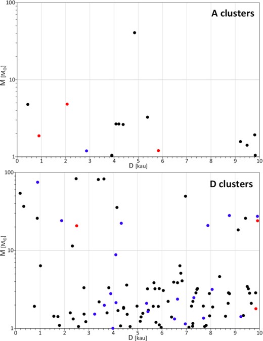
Masses versus minimum distances of stellar intruders for solar templates in A and D clusters. For binaries, the total mass and the distance of the centre of mass is used. The time of the encounters is marked by colours: black for times less than 2 Myr, blue for times between 2 and 5 Myr, and red for times larger than 5 Myr.
2.2 Planetary system simulations
In the next step, we have used the same 72 stars in numerical simulations of planetary system evolution under the influence of cluster effects during the 10 Myr interval of our cluster simulations. We now concentrate on the solar system, so we give each star the mass of 1.0 solar masses and let it be surrounded by a giant planet system representing a possible precursor of our solar system. For the latter we use initial parameters taken from the work of Nesvorný & Morbidelli (2012) – see Table 1. These correspond to a time, when the solar nebula had dissipated and the planets moved under the influence of gravity alone including that of the Sun, those of themselves, and those caused by the scattering of trans-Neptunian planetesimals at close encounters. In the simulations by Nesvorný & Morbidelli (2012), the latter caused a chaotic period with multiple planet–planet encounters representative of the Nice Model, eventually leading to a system consistent with the present solar system.
Starting conditions for the planetary system given as orbital elements referred to the invariant plane. Masses are given in units of 10−4 M⊙.
| Planet | Mass | a (au) | e | i (○) | Ω (○) | ω (○) |
|---|---|---|---|---|---|---|
| Jupiter | 9.548 | 5.71 | 0.0034 | 0.013 | 356.3 | 331.3 |
| Saturn | 2.858 | 7.78 | 0.0115 | 0.062 | 8.3 | 124.2 |
| Planet 5 | 0.426 | 10.51 | 0.0037 | 0.090 | 35.5 | 94.6 |
| Uranus | 0.426 | 17.62 | 0.0022 | 0.032 | 351.2 | 166.2 |
| Neptune | 0.508 | 23.34 | 0.0018 | 0.067 | 75.0 | 266.4 |
In this work we neglect the influence of the planetesimals and replace it by the effects of the embedded cluster. The planetary system at hand involves five giant planets, where the four known ones are supplemented by a fifth planet, which was initially moving in an orbit between those of Saturn and Uranus with the typical mass of an ice giant and was later ejected during the chaotic period. Note that this system was chosen to be long-term stable barring the effects of the planetesimal disc, and thus we expect it to remain stable in our simulations unless the cluster effects induce an instability. This expectation was verified by actual simulations.
Our planetary system simulations have been made with two different N-body integrators: RA15 (Everhart 1985) and IAS15 (Rein & Spiegel 2015), using two different computers. The implementation of the cluster effects is identical in all cases. An important decision has to be made concerning the starting time of the simulations. For reference, we have made one set of simulations using a starting time equal to zero – however, this is unrealistic since we have to allow for the time to build the planets and for the solar nebula to dissipate. We refer to this delay as DT, and we have considered three values: 0, 2, and 5 Myr. Hence, all the 72 simulations are performed three times using the different DT values.
The cluster effects are of two kinds (Wiśniowski et al. 2022). On the one hand, the global potential field of the cluster causes a tidal force acting on the planets orbiting around the Sun. On the other hand, during close encounters with other cluster members (single stars, binaries, or temporary mergers between a binary and a single star) the intruder acts by its gravity, differentially, between the planet and the Sun. Our criterion for defining close encounters is much more liberal than that of Malmberg et al. (2011), since we consider all intruders passing within |$40\, 000\,\,$| au from the Sun. We note that, though the cluster tide is included in our computations, it is not expected to contribute significantly to the perturbations of the planetary orbits. When a nearly circular orbit around the Sun is described, the tidal accelerations of a planet nearly cancel out. Due to secular changes of the tidal strength, a cumulative effect appears over many orbits, but this does not compete with the effects of relatively strong encounters.
During periods of chaotic motion, extremely close encounters may occur. However, despite the fact that the equations of motion refer to point masses, infinite accelerations are avoided by a check against physical collisions. For this we use the actual equatorial radii of Jupiter, Saturn, Uranus, and Neptune, and we assume the fifth planet to have physical properties identical to those of Uranus. For the solar template star we use a value of |$700\, 000\,\,$| km. Needless to say, collisions can only occur in unstable systems. In case of a planet–Sun collision, the planet disappears while all the others continue as if nothing happened. However, the results of planet–planet collisions are unpredictable without detailed hydrocode modelling of those events, so the collisions are noted and the simulations are stopped.
2.3 Analysis
When analysing the results, we first observe the behaviour of the planetary semimajor axes. This can be of two kinds. In one case, the semimajor axes (a) remain essentially constant so that a panoramic diagram showing all of them against time from 0 to 10 Myr features a set of parallel, horizontal lines superposed by insignificant, short-term fluctuations. We call these systems stable. In the other case, we see sudden jumps, often involving ejections from the solar system or expulsions into long-period orbits, and we refer to this as breakdowns. Further analysis is required to reveal the mechanisms at work, and we shall describe this in Section 3.3.
3 RESULTS
3.1 Frequency of breakdowns
We shall now examine the distribution of the basic property of a planetary system: stability versus instability. Fig. 2 illustrates three typical behaviours. In panels (a) and (b) we see stable systems, and the difference is that system (a) is essentially unmodified in spite of the cluster interactions, while system (b) is clearly modified. In particular, Uranus and Neptune acquire orbits with significantly increased eccentricities. To a smaller extent, the same is true for all the other planets as well, and the reason is a close stellar encounter occurring after 0.68 Myr. This type of evolution dominates among the stable systems and unmodified systems are relatively rare.
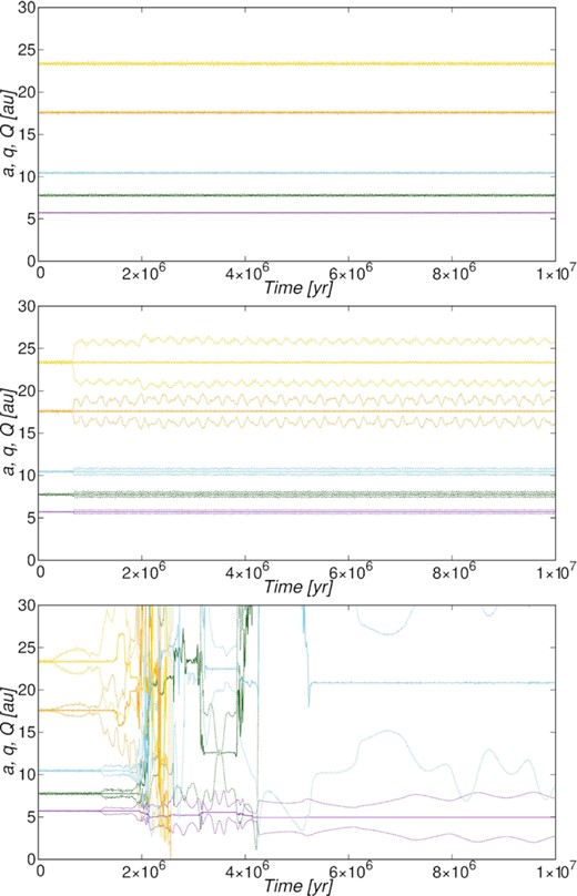
Perihelion distance q, semimajor axis a and aphelion distance Q of the five planets versus time according to three RA15 simulations with zero starting time. Full-drawn curves are used for the semimajor axes and dotted curves for the perihelion and aphelion distances. Jupiter is plotted in violet, Saturn in green, Planet 5 in blue, Uranus in orange, and Neptune in yellow. Panel (a) is shown on top, panel (b) in the middle, and panel (c) at the bottom.
Panel (c) shows a system that underwent a breakdown. The effects of stellar encounters are seen early on and, starting from about 1 Myr, a series of encounters with stellar binaries raise the eccentricities of Uranus and Neptune so that orbital crossing occurs. During this time, the solar template star moves close to the cluster centre in a high density environment. Close planet–planet encounters start occurring soon thereafter, leading to chaotic evolution of the system. The climax arrives after 2.6 Myr with a 4 M⊙ star passing very slowly at a minimum distance of about 860 au. As a result, Uranus and Neptune are ejected near 2.6 Myr and Saturn is extracted into an orbit with a ∼ 120 au after 4.1 Myr – all resulting from close encounters with Jupiter. Ejection of Planet 5 by such an encounter after more than 10 Myr seems likely.
In Table 2 we summarize the numbers and percentages of planetary systems that experienced breakdowns in simulations with the starting time chosen as 0, 2, and 5 Myr. The total number of simulations using RA15 or IAS15 integrators for any specific starting time is 144. Broadly speaking, the agreement between both integrators is very good. For the reference simulations with starting time set to 0, the only disagreement occurs in the B cluster, where one of the five unstable systems differs between the two. The disagreements are more common for the simulations with delayed starting time. For 2 Myr, one system in a D cluster is unstable only in the RA15 simulation, and for 5 Myr, the same holds for two systems: one in an A cluster and the other in a C cluster.
Numbers of simulations yielding unstable planetary systems, followed by the corresponding percentages within parentheses, listed separately for low and high concentration clusters and for the different starting times. By ‘DT’ we denote the delay of the simulation starting time in Myr.
| Clusters | DT = 0 | DT = 2 | DT = 5 |
|---|---|---|---|
| A,B | 20 (28 per cent) | 8 (11 per cent) | 5 (7 per cent) |
| C,D | 48 (67 per cent) | 25 (35 per cent) | 5 (7 per cent) |
| Clusters | DT = 0 | DT = 2 | DT = 5 |
|---|---|---|---|
| A,B | 20 (28 per cent) | 8 (11 per cent) | 5 (7 per cent) |
| C,D | 48 (67 per cent) | 25 (35 per cent) | 5 (7 per cent) |
We see a marked difference of these results between the low concentration clusters (A and B) and those of high concentration (C and D), the unstable cases being much more common for C and D clusters with starting times of 0 and 2 Myr, while this difference disappears when the starting time is 5 Myr. Noting that – beyond the scope of this paper – very early encounters may have profound effects on the gas discs out of which the giant planets are born (see Pfalzner et al. 2018), we emphasize that the remarkably high unstable fractions for DT = 0 are unrealistic and only serve for comparison. On the other hand, those listed for delay times of 2 or 5 Myr can be regarded as realistic and interpreted using the current observational evidence on gas disc lifetimes (see Section 4).
3.2 End states
It is of obvious interest to examine the properties of the planetary systems at the end of our simulations – in particular for the systems that experienced breakdowns. A rather frequent outcome is the extraction of one or more planets into very distant orbits, for which we shall adopt a definition of a > 100 au. In fact, individual cases scatter from just above this limit to tens of thousands of astronomical units. We thus classify the terminal orbits into three types: ejected, meaning a positive orbital energy (a < 0); extracted, meaning orbits bound to the solar system with a > 100 au; and remaining, which means bound orbits that stay with a < 100 au.
In addition, a small number of planets are physically destroyed by collisions – either with the Sun or with another planet. For these, the end state is classified as destroyed. In total, there were four planet–planet collisions, of which three involved Jupiter, and 12 Sun–planet collisions, of which only one involved Jupiter.
From the data presented in Section 3.1 it is clear that the RA15 simulations of the reference type with zero starting time yielded 34 cases of breakdown. To have a homogeneous sample, we only consider such simulations for studying the end state statistics. We also consider independent IAS15 simulations of the same cases, but these suffer from a problem apparently caused by the step size regulation technique adopted in this integrator (Rein & Spiegel 2015). This step size cannot exceed the minimum physical time-scale of the dynamics involved, and for extremely close encounters – such as near collisions between planets – the integration tends to slow down to the point where it becomes unmanageable. In six of the 34 cases we were thus unable to finish the IAS15 integrations. It was already clear that a breakdown had led to chaotic motion, but we could not establish the end states. Adding the 28 successful IAS15 simulations to those from RA15, we thus have a total of 62 sets of end states to analyse. When a planet–planet collision occurs, this set is incomplete involving only the two collision partners (see Section 2.2).
Naturally, different planets may prefer different end states, and in Table 3 we show these trends in terms of the occurrence rates of the four end states for all five planets. Jupiter stands out as by far the most stable planet, followed by Saturn with more than 60 per cent in the remaining category. Planet 5 has the largest fraction of ejections and the smallest chance to stay in the remaining category. Overall, we find that the ejections outnumber the extractions by about 50 per cent.
Numbers of end states, followed by the corresponding percentages within parentheses, as found from all the completed simulations of unstable systems with zero starting time.
| Planet | Ejected | Extracted | Remaining | Destroyed |
|---|---|---|---|---|
| Jupiter | 0 (0 per cent) | 0 (0 per cent) | 57 (93 per cent) | 4 (7 per cent) |
| Saturn | 9 (15 per cent) | 8 (14 per cent) | 39 (66 per cent) | 3 (5 per cent) |
| Planet 5 | 29 (49 per cent) | 16 (27 per cent) | 8 (14 per cent) | 6 (10 per cent) |
| Uranus | 22 (37 per cent) | 15 (25 per cent) | 17 (29 per cent) | 5 (9 per cent) |
| Neptune | 21 (35 per cent) | 13 (22 per cent) | 21 (35 per cent) | 5 (8 per cent) |
In Fig. 3 we show the distributions of final semimajor axes for Jupiter and Saturn as found in the simulations of unstable systems with zero starting time, where the planet belongs to the remaining category. The data are complete for Jupiter, while for Saturn we have disregarded one case where afin is close to 100 au. Here we see the effects of planet–planet encounters during the chaotic periods marking the breakdowns. Naturally, Jupiter is the hardest to move with its large mass, and for Saturn we mainly see the results of gravitational scattering by Jupiter.
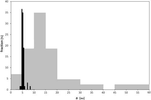
Histograms plot of the distributions of semimajor axes for Jupiter and Saturn at the end of our simulations. The grey shaded histogram refers to Saturn and the black histogram to Jupiter. Different bin sizes have been used. The sum of the percentages over all bins is 100 per cent for Jupiter and 98 per cent for Saturn, the histogram having been cut at a = 60 au.
In Table 4 we present our results for the final multiplicity of the unstable planetary systems in all the 58 relevant simulations. Of course, the initial multiplicity is always M = 5. Here we distinguish between two values: M1 includes all the planets that were not ejected or excluded by collision with the Sun, while M2 also disregards the extracted planets, thus counting only planets with afin < 100 au.
Number of planets (multiplicity) of the final, unstable planetary systems according to two definitions (see the main text for details).
| Multiplicity | 0 | 1 | 2 | 3 | 4 | 5 |
|---|---|---|---|---|---|---|
| M1 | 1 | 3 | 7 | 17 | 24 | 6 |
| M2 | 1 | 8 | 25 | 14 | 8 | 2 |
| Multiplicity | 0 | 1 | 2 | 3 | 4 | 5 |
|---|---|---|---|---|---|---|
| M1 | 1 | 3 | 7 | 17 | 24 | 6 |
| M2 | 1 | 8 | 25 | 14 | 8 | 2 |
This shows that, counting the extracted planets, more than half the final systems have at least four planets, while more than half have no more than two planets if the extracted planets are excluded.
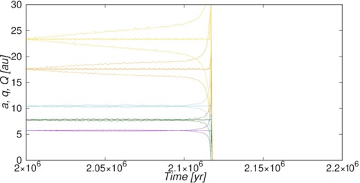
Our method of estimating NAMD works only for systems, where the simulation has reached the end state at 10 Myr. In case of a planet–planet collision or if the IAS15 simulation got stalled before the end, this is not the case and NAMD values are lacking. Otherwise, we use two somewhat different strategies. The one used for RA15 simulations is illustrated in Fig. 4. Here we calculate instantaneous values of NAMD throughout the simulation and use the final interval, where the oscillating NAMD values define a stable, constant, or slowly varying average. For the IAS15 simulations we instead take the average over the last 0.5 Myr, noting that reasonable stability is always present.
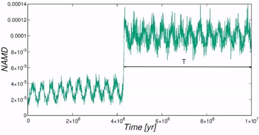
Instantaneous NAMD values plotted as a function of time for a system of remaining planets (a < 100 au) belonging to an A cluster. The system is stable with M2 = 5. The time interval marked ‘T’ is the one used to derive the final, average NAMD. The sudden change appearing in the NAMD evolution at the start of this interval is caused by a close encounter with a low mass binary star.
In Fig. 5 we present our resulting NAMD values separately for stable and unstable planetary systems. For the stable systems (Fig. 5a) we see a scatter from the initial NAMD of 2 × 10⁻⁵ up to values about 100 times larger due to the frequently occurring excitation of substantial eccentricities, in particular for Uranus and Neptune. The four largest values occur for systems where Uranus and Neptune end up on marginally crossing orbits, avoiding close encounters. The A system with the two largest values shows a more substantial excitation of the other planets than the two B systems. For the latter, by coincidence, the two simulations yield different results on stability.
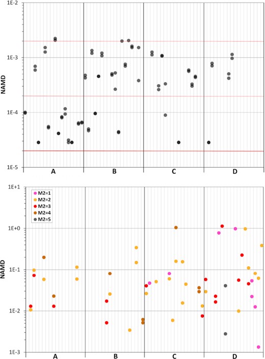
(a) Average NAMD characterizing the stable planetary systems, plotted separately for the different systems by filled dark grey circles. Wherever possible, both values from RA15 and IAS15 simulations are plotted. The horizontal red lines indicate the NAMD of the initial system (thick line) and values 10 times and 100 times larger. (b) The average NAMD of unstable planetary systems, plotted separately for the different systems. The colours of the filled circles denote the multiplicities (M2) as explained in the inserted legend. Like in panel (a), both RA15 and IAS15 simulations are represented. Panel (a) is shown above and panel (b) below.
In this case, the final NAMD distributions differ substantially between the different clusters. Values less than ten times the initial value dominate in numbers (10/3) over the larger values for the A clusters, while the B clusters show the opposite difference with the larger values in majority. A predominance of large values is also seen for the C and D clusters with a combined preference of 10/2 over the smaller values. This indicates that, for most embedded clusters, the stable planetary systems are typically left in a significantly excited state.
Fig. 5(b) shows quite a different distribution. Here the NAMD values range over three orders of magnitude between about 100 and |$100\, 000$| times the initial value. The A clusters show the smallest scatter of individual values. The D clusters exhibit practically all the extremely large values, almost 105 times larger than the initial NAMD. Judging from both panels together, it is obvious that there is practically no overlap of NAMD values between stable and unstable systems, implying that systems with multiplicity M2 = 5 have by far the smallest NAMD. However, concentrating on the unstable systems, a trend for lower multiplicity to correlate with larger NAMD (see Turrini et al. 2020), while being possible to trace, is practically drowned by the large scatter of NAMD for all M2 values.
The inclinations used in our definition of NAMD are referred to the invariable plane of the initial planetary system. This is necessary in order for the NAMD values to reflect the dynamical heating of the systems. To reach some insight into the respective roles of eccentricity and inclination in this heating, we have studied the distribution of cos i for all the individual planets under consideration. For simplicity, we have taken the instantaneous values at the end of the simulations after 10 Myr in all cases where these are available. In the two panels of Fig. 6 we show histograms of 1 − cos i, using a log scale, for planets in stable and unstable systems, respectively. For instance, the value 10−3 corresponds to i ≈ 2.56°.
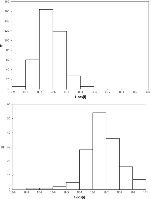
(a) Histogram distribution of the final values of cos i for planets in stable systems according to both RA15 and IAS15 simulations. (b) The same for planets in unstable systems. Panel (a) is shown above and panel (b) below.
For planets in stable systems with inclinations of a few degrees or less, the NAMD is essentially given by the final eccentricities. On the other hand, in unstable systems a fair fraction (∼20 per cent) have inclinations exceeding 26° and cos i < 0.9 so that the role of the inclinations in the NAMD may be significant. For the RA15 simulations, we have a total of ten planets with i > 60° (cos i < 0.5). As much as four of these cases involve Jupiter. The basic reason is scattering events at close planet–planet encounters, where Jupiter is frequently involved. We find only two cases of planets with significantly retrograde, final orbits (Uranus and Planet 5). We note that the final inclination values are not always stable but often represent patterns of secular oscillations with important amplitudes.
3.3 Breakdown mechanism
Unfortunately, it is not possible to uniquely establish the exact mechanism leading to breakdown by quantitative analysis for the individual simulations. We are limited to the use of diagrams like panel (c) of Fig. 1 by visual inspection and comparison with the lists of selected stellar encounters and plots of the tidal strength versus time. Moreover, the number of encounters is often large, since these tend to concentrate around the time periods when the central density of the cluster is maximal. The average number of encounters per template star is about 5, 8, 13, and 20 for the A, B, C, and D clusters, respectively, and there are large variations between individual templates in each case depending on the actual cluster orbits.
Nevertheless, qualitative indications easily stand out from the mentioned observations. One indication is the complete lack of evidence for breakdowns being triggered by the cluster tide, which confirms the expectation mentioned in Section 2.2. We also note that panel (a) of Fig. 2 illustrates one of the few cases where the template star had no encounter at all. In this case it is clear that the cluster tide had no visible effect. On the other hand, there is not a single breakdown that cannot be associated with one or more stellar encounters. These almost always have remarkably large values of the so-called strength parameter S (see Wiśniowski et al. 2022), indicating large impulses conveyed to the solar template and surrounding planets.
In principle, the differential effect of these impulses may be imagined to be so small that a planetary system already close to chaotic motion is perturbed into a new track leading into chaos only after a shorter or longer waiting time. However, we do not see this occurring. Instead, in the large majority of cases, we see the immediate effect of the encounter in an increase of the orbital eccentricities of Uranus and Neptune, as shown in panels (b) and (c) of Fig. 2. The trigger of chaos is the possibility of close encounters between these two planets – a possibility that is often realized quite soon. In such a case, the ensuing scattering tends to allow encounters with Planet 5, whereupon the chaos easily spreads to Saturn and Jupiter as well. We also note that direct ejections or extractions of planets by impulses deriving from stellar encounters are not seen except in one singular case.
This concerns one template star in a D cluster, which had an extremely strong encounter with a very massive binary (total mass of about 75 M⊙) after 2.1 Myr. The minimum distance was only about 900 au and the template star was nearly captured by this binary. In Fig. 7 we show the result of our RA15 simulation with a starting time delayed by 2 Myr. Obviously, all the planets (including Jupiter) were ejected almost simultaneously during this encounter, and the timing fits perfectly with the closest approach. Estimating the cumulative, heliocentric impulse of a planet by integrating equation (3) along a straight line trajectory of the binary until the time of closest approach, one finds that the combination of the components along and orthogonal to this line may be relevant to cause hyperbolic ejection of Jupiter and, slightly before this, of the other planets too. This is in accordance with the observed, detailed sequence of ejections.
Perihelion distance q, semimajor axis a, and aphelion distance Q of the five planets versus time according to our RA15 simulation with starting time at 2.0 Myr for a star in a D cluster undergoing an extremely strong encounter at 2.117 Myr (see the main text). For styles and colours of the curves, see the caption of Fig. 2.
From this investigation, the most outstanding features concern the mass and binarity. Among the triggering encounters, 78 per cent involve binaries, but only 41 per cent among the non-triggering ones. Masses larger than 10 M⊙ yield 58 per cent of the triggering encounters but only 16 per cent of the non-triggering ones. The preference for large masses is natural since this increases the strength S, but the preference for binarity may also involve an increased likelihood of stimulating breakdown by a binary system as compared to a single star. Concerning the minimum approach distances, we note some preference for values less than 10 kau among the triggering encounters, which is natural as these encounters tend to be the strongest ones. Concerning the velocity at infinity, we do not see any tendency for lower values among the triggering encounters, but it is worth noticing that about 90 per cent of these velocities are less than 5 km s−1 due to the cluster kinematics.
4 DISCUSSION
We shall now discuss the applicability and implications of the above results. Naturally, the lifetimes of gas discs in star-forming regions are an important issue. According to Meyer (2009; see also Hillenbrand 2008), the proportion of infant stars that are associated with gas discs decreases from 100 per cent to ∼30 per cent after 2 Myr and <10 per cent after 5 Myr. We take this to imply that the majority of the planetary systems that we investigate would experience higher breakdown rates than our results assuming DT = 2 Myr, and more than 90 per cent of such systems would experience higher breakdown rates than our results assuming DT = 5 Myr.
From the values listed in Table 2 we infer that planetary systems formed in clusters of relatively low density in most cases stand a chance of at least 11 per cent to experience cluster-induced breakdown, and in high density clusters this increases to 35 per cent. Independent of the type of cluster, the chance of such breakdown is less than 7 per cent in only ∼10 per cent of the cases. The fact that the breakdown rate differs considerably between high and low density clusters for DT ≤ 2 Myr but disappears for DT ≥ 5 Myr is most naturally interpreted by considering that the very high number densities characterizing the high density clusters only occur in the beginning of their evolution. On the other hand, the late breakdown-triggering encounters occur rarely and equally in both kinds of cluster.
At this point, a few comments must be added. Our results apply only to one type of initial planetary systems, namely, those that resemble a likely precursor of our solar system. It is impossible to say how frequent those systems are among all planetary systems formed in the Galaxy at present or in the past. However, it is clear that, practically, discovery selection forbids such systems to exist in the observed exoplanet data base. Since most observed systems are much smaller, these may much more often have broken down due to internal instabilities. This issue remains to be investigated.
It should also be noted that our breakdown rates are somewhat conservatively estimated, since we stopped our integrations and judged the stability of the planetary systems after 10 Myr. Hence, some of the systems judged to be stable may in fact break down at a later time, since Uranus and Neptune are left on crossing orbits. In general, the time scale for gravitational scattering between these planets in case of orbital crossing largely exceeds 10 Myr, but such scattering is hard to avoid given enough time, and the consequences would likely involve the other planets too. In addition, concerning the general applicability of the Nice Model scenario (Nesvorný & Morbidelli 2012), we note that among the undoubtedly stable systems there is a large fraction where significant eccentricities have been reached by Neptune and Uranus. From the time that these were excited, Neptune would likely have started scattering the objects of a hypothetical, trans-planetary disc, thus initiating its pre-migration phase. The times in question tend to be quite early.
Another important issue is to what extent our results are biased by our choice of cluster models. Clearly, the parameter space of cluster models has been very sparsely sampled, and the issue can only be treated in terms of educated guess. One parameter that was fixed for all models is the number of stars, |$N_0=1\, 000$|. Real embedded clusters range from N0 < 100 to |$N_0\sim 10\, 000$|. In this case we argue as follows. We have seen that breakdowns tend to be caused by close encounters, and the number of such encounters tends to increase with the stellar number density in the central parts of the cluster. This, in turn, is proportional to N0 suggesting that breakdowns are quite rare in the smallest clusters and quite frequent in clusters larger than we have considered. However, the concentration given by the Plummer radius plays a more important role – in the two kinds of cluster that we treat, the central density differs by almost a whole order of magnitude. Thus, we can make the general statement that the breakdown rates reported in this paper will be overestimated for very small clusters with low concentration and underestimated for rich and strongly concentrated clusters.
Our breakdown rates may have been generally underestimated for another reason, namely, that we use a homogeneous cluster model neglecting the likely presence of substructure. This is because the stars would tend to reside in high-density filaments, where the encounter rate is boosted with respect to the homogeneous average (see Parker 2014). Parker & Quanz (2012) modelled the evolution during 10 Myr of a single, Jupiter mass planet orbiting at 5 au in subvirial clusters with fractal dimension D = 2 and |$1\, 500$| stars. They found a 5 per cent probability for this planet to be ejected, while in our case Jupiter was never ejected or extracted. However, this may be due to our small sample of 72 planetary systems, where 5 per cent would only mean 3–4 ejections. Moreover, the clusters of Parker & Quanz (2012) are somewhat larger than ours and unaffected by gas loss leading to early dispersal. Craig & Krumholz (2013) noted that the boosting of encounter rates in high-density filaments is just a transient phenomenon lasting for about one crossing time before the filaments are erased by dynamical interactions. In their short-term simulations, planetary systems were found to be remarkably stable against stellar encounters. The results of Zheng et al. (2015) verify the expected increase of the planetary system destruction probability with increasing amount of substructure (decreasing fractal dimension).
As noted above, the dominant mechanism of planetary system breakdown in our simulations is an initial excitation of high eccentricities for the most distant planets to the point where orbital crossing and close planet–planet encounters occur. This is then followed by further loss of angular momentum, leading to close encounters with planets of successively smaller orbits. Such a scenario has been proposed on theoretical grounds in previous literature (Zakamska & Tremaine 2004; Wu & Lithwick 2011). The ejection of planets into a free-floating state due to the ensuing scattering is also a well-known phenomenon (see e.g. Spurzem et al. 2009; Malmberg et al. 2011; Cai et al. 2017). We have now shown that this phenomenon is of significance even in short-lived embedded clusters. In the Introduction, we mentioned the idea that planetary system breakdown could be triggered by the initiation of Kozai cycles as a consequence of exchange encounters, where the host star enters into a binary and the component excites these cycles. However, we do not see this mechanism in action even in the rare cases of binary capture. We cannot distinguish if Kozai cycles do occur or not during the chaotic period of breakdown, when the planetary orbits are unstable due to close encounters.
We now consider some possible, observable consequences of our results, highlighting the connections to free-floating planets and hot Jupiters in particular. The finding that, in all our simulations, Jupiter was never ejected nor extracted is consistent with the fact that statistics of microlensing events from the OGLE-IV survey (Mróz et al. 2017) indicated an upper limit of 0.25 Jupiter-mass planets per main sequence star in free-floating or wide orbits. Of course, as noted above, this result is also expected on a theoretical basis.
On the other hand, our results also indicate a large number of planets similar to Saturn or the ice giants (Uranus and Neptune), which have been ejected from their host stars or extracted into wide orbits during the embedded cluster phase. The entries in Table 2 lead us to expect that – especially in case high concentration clusters are common – a breakdown rate of ∼20 per cent may be a realistic estimate. From Table 4 we see that, in most cases, at least three planets out of five in our initial systems meet this fate following breakdown.
This mechanism, indicated by our research, for producing the objects known as free-floating planets may be compared with the suggestion (Mróz et al. 2019; Ryu et al. 2021) that low-mass objects of this type may be more common than stars in the Galaxy. We must then take note of the fact that only a fraction of multiresonant planetary systems formed by simultaneous migration in gas discs show the inherent stability that we assume (Morbidelli et al. 2007), while many others undergo internally triggered breakdown. Moreover, we noted above that internal instability may be more common for planetary systems of smaller extent. Thus, for planetary systems at large, breakdown appears to be the rule, and the consequences should be the ones that we observe. Hence, we tentatively conclude that a high abundance of low-mass, free-floating planets is a likely consequence of our results.
Recently, Miret-Roig et al. (2022) reported the discovery of ∼100 free-floating planets in the Upper Scorpius young stellar association and concluded that ejections from planetary systems might be an important source of these objects. If this is indeed so, it is definitely in line with our results and represents an observational confirmation thereof.
One scenario for the origin of hot Jupiters, which may be applicable to our results, was suggested by Davies et al. (2008). This was the emplacement of giant planets into orbits with very small perihelion distance following perturbations due to close encounters in an open cluster, after which these orbits would become circularized by tidal interactions with the host star (Fabrycky & Tremaine 2007; Wu, Murray & Ramsahai 2007). In Fig. 8 we show the results of one of our RA15 simulations concerning a system in a D cluster. A chaotic evolution occurs during the first 0.6 Myr, throwing both Planet 5 and Neptune into the Sun and leaving Jupiter and Saturn with large eccentricities. These exhibit secular oscillations until the planets undergo a close encounter just before 2 Myr. After this the eccentricities evolve to values very close to unity, leading to perihelia very close to the Sun. We note that this system is extremely chaotic during the first 0.5 Myr, and in the IAS15 simulation this chaos yields quite different results.
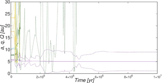
Perihelion distance q, semimajor axis a and aphelion distance Q of the five planets versus time according to our RA15 simulation with zero starting time for an unstable system in a D cluster. Note the very low perihelion distances reached by Saturn and – especially – by Jupiter after 2.3 and 2.5 Myr, respectively. For styles and colours of the curves, see the caption of Fig. 2.
The minimum perihelion distance of Saturn is 0.077 au, and that of Jupiter is 0.013 au. Noting that the semimajor axes of hot Jupiters extend to nearly 0.1 au, both gas giants are thus candidates for becoming hot Jupiters by tidal circularization. This means that the embedded cluster environment indeed appears to provide a mechanism for the production of hot Jupiters. But our results at large show this to be a rare outcome. Thus, it cannot be expected to make a major contribution to the observed hot Jupiter population. We note that this is consistent with the finding by Winter et al. (2020) that hot Jupiter host stars are strongly concentrated to overdense regions in the phase space of the Galactic disc. Indeed, there is no reason for the fate of a star in its embedded cluster to correlate with its presence in such an overdense region up to ∼1 Gyr later.
Concerning our NAMD distributions, we emphasize that there is a well-defined limit between the largest values of stable systems and the smallest values of unstable systems (see Fig. 5). Checking this in detail, we find that the critical NAMD separating the two kinds of systems is given by the minimum eccentricities of Uranus and Neptune needed for the amount of orbital crossing to allow chaos to be induced by close encounters within the investigated time-scale. We note the very good agreement between our empirical result and the tentative estimate of the borderline between order and chaos of orbital evolutions provided by Turrini et al. (2022).2
For comparison with the NAMD distribution of observed exoplanets, the best available source is the recent paper by Turrini et al. (in preparation), where a homogeneous sample of planets with well characterized host stars is analysed. Considering that the NAMD is independent of the size of the planetary system, a comparison of the ranges of NAMD seems relevant although our systems are much larger than those so far observed. The agreement is good. The sample of Turrini et al. (in preparation) extends from 0.005 to 0.3, while our sample extends from 0.003 to 1.0. Here we have neglected our one-planet systems (M2 = 1), which are also discarded by Turrini et al. (in preparation). Only three of our systems stand out from the range of observed exoplanets, having NAMD ≈ 1.0, and two of these contain planets with inclinations of 90° or more.
Even though the good agreement seems encouraging, a few caveats have to be borne in mind. It is possible that the observed exoplanet systems, being of small size, have been destabilized by internal interactions rather than external ones, while leading to the same range of NAMD. The lack of the small NAMD values characterizing stable systems among the observed exoplanets also indicates that real planetary systems are more easily destabilized than we find by assuming the initial system to be large and inherently stable. Another issue relates to the possibility of unobserved, distant exoplanets in high-eccentricity orbits, causing an underestimate of the actual NAMD in the observed sample (Turrini et al., in preparation).
5 CONCLUSIONS
We have simulated the dynamical evolution of a planetary system with five members representing the likely precursors of our solar system according to the Nice Model (Nesvorný & Morbidelli 2012) as affected by the perturbing effects of a surrounding stellar cluster. For the latter we use simulations of embedded clusters spanning 10 Myr from inception. While our study focuses on one specific type of initial planetary system, we believe that our range of cluster environments yields a reasonable coverage of the environments facing the majority of solar-type stars in the Galaxy.
Our most important finding is a significant likelihood of dynamical chaos leading to breakdown of the system during the investigated time span, as induced by the cluster effects. This interpretation accounts for the likely cancellation of cluster effects as long as the natal gas disc remains and the likely distribution of disc lifetimes. We also find that, in the case of relatively short lifetime, the breakdown rate is particularly high in strongly concentrated clusters. This is explained by the fact that such clusters involve very high number densities in the central regions during the early phase of evolution.
In order to study the detailed mechanism for the onset of orbital chaos as well as the outcome in terms of end states, we have used a large sample of unstable systems resulting from simulations, where the gas disc is neglected and cluster effects act over the entire time period. Almost exclusively, we find that orbital chaos is triggered by one or more close encounters with cluster stars, and here the massive binaries stand out as very efficient agents. The initial effect is the excitation of eccentricities in the orbits of Uranus and Neptune, leading to orbital crossing and close encounters. This, in turn, easily spreads to the inner neighbour (the hypothetical ice giant referred to as Planet 5) and then further to Saturn and Jupiter.
As planetary end states, we have considered physical destruction by planet–planet or Sun–planet collision, dynamical ejection from the solar system, and survival involving extraction into orbits with semimajor axes exceeding 100 au. The fourth end state is the absence of all the above, meaning survival in orbits with smaller semimajor axes. Jupiter always belongs to the last category except a few cases of collisions. Ejections and extractions mostly concern the three outer planets. The final multiplicities of the systems tend to be high, if only destruction end ejection are counted as loss processes, but including also extractions, the multiplicities are mostly low.
The final values of the NAMD exhibit a very clear dependence on whether order or chaos dominates the orbital evolutions. The critical value separating the two regimes is about 2 × 10⁻³, i.e. 100 times the initial NAMD of the system, and it is essentially set by the likelihood of close encounters between Uranus and Neptune. Our unstable systems are found to fit well with observed exoplanet systems, while observed counterparts of our stable systems are very rare. We tentatively suggest that this may be due to a large importance of internally triggered instabilities in the observed, much smaller systems.
Our results on the likelihood of ejection or extraction also lead us to suggest consistency with the indicated abundance of low-mass, free-floating planets based on microlensing observations. Finally, we note that the orbital chaos leading to breakdown sometimes induces extremely small perihelion distances of Jupiter or Saturn – small enough to allow the possibility of evolution into hot Jupiters by tidal circularization. However, based on the rareness of this outcome, we conclude that observed hot Jupiters are only rarely formed due to environmental effects in embedded clusters.
ACKNOWLEDGEMENTS
Discussions on this and related topics within the Ariel WG on Planet Formation are gratefully acknowledged. We are indebted to an anonymous referee for advice that greatly improved the quality of this paper. The calculations were made at the Poznań Supercomputing and Networking Center.
DATA AVAILABILITY
Data available on request.
Footnotes
References to previous papers on this model are given in the quoted paper.
See fig. 11 of the quoted paper.
