


ABSTRACT
While observations of the stationary component of pulsar radio signals have in many ways formed the basis of our understanding of radio pulsars, the statistical deviations of these signals contain information that has become increasingly relevant. Using high time–frequency resolution data from the MeerKAT telescope, we study the self-noise of the autocorrelation function of six radio pulsars. The self-noise of the autocorrelation function is used to investigate the statistics of the observed radio signals on nanosecond time-scales and for five pulsars it is found to deviate from the expected form for a Gaussian process. Comparing the measured distribution of the intensity fluctuations of the on-pulse window to simulated models, we find that a mixture model comprising a Gaussian process and a Bernoulli-sampled Gaussian process is able to produce the excess self-noise while also producing the observed distribution of intensities. The parameters of the mixture model describing the signals are estimated for three of the pulsars in our sample group. Studies of the statistics presented in this work provide observational information for constraining the numerous theories of pulsar radio emission mechanisms. The mixture model suggested in this work would produce excess timing residuals for high signal-to-noise ratio observations when compared to that expected for a Gaussian process. Additionally, the measure of spectral self-noise provides a means of separating Gaussian and non-Gaussian processes that provides a potential basis for the development of alternative pulsar detection algorithms.
1 INTRODUCTION
Any discrete and wide-sense stationary signal can be expressed as the superposition of a deterministic component and an unpredictable random component (Wold 1938). In pulsar astronomy, the study of integrated profiles is the study of the pulsar’s stationary behaviour. This behaviour has formed much of the foundation of our understanding of the nature of pulsars. It is also instrumental to the scientific community, being the means by which pulsars are timed. However, emission models have become increasingly sophisticated as to explain the rich body of observational phenomena. Additionally, as observing instruments become ever more sensitive, it is the self-noise of pulsar signals that places the limit on pulsar timing precision (Liu et al. 2011; Osłowski et al. 2014; Shannon et al. 2014). An understanding of both the deterministic and the stochastic components of pulsar radio signals is required in order to fully characterize the process by which they are generated. Such understanding may also assist in developing improved methods for pulsar timing and more sensitive search algorithms for the detection of ever more distant pulsars. Single-pulse studies and investigations of the phase-resolved field statistics of pulsars have classically been faced with several challenges: storing and operating on the massive data quantities associated with raw voltages, the high performance requirements of the observing instrument, and also separating the effects of the emission mechanism from propagation effects. Technological innovation has at least addressed the first two of these issues to a large extent. In this work, we demonstrate the usefulness of the study of deviations from stationary behaviour; the random fluctuations of the short-time autocorrelation function are used for model comparison between various signal model hypotheses for the radio emissions of six pulsars.
When considering radio pulsar astronomy as a whole, it is worth appreciating the impact of integrated profiles. It was not long after the discovery of the first radio pulsar signals (Hewish et al. 1968; Pilkington et al. 1968) that rotating neutron stars were postulated as the source of the strange signals (Gold 1968; Pacini 1968). Though the model of rotating neutron stars has long since been accepted (Arons 1979), the emission mechanism itself remains elusive. Fundamental to theories of the emission process is the complex magnetosphere of the pulsar, which produces a radiating beam at open magnetic field lines near the magnetic poles (Goldreich & Julian 1969). In the early days of pulsar astronomy, an amplitude-modulated Gaussian noise process was often implicitly assumed to describe the observed signal (Rickett 1975) with the integrated pulse profile describing the cross-section of the radiating beam as it passes over the observer. For such a source-signal model one expects the observed electric field to be defined entirely by means and covariances and for pulse profile estimates to be consistent with a well-defined variance. Indeed, the integrated pulse profiles of radio pulsars have been found to be remarkably stable for integration over large numbers of pulses (Helfand, Manchester & Taylor 1975). This property forms the fundamental basis for pulsar timing; it can be assumed that a folded profile of a small number of pulses is equivalent to a stable template with a scaled amplitude, a time offset and with additive Gaussian noise introduced (Lorimer & Kramer 2004). The pulse time of arrival (TOA) is ordinarily estimated by correlating the short-time profile with the template profile in the Fourier domain (Taylor 1992). TOAs are then mapped to emission times at the pulsar and compared to simple timing models. Timing residuals are the differences between estimated emission times and model emission times (Edwards, Hobbs & Manchester 2006) and are intrinsically linked to the stability of short-time profiles. The observation of individual highly stable millisecond pulsars have allowed for unique tests of general relativity (van Straten et al. 2001; Kramer et al. 2006; Weisberg, Nice & Taylor 2010). Pulsar timing arrays that simultaneously observe the arrival times of several pulsars have been implemented with the intention of detecting gravitational waves (Hobbs & Dai 2017), relying specifically on a subset of highly stable pulsars (Verbiest et al. 2009). Aside from their importance in timing applications, the study of the various pulsar profiles and their morphology provides insight into the pulsar emission mechanisms and has led to the development of taxonomies such as the core and conal categorization by Rankin (1983).
For radio pulsars it is practical to assume a stationary linear process modulated by axial rotation as this is mathematically convenient and easily conceptualized. However, the vast body of observed phenomenology makes it increasingly difficult to explain pulsar radio radiation with such a model. The advent of coherent dedispersion revealed the existence of fine structures in integrated pulse profiles (Hankins 1971). Some pulsars spontaneously emit single pulses with quasi-periodic structures (Boriakoff, Ferguson & Slater 1981), which has recently also been observed in millisecond pulsars (De, Gupta & Sharma 2016; Liu et al. 2022). Single pulses are often found to be narrower than the integrated profile and may drift across the pulse phase (Drake & Craft 1968). These drifting subpulses have recently been found to possess unexpected polarization properties and phase–amplitude relationships (Wen et al. 2020; Primak et al. 2022). While these observations suggest more complicated magnetospheric processes than originally anticipated, perhaps stranger are the observations suggesting abrupt changes in the magnetosphere. Examples are the apparent mode-changing behaviour that impacts both pulse profile and spin-down rate in some pulsars (Lyne et al. 2010), and the pulse-to-pulse memory observed for the Vela pulsar (Palfreyman et al. 2011). The complex nature of pulsar radio signals manifests itself also in a practical sense, since the timing residuals of many pulsars deviate from forms predicted for thermal noise and simple random walk models of the profile parameters alone (Hobbs, Lyne & Kramer 2010). For some pulsars these deviations are correlated with the occurrence of high emission levels within specific phase regions (Vivekanand 2001; Osłowski et al. 2011). This suggests a short-time profile variability that is greater than anticipated and that occurs primarily within subregions of the pulse. The variability may be caused by intrinsic amplitude variations due to the occurrence of latent components or giant subpulses (Johnston et al. 2001; Chen et al. 2020), by non-Gaussian signal statistics or a combination thereof. An alternative signal model to amplitude-modulated Gaussian noise is amplitude-modulated shot noise, as proposed by Cordes (1976), possibly caused by emission events such as proposed ‘sparks’, a rapid breakdown of extreme potential differences caused by gaps in the magnetosphere (Ruderman & Sutherland 1975; Gil & Sendyk 2000).
The complexity and variety of the proposed emission models motivate the application of novel analysis methods using the departure of the single-pulse estimates from their stationary behaviour. Cairns, Johnston & Das (2001) demonstrated that the variability of the phase-resolved field intensity provides a powerful tool for constraining pulsar emission mechanisms, pointing out that improvements in astronomical instrumentation now allow for such studies. Jenet & Gil (2003) constructed a statistical test for constraining the emission mechanism by means of the intensity modulation index, though the application yielded inconclusive results both in the original sample group and also in a later study (Crawford et al. 2013). Yet another example of the application of variability statistics to pulsar radio signals is the modified coherency index, proposed by Jenet, Anderson & Prince (2001) as a means for detecting non-Gaussian pulse components and estimating their characteristic widths. However, Smits et al. (2003) have pointed out that the results of this statistical test are due to scintillation effects and not the intrinsic variability of the pulsar radio emissions themselves. Beyond constraining emission models, the study of emission variability offers a powerful means for diagnosing timing residuals. As the signal-to-noise ratio (SNR) of pulsar observations approaches unity, it is the self-noise of the desired signal and not the instrumental noise floor that limits the precision of pulsar timing. It has been proposed that characterizing and accounting for single-pulse variability may significantly reduce the residuals in pulsar timing (Kerr 2015).
In this work, we analyse the self-noise of the autocorrelation function as originally proposed by Gwinn & Johnson (2011). The analysis is applied to observations of six radio pulsars. The pulsars were observed using the MeerKAT telescope and the sample group includes both normal and millisecond pulsars. The objective is to compare the achieved measurements with those expected for an amplitude-modulated Gaussian process, an amplitude-modulated shot noise process with a determined number of emission events and with a Bernoulli-sampled Gaussian process. None of the pulsars studied in this work have been previously analysed in this way. The expected result for the Gaussian model has previously been provided by Gwinn & Johnson (2011), as well as a discussion of the result for the shot noise model. In this work, we have applied geometric arguments to derive the expected result for the shot noise model and introduce an approximate form of the expected results in the case of the Bernoulli-sampled Gaussian process. The mathematical framework for the experiment is outlined in Section 2 and the observations are described in Section 3. The results are provided in Section 4 and discussed in Section 5, the conclusion of the work is given in Section 6.
2 MATHEMATICAL TOOLS
2.1 Assumptions and notation
In this work, the mathematical notation is kept consistent with that of Gwinn & Johnson (2011) where possible. The radio signal generated at the pulsar is modelled as a polarized, wideband, and circular complex Gaussian sequence, en. The individual samples of the sequence are uncorrelated and have a uniform variance of unity. The sequence is modulated by physical processes at the pulsar, most notably its axial rotation, transforming the stationary process into a non-stationary one when observed along a single line of sight. In practice, the largely periodic nature of the modulating process produces observations that are well suited to cyclostationary analysis (Demorest 2011); the individual samples of the modulated sequence remain uncorrelated but now display a time-dependent variance with a fundamental frequency determined by the pulsar’s rotational frequency.
2.2 The self-noise of various processes
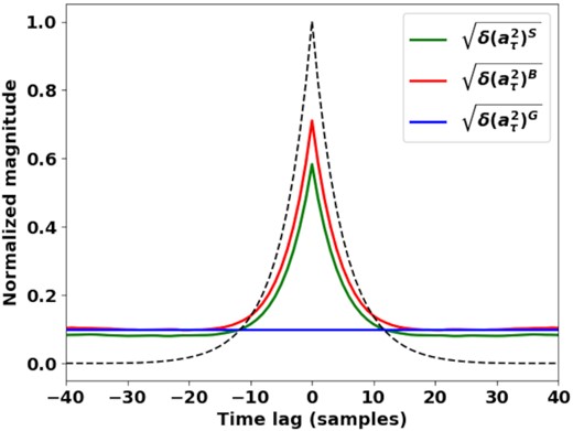
The noise of the autocorrelation function for the simulated outcomes of an exponential propagation response driven by various random processes. The dashed line is the average autocorrelation function of the channel. All functions have been normalized so that the zero-lag value of the signal is unity. A value for Nν of 256 is used and the propagation response time is five samples. ne of the shot-noise process is 3 and p of the Bernoulli-sampled Gaussian process is ne/Nν.
2.3 The effects of additive noise and amplitude variations
3 OBSERVATIONS AND DATA PROCESSING
The six pulsars were observed in 2020 November using the MeerKAT radio telescope. Each observation was approximately 300 s in duration. Only 52 of the 64 antennas were used in the observation as 12 antennas were undergoing maintenance at the time. The observations used the L-band receivers with a bandwidth of 856 MHz centred at 1284 MHz. Each receiver captured two linear orthogonal polarizations with an analogue-to-digital (ADC) sampling rate of 1712 MHz and a resolution of 10 bits. The telescope was used in tied-array mode. The data from each antenna were channelized into 1024 frequency channels and then coherently superimposed. Channelization was achieved using a 2048-channel polyphase filterbank. Half of the channels are redundant due to spectral symmetry and are discarded. The resulting data stream is a series of complex baseband signals, each with a bandwidth of 836 kHz, a sample period of 1.2 |$\mu$|s and 8-bit resolution for both real and imaginary components. Detailed information regarding the signal chain is presented by van der Byl et al. (2022). The data are recorded at the output of the beamformer, taking advantage of the high time–frequency resolution and sensitivity of MeerKAT, which has already proven itself as a powerful instrument for pulsar astronomy (Bailes et al. 2020) and pulsar detection (Wang et al. 2022). The data products of the pulsar timing user-supplied equipment (PTUSE) system are also recorded but are used only for data verification. Only data from the spectral channels spanning from 965 to 1145 MHz are used in this analysis, as this band is found to be particularly radio quiet during the observation.
Parameters of the observed pulsars, each of which was observed for approximately 300 s. The pulse frequencies are measured and the mixture model parameters are those estimated in this work. pNν is the average number of impulsive events per window. The normalized variance is the contribution of the Bernoulli-sampled Gaussian process to the total variance of the mixture process, given as a number between zero and one. The scattering time-scales are calculated for the lower end of our observing band, 965 MHz, using values found in the literature. The γ values are measured values where possible. Where no measured values were found the value of 4.4 is assumed, as denoted by an asterisk (*). The flux density is the average at 1400 MHz and is taken from the Australia Telescope National Facility (ATNF) Pulsar Catalogue (Manchester et al. 2005a) at https://www.atnf.csiro.au/research/pulsar/psrcat/.
| Pulsar | Pulse frequency | DM | τsc | γ | Flux density | Np | pNν | Normalized variance | Nν |
|---|---|---|---|---|---|---|---|---|---|
| (Hz) | (pc cm−3) | (|$\mu$|s) | (mJy) | ||||||
| J0437−4715 | 173.69 | 2.6 | 0.0042 | 4.4* | 150.2 | 45 000 | 1.4 | 0.78 | 432 |
| J0536−7543 | 0.8026 | 18.58 | 0.13 | 4.4* | 8.70 | 204 | 18.8 | – | 432 |
| J0742−2822 | 5.9964 | 73.73 | 16.9 | 3.8 | 26 | 1400 | 6.25 | 1 | 64 |
| J0835−4510 | 11.185 | 67.99 | 43.7 | 4.45 | 1050 | 2800 | 5.76 | 0.8 | 256 |
| J1644−4559 | 2.1973 | 478.8 | 12587.6 | 3.84 | 300 | 500 | 29.62 | – | 32 768 |
| J0737−3039A | 44.086 | 48.92 | 6.92 | 4.4* | 3.06 | 11 520 | – | – | 64 |
4 RESULTS
The analysis performed in this work is sensitive to changes in the propagation response and to amplitude variations both within and between the spectra used to form the signal. Each pulsar is unique and some of those analysed here are known to have exotic single-pulse behaviours that would impact the results if unaccounted for. We briefly detail the known behaviour of each pulsar and how the analysis was performed in each case. The results of the analysis for each pulsar are provided. We begin with the two pulsars for which the scintillation bandwidth is resolved by the filterbank and then proceed to the four for which subchannelization is required.
4.1 J0437−4715
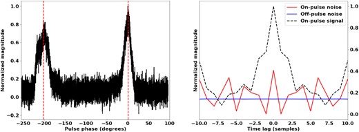
This pulsar is a very bright nearby millisecond pulsar discovered by Johnston et al. (1993), which has been the focus of many individual pulsar studies. The extreme stability of J0437−4715 has allowed for timing accurate enough to facilitate unique tests of general relativity (van Straten et al. 2001). A study of single pulses from this pulsar by Jenet et al. (1998) found that the emissions are similar in structure to those of regular pulsars, inferring a similar emission mechanism between regular pulsars and millisecond pulsars. Early estimates of the scintillation parameters of this pulsar were not in agreement and later studies found that the scintillation pattern of J0437−4715 is actually described on two scales and not one (Gwinn, Hirano & Boldyrev 2006; Smirnova, Gwinn & Shishov 2006). Fortunately, due to the proximity of the source, neither of these scintillation scales result in a scintillation bandwidth narrower than the spectral resolution of the filterbank applied in this study. In fact the scintillation bandwidth is well resolved by the filterbank and so the spectra are analysed without subchannelization.
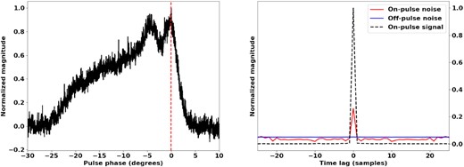
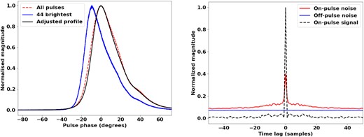
Fig. 2 shows the integrated pulse profile of the brightest pulses selected out of this observation compared to the total profile. The profile of the brightest pulses is significantly narrower than the total profile and the maxima of the two profiles are aligned – a known characteristic of this pulsar (Jenet et al. 1998). The on-pulse window for the analysis is chosen to lie on the peak of the integrated profile. The rate at which the filterbank produces spectral estimates is rapid enough that five consecutive spectra can be taken from the on-pulse window, over a phase region corresponding to only 5 per cent variation of the integrated profile. In this way, the number of sampled spectra is increased by treating five consecutive spectra from a narrow phase region of a single pulse as if they were sampled at a single phase on five separate pulses. After removal of pulses corrupted by RFI, about 200 000 independent spectra remain. The signal and the noise of the autocorrelation function are calculated for the off-pulse window and used to calculate the signal and noise for the pulsar from the on-pulse window. Both the signal and noise functions are normalized by the magnitude of the signal at zero lag, which enforces the normalization assumptions of Section 2.1. The result is illustrated in Fig. 2. The argument of the autocorrelation function – the lag τ – represents sample offsets in the original ADC voltage data, not to be confused with the samples of the filterbank output. The statistics of the observed signal are therefore estimated on the nanosecond time-scale.

The integrated profile of the brightest 1000 pulses of J0437−4715 overlaid on the total pulse profile, shown on the left. The vertical line indicates the position in pulse phase at which the spectra are sampled. The normalized on-pulse and off-pulse noise functions are shown on the right. The functions have been normalized such that the signal is unity at zero lag.
When analysing the forms of the measured noise functions the value of Nν is double the number of spectral channels in the spectra, as both polarizations are used in the estimates. The noise of the off-pulse window is a constant that is in agreement with that expected for a white Gaussian process. The on-pulse signal function is an impulse at zero lag. The on-pulse noise function is also an impulse at zero lag except with an added DC bias. The value of the on-pulse noise function decays for lags different to zero but there is no noticeable deficit for high lags and the value remains the same as that of the off-pulse window. Given the mathematical forms provided in Section 2.2 this result corresponds to a Bernoulli-sampled Gaussian process with an estimated pNν of 2.55, which corresponds to the average number of shot events per spectral accumulation.
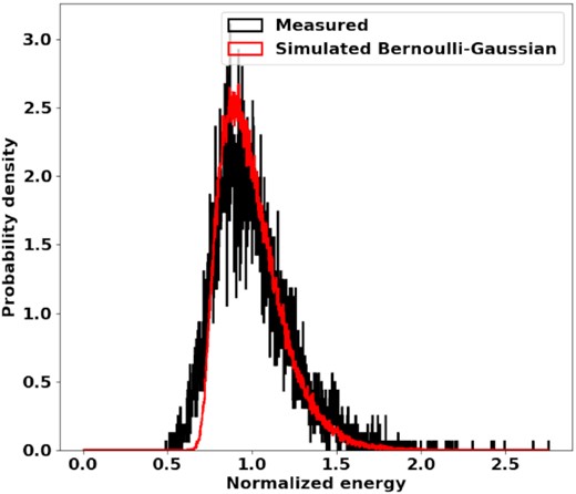
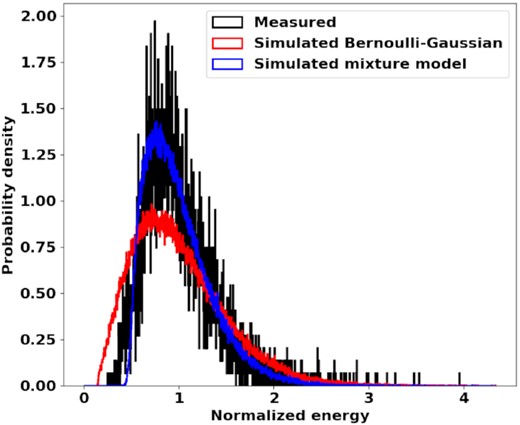
However, amplitude modulations of sufficient form may also cause exactly the noise function measured. In fact, Jenet et al. (1998) found that the intensity autocorrelation function and intensity modulation index for J0437−4715 are consistent with that expected for an amplitude-modulated Gaussian signal. On its own the noise function is not strong evidence of the signal hypothesis. For each spectrum, the spectral channels are squared and summed to measure the total energy, which corresponds to the zero-lag value of the autocorrelation function. The measured energies are binned and used to construct the histogram in Fig. 3. There is clearly significant variation in the energy estimates that are seen to take on a non-Gaussian distribution. This is not atypical of radio pulses from bright pulsars – for several examples, see Parthasarathy et al. (2021). If the underlying signal model were Bernoulli–Gaussian, though, then one would expect variations that take on a chi-squared distribution with a number of degrees of freedom constrained by pNν. We simulate a Bernoulli–Gaussian process with the estimated pNν value and add Gaussian noise to achieve the measured SNR. The simulated process is used to generate spectra for which the energy is calculated. The energies of the simulated and measured signal are binned and used to estimate the corresponding probability density functions, as shown in Fig. 4. The simulated distribution is similar to the measured distribution but is not peaked enough. In other words, while the Bernoulli–Gaussian process does produce the observed average estimation error of the zero-lag autocorrelation value, it does not produce the correct distribution of estimates. At the very least, the result demonstrates that the natural energy variations expected for a windowed Bernoulli–Gaussian signal are comparable to the measured variations of a windowed pulsar radio signal. In this way we relate the statistics of the signal on a nanosecond scale with the statistics of intensities accumulated over the microsecond scale.
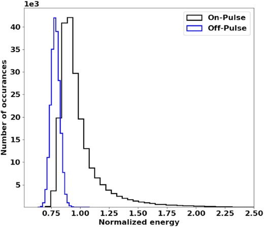
A histogram of the energies of spectra from the on-pulse and off-pulse sample groups for J0437−4715.
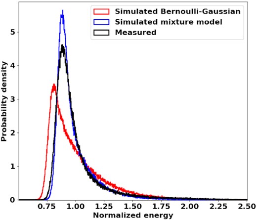
The estimated probability density function of the observed on-pulse spectral energies versus the density functions of outcomes from the simulated models for J0437−4715. The spectral energies have been normalized so that the mean energy of the measured on-pulse distribution is one.
The simulation would require a lower pNν value to achieve the steeper tail of the measured data. However, lowering pNν would also shorten the length of the tail and would produce a different noise function to that observed. We investigate the possibility of a mixture model, whereby the pulsar signal is modelled as a Bernoulli-sampled Gaussian process (representing large but infrequent impulses) superimposed onto a Gaussian background process. This is equivalent to a two-component Gaussian mixture model where both components have zero mean and the component with larger variance has a mixture weight equal to the Bernoulli probability p.
We constrain the variance of the mixture components and the pNν value such that the noise function is equivalent to that which is observed. Since the Bernoulli–Gaussian component is solely responsible for the excess noise at zero lag, decreasing the variance of the Bernoulli–Gaussian component requires a decrease in the pNν value in order to maintain the observed noise function. The resulting energy distribution has a sharper tail but largely maintains the tail length. The normalized variance of the Bernoulli–Gaussian component is its relative contribution to the total variance of the process, given as a number between zero and one. We achieve the best fit with a normalized variance of 0.78 for the Bernoulli–Gaussian component and a pNν value of 1.4. We point out that, since Nν includes the in-phase and quadrature spectral channels of both polarizations, pNν may be misleading in the case of a strongly polarized source. For cases where the observed polarization is parallel to one of the receiver polarizations, the value of pNν can be doubled without loss of correctness (as all of the shot events would need to occur within half of the spectra). The energy distribution of the mixture model is found to match the form of the measured data well, but overshoots the peak and underestimates the rise.
4.2 J0536−7543
This pulsar provides good contrast to J0437−4715, as it is an order of magnitude fainter and also has a pulse period greater than 1 s. While many of the other pulsars investigated in this work appear extensively in the literature and display a host of intriguing behaviours, J0536−7543 is largely unremarkable. While it is not known to glitch (Yu et al. 2013) J0536−7543 has been found to null in the 1308−1518 MHz band (Wang et al. 2020). We only capture 200 pulses for this pulsar and are therefore unable to construct a stable profile of the brightest pulses. We choose our on-pulse window to lie on the second peak and sample 220 consecutive spectra, again selecting a window that achieves minimal profile variation. After RFI removal we are left with approximately 40 000 spectra. We compute the on-pulse and off-pulse signal and noise in the same way as for J0437−4715. Again the off-pulse window produces the expected result and the on-pulse noise is a shifted impulse, as shown in Fig. 5. Despite being more than 10 times weaker than J0437−4715 and producing only a sixth of the spectral samples, the excess on-pulse noise is clear. In this case however, there is a noticeable deficit in the noise for non-zero lags, which suggests a determined number of shot noise events in each window. Again we would prefer to analyse the energy distribution to check that the excess noise is not due to pulse-to-pulse amplitude variations. However, the on-pulse energy distribution is barely distinguishable from that of the noise floor and thus we cannot confirm the model as we have done in the case of J0437−4715. In Table 1, we provide the estimated parameters for the pulsar assuming a Bernoulli-sampled Gaussian signal model.
The integrated profile of J0536−7543, shown on the left. The vertical line indicates the position in pulse phase at which the spectra are sampled. The normalized on-pulse and off-pulse noise functions are shown on the right. The functions have been normalized such that the signal is unity at zero lag.
4.3 J0742−2822
This pulsar was discovered during the Bologna 408-MHz Pulsar Search Project (Bonsignori-Facondi, Salter & Sutton 1973). It is a bright radio emitter that also emits gamma-rays. This pulsar is known to undergo emission state changes and spontaneously shift between multiple spin-down rates. It was one of the pulsars investigated in a long-term study on pulsars with this trait (Lyne et al. 2010). J0742−2822 is also known to intermittently switch between several profile shapes. Though other pulsars with multimodal spin-down rates were found to have a correlation between their pulse width and spin-down rate, the correlation between these parameters was not significant for J0742−2822. It was theorized that the correlation between the pulse width and spin-down rate became stronger after the occurrence of a glitch (Keith, Shannon & Johnston 2013). Long-term studies of this pulsar found that glitches do not increase the correlation between spin-down rate and pulse width. The pulsar has at least four modes of spin-down rate (Dang et al. 2021). The integrated pulse profile of the brightest pulses versus that of all pulses is illustrated in Fig. 6. While the profile of the brightest pulses is narrower than the total profile, it does not differ in an extreme manner as is the case for J0437−4715 and Vela.
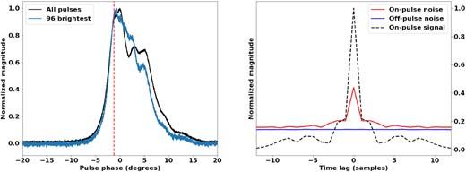
The integrated profile of the brightest 96 pulses of J0742−2822 overlaid on the total pulse profile, shown on the left. The vertical line indicates the position in pulse phase at which the spectra are sampled. The normalized on-pulse and off-pulse noise functions are shown on the right. The functions have been normalized such that the signal is unity at zero lag.
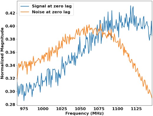
The spectra are sampled at the peak of the profile of the brightest pulses. This time the filterbank data cannot be used directly but must be subchannelized, as the scintillation bandwidth for this pulsar is smaller than the spectral resolution of the filterbank. Successive samples of the filterbank output are Fourier transformed to achieve this. For this pulsar we choose to subchannelize by a factor of 32 and discard three subchannels at the fringes of each spectral channel as they are suppressed by the filterbank response. We sample eight consecutive subchannelized spectra per pulse and after removing RFI pulses are left with 8752 spectra. The signal and noise analyses are applied as before but each spectral channel is analysed separately. Excess noise is found at zero lag for nearly all of the 216 spectral channels. The normalized zero-lag noise values are plotted against frequency in Fig. 7 along with the normalized spectral channel intensity measurements. The noise measurements have been normalized by their corresponding zero-lag signal values and the signal measurements have been scaled so that their mean over frequency is the same as the mean of the noise. Effectively what is illustrated is the variation in power versus the variation in self-noise over frequency. The noise at zero lag is an indication of the impulsiveness of the signal in the particular band, with higher values corresponding to greater impulsiveness and sparsity. The on-pulse noise peaks remain relatively constant over frequency, varying around the mean value of 0.33. The impulse in intensity in the vicinity of 1130 MHz is also present in the noise spectrum. From inspecting the on-pulse and off-pulse dynamic spectra it is found to be caused by narrow-band RFI. Despite the impact of the RFI on the spectral channel intensity the zero-lag noise value remains relatively unaffected. The spectral channel at 1058 MHz is chosen to inspect the distribution of single-pulse energies. For this pulsar it is found that the estimated Bernoulli-sampled Gaussian process with a pNν of 6.25 is able to explain the observed distribution of energy estimates better than the constrained mixture model used for J0437−4715. This is shown in Fig. 8. The simulated model deviates from the measured distribution as an underestimation of the rise and an overshoot of the peak.
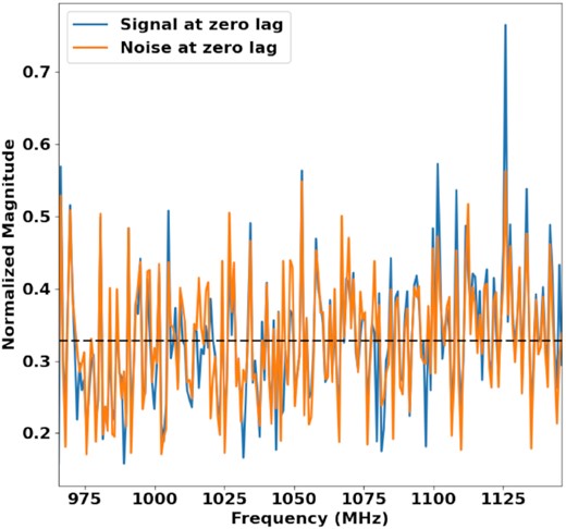
The frequency dependence of the zero-lag noise versus the zero-lag signal for J0742−2822. The dashed black line indicates the mean. The signal impulse in the vicinity of 1130 MHz is caused by narrow-band RFI.
The estimated probability density function of the observed on-pulse spectral energies versus the density function of outcomes from the simulated model for J0742−2822. The spectral energies have been normalized so that the mean energy of the measured on-pulse distribution is one. The spectral energies are from the 1058-MHz spectral channel.
4.4 J0835−4510
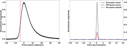
The Vela pulsar is a young, bright, and nearby pulsar that was discovered in one of the earliest pulsar surveys (Large, Vaughan & Mills 1968). This particular object has played a key role in understanding the nature of pulsars; its proximity to the Vela supernova remnant was a clue in determining the origin of the ‘pulsating radio signals’ before the rotating neutron star model had been commonly accepted. Additionally, it was the study of the polarization properties of the Vela pulsar that supported the development of the rotating vector model of pulsar radio polarization (Radhakrishnan & Cooke 1969) and early high time-resolution studies of Vela’s single pulse emissions were the first to employ coherent dedispersion (Hankins 1971). The proximity and brightness of Vela have made it the target of numerous single-pulse studies. While it has not been found to emit giant pulses, Vela is known to emit giant subpulses (Johnston et al. 2001; Chen et al. 2020). It is known that the brightest pulses are narrower on average than the average profile and arrive early. In fact, Vela’s pulse profile is a function of pulse strength, which could be due to independent pulse components that are active at different times and are emitted at different altitudes in the magnetosphere (Krishnamohan & Downs 1983). While Vela is not the only radio pulsar possessing an intensity-dependent pulse shape (McKinnon & Hankins 1993; Jenet et al. 1998), it is the only pulsar in our sample group known to have a single-pulse arrival time that is correlated with the pulse magnitude. The Vela pulses are so bright that the high-sensitivity data from MeerKAT allow us to estimate the pulse arrival time simply by measuring the maximum value of each pulse window. The deviation of the single-pulse maxima from the average value is plotted against the square root SNR value of each pulse. The result is shown in Fig. 9 and suggests a linear dependence between pulse intensity and arrival time, not a multimodal distribution. This result is consistent with a recent observation of drifting subpulses from Vela at high frequencies (Wen et al. 2020). Each Vela pulse in this analysis is shifted in time according to the best-fitting line, which decorrelates the pulse arrival time from its SNR and minimizes jitter. The pulse profile of the shifted pulses is noticeably narrower than the profile constructed without the correction, as shown in Fig. 10. Vela has been found to emit an increased number of bright pulses and a wider than usual pulse profile after the occurrence of a glitch (Palfreyman et al. 2016). While it is possible that this is due to an increase in the average pulse width, it is also possible that the wider pulse profile is due to a larger number of misaligned pulses. This may be due to increased activity of the emitting mechanism responsible for the leading component. This can be tested by correcting for pulse alignment after the occurrence of a glitch event, in the manner demonstrated here.
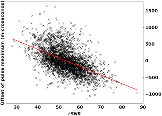
The deviation of each single pulse from the average arrival time plotted against root SNR for J0835−4510. The red line is the best-fitting one.
The integrated profile of the brightest 44 pulses of J0835−4510 overlaid on the total pulse profile, shown on the left. The spectra are sampled at zero pulse phase. The normalized on-pulse and off-pulse noise functions of J0835−4510 at 939 MHz are shown on the right. The functions have been normalized such that the on-pulse signal is unity at zero lag.
The propagation effects that act on the Vela pulsar radio signals are also novel. This is believed to be due to the Vela pulsar’s proximity to the Vela supernova remnant. The scintillation effects suggest that scattering occurs much nearer to the origin of the emissions than to the observer (Desai et al. 1992), which violates the usual assumption of the scattering screen being located mid-way between the observer and the source. The diffractive scintillation bandwidth of Vela for the band used in this work is much narrower than for other similar pulsars (Backer 1974). The dispersion measure is also known to change significantly over time (Petroff et al. 2013). We draw samples for the analysis from the peak of the corrected profile and subchannelize by a factor of 128 and discard 14 spectral channels on each end. From each pulse we draw two consecutive spectra and after the removal of RFI we are left with 5094 spectra. The analysis is performed in the same manner as for J0742−2822. We observe the zero-lag noise level as a function of frequency, compared to the normalized intensity, as shown in Fig. 11. The variance of the estimates is much smaller for Vela than for J0742−2822 but a significant variation in the mean is seen over frequency, which implies a change in the impulsiveness of the signal over the band. It is possible that using more samples to reduce the variance of the estimates for J0742−2822 may also reveal frequency-dependent variation. We choose the 939-MHz spectral channel for signal and noise analysis. As is the case for J0437−4715, a Bernoulli–Gaussian mixture model achieves a closer fit for the pulse-to-pulse energy distribution than a pure Bernoulli–Gaussian process. This result is illustrated in Fig. 12. The inferred pNν value for the Bernoulli–Gaussian process is 8.65 and the best-fitting parameters of the mixture model are a normalized variance of 0.8 with a pNν value of 5.76.
The frequency dependence of the zero-lag noise for J0835−4510 versus the zero-lag signal.
The estimated probability density function of the observed on-pulse spectral energies versus the density functions of outcomes from the simulated models for J0835−4510 at 939 MHz. The spectral energies have been normalized so that the mean energy of the measured on-pulse distribution is one.
4.5 J1644−4559
We find little mention of this pulsar in the literature. It is the most distant pulsar analysed in this work and its emissions are severely scattered. Despite these traits J1644−4559 is the third brightest pulsar in our sample group. There are 500 pulses from this pulsar in our observation of which all are detected. In order to resolve the scintillation bandwidth in this case, while meeting the Nyquist criterion in the frequency domain, the filterbank channels are to be subchannelized by a factor of 32 768 (going by the nearest radix-2 number). Practical limitations restrict us to a factor of 16 384. Our measurement is taken at 1040 MHz and the spectra are sampled mid-way on the rising edge of the pulse. Only one spectrum is sampled per pulse and the accumulation window includes the pulse peak. There is a significant zero-lag component in the off-pulse noise function, as shown in Fig. 13, but due to the limited number of pulses and the extreme subchannelization we are unable to fit a mixture model. Gwinn & Johnson (2011) have mentioned that measurements deviate from expected forms in cases where the spectral accumulation time is comparable to the propagation response time. We leave a detailed study of the on-pulse noise function of this pulsar for future studies. The estimated parameter values for our observation of J1644−4559 assuming a Bernoulli-sampled Gaussian process are listed in Table 1.
The integrated profile of J1644−4559, shown on the left. The vertical line indicates the position in pulse phase at which the spectra are sampled. The normalized on-pulse and off-pulse noise functions are shown on the right, as measured at 1040 MHz. The functions have been normalized such that the signal is unity at zero lag.
4.6 J0737−3039A
This pulsar belongs to the only known double-pulsar binary system and has an incredibly tight orbit of approximately 2.4 h. Its discovery has been pivotal in constraining the estimated rate of binary mergers due to its rapid orbital decay (Burgay et al. 2003). Pulse arrival timing of pulses from the double-pulsar system has provided an unparalleled tool for testing general relativity (Kramer et al. 2006). The companion of J0737−3039A, J0737−3039B, was not discovered in the original observation, as pulses from this object were only visible during narrow windows of the orbital cycle at that time. It was only in a follow-up observation that the much slower pulses of the companion were detected (Lyne et al. 2004). Soon after the discovery of the companion it was noticed that the window in which the companion was detectable was shrinking. Changes in the profile suggested that the beam had moved off our line of sight as a result of precession (Burgay et al. 2005). The companion object ceased to be detectable in 2008 March. Long-term observations of J0737−3039A show that the profile is relatively stable despite the precession of its companion. The profile of this pulsar is a double pulse that has strong linear polarization at the extreme leading and trailing edges (Manchester et al. 2005b). The orbit of this system is rapid enough that modulation is observed in the scintillation pattern of the dynamic spectrum (Ransom et al. 2004; Rickett et al. 2014) and eclipsing of J0737−3039A by its companion produces periodic breaks in the scintillation pattern. The effects of the Doppler shift on the observed spin frequency change rapidly enough to impact single pulse studies in a 5-min observation. We therefore update the pulse period and expected pulse position throughout the analysis to correct for the variable Doppler shift. The pulses from this pulsar are too faint for single-pulse detection and we are therefore unable to construct a profile from the strongest pulses. We sample two consecutive spectra from each pulse and after RFI removal approximately 16 000 spectra remain. The on-pulse and off-pulse signal and noise are calculated as previously described and are shown in Fig. 14. In the case of this pulsar there is no significant noise on the zero lag and the variance of the noise function is found to be more pronounced than for the other pulsars. We analyse both the leading and trailing edges at multiple frequencies but find nothing of significance.
The integrated profile of J0737−3039A, shown on the left. The vertical lines indicate the positions in pulse phase at which the spectra are sampled. The normalized on-pulse and off-pulse noise functions at 1146 MHz are shown on the right. The functions have been normalized such that the signal is unity at zero lag.
5 DISCUSSION
Gwinn & Johnson (2011) demonstrate how intermittency increases the estimation error of the second-order statistics of the process. Various processes can be modelled as distinct modulating functions applied to a stationary Gaussian process, and the self-noise of the autocorrelation function provides a means of discriminating between the processes. The modulating function is either pre-determined or is stochastic with the constraint that its net energy does not change between outcomes. The former case corresponds to a non-stationary Gaussian process whereas the latter represents a stationary non-Gaussian process. In this work, we consider a modulating function, fn, that only satisfies a constraint on its average energy. The approximate form that we present in equation (16) allows for pNν values less than one and can therefore be applied to highly sparse processes. We demonstrate explicitly that the noise deficit at high lags, previously predicted for the shot noise model by Gwinn & Johnson (2011), is not present in our model for a Bernoulli-sampled process. To the authors’ knowledge, this result has not previously been reported in the literature. In the case of pulsar radio signals, the Bernoulli-sampled process seems to be more intuitively satisfying than the shot noise model, which seems overly restrictive when considering the natural process observed.
The results yield noise functions that deviate from the expected form for a Gaussian process for all but one pulsar. It was proposed by Gwinn & Johnson (2011) that a shot-noise process with a determined number of shot events might cause a deficit in the noise function beyond lags within the filter response. We find a significant deficit in the noise function only for J0536−7543, which is the slowest rotating pulsar in our sample group. Our measurements also suggest that the impulsive events are unresolved in time by the ADC samples, as the autocorrelation noise function is the same width as the average autocorrelation function. We propose a Bernoulli–Gaussian and Gaussian mixture model as being responsible for the excess noise at low lags. We have sampled the spectra such that average amplitude variations within the sample windows are minimal. However, the noise forms may be caused by a Gaussian process with relative amplitude variations between the spectra. Through simulations we show that the proposed mixture models result in simulated interpulse amplitude variations that fit the observed data well. This does not definitively support either our proposed model or amplitude-modulated Gaussian statistics; rather, the results suggest that amplitude-modulated Gaussian statistics are not unique in producing the distribution of intensities at a narrow phase. Measurements of the moments of this distribution, such as the phase-resolved intensity modulation index, are therefore unable to discriminate between the various models that might produce the distribution. The result also demonstrates a unified theory for intensity fluctuations on time-scales on different orders of magnitude in pulsar radio signals. The extreme sparsity of the signal on nanosecond scales can cause significant variability of intensity estimates accumulated over microsecond time-scales. The estimated parameters for each pulsar assuming the proposed mixture model are presented in Table 1.
While the simulations do produce outcomes that closely resemble the observed data, there are mismatches. Most notably, the models tend to underestimate the number of outcomes on the rise and overestimate the number of outcomes at the peak. We also see that in many cases the average autocorrelation shows a diminished filter response. While the rate of change of the propagation response is approximately on the scale of the observation time in this work, the propagation response does undergo some change in our observations. Notably, the Vela pulsar displays exotic scintillation behaviour and the rate of change of the response due to diffractive scintillation is on the scale of 5 s in our band. Dealing with this issue in future studies can be achieved by incorporating the work found in Johnson & Gwinn (2012). It may also be useful to achieve the estimates by sequential two-point estimation of the signal and noise as a function of the signal as demonstrated by Gwinn et al. (2011). We also note that the work done here has not accounted for the effects of polarization and Faraday rotation. By enhancing the base model to include these effects it may be possible to account for the mismatch currently seen between the simulated models and the observations.
Lastly, the approach to estimation of the relevant statistics as performed in this work suffers from at least two major challenges. The requirement to accumulate windows on the time-scale of the propagation response produces an unwieldy amount of data and computational cost in the case of distant pulsars such as J1644−4559. Additionally, the stability of the estimate of self-noise as performed here necessarily requires a stable estimate of the signal. For weak pulsars such J0737−3039A, short observations do not provide high-quality estimates of the average autocorrelation function. The requirement for high-quality averages in the case of distant and slow pulsars, while also requiring the propagation response to be stationary, presents a unique signal processing challenge. The problem is compounded by the nature of radio pulsars themselves for which the statistics of interest are periodic outcomes, possibly containing features down to the nanosecond scale.
6 CONCLUSION
This work has demonstrated the usefulness of statistical deviations as a tool for radio pulsar science. The analysis of the self-noise of the autocorrelation function has been applied to radio signals from six pulsars. The results show a deviation from Gaussian statistics in all but one pulsar and only one pulsar is found to produce a significant noise deficit for lags beyond the filter response. While pulse-to-pulse amplitude variations of a Gaussian process might also cause such results, we show through simulations that Bernoulli-sampled Gaussian statistics on the nanosecond time-scale are able to explain fluctuations between intensity estimates accumulated on the microsecond time-scale, between pulses. These results do not offer conclusive evidence to support that the simulated processes are indeed those present in the signals analysed. However, we argue that the distribution of the phase-resolved intensity, and therefore its moments, is not unique to amplitude-modulated Gaussian statistics. The direct approach to estimating the noise statistics, as used in this work, is found to be sensitive to a changing propagation response, estimation errors of the signal, and is challenged by long propagation responses. More sophisticated estimation methods are required for future work. Determining the model for pulsar radio signals on short time-scales would offer valuable information for constraining the radio emission mechanism of radio pulsars, improving pulsar timing precision and detecting ever more distant radio pulsars.
ACKNOWLEDGEMENTS
The authors acknowledge the MeerKAT team for providing the raw data used in this work. The MeerKAT telescope is operated by the South African Radio Astronomy Observatory, which is a facility of the National Research Foundation, an agency of the Department of Science and Innovation, South Africa. The authors also acknowledge the reviewer for constructive feedback that has improved the quality of the paper.
DATA AVAILABILITY
The data underlying this paper will be shared on reasonable request to the corresponding author.
