


ABSTRACT
This paper continues our study of radio pulsar emission-beam configurations with the primary intent of extending study to the lowest possible frequencies. Here, we focus on a group of 133 more recently discovered pulsars, most of which were included in the (100–200 MHz) LOFAR High-Band Survey, observed with Arecibo at 1.4 GHz and 327 MHz, and some observed at decametre wavelengths. Our analysis framework is the core/double-cone beam model, and we took opportunity to apply it as widely as possible, both conceptually and quantitatively, while highlighting situations where modelling is difficult, or where its premises may be violated. In the great majority of pulsars, beam forms consistent with the core/double-cone model were identified. Moreover, we found that each pulsar’s beam structure remained largely constant over the frequency range available; where profile variations were observed, they were attributable to different component spectra and in some instances to varying conal beam sizes. As an Arecibo population, many or most of the objects tend to fall in the Galactic anticenter region and/or at high Galactic latitudes, so overall it includes a number of nearer, older pulsars. We found a number of interesting or unusual characteristics in some of the pulsars that would benefit from additional study. The scattering levels encountered for this group are low to moderate, apart from a few pulsars lying in directions more towards the inner Galaxy.
1 INTRODUCTION
The narrow emission beams of radio pulsars provide particular challenges because each shines towards the Earth only owing to a pulsar’s accidental alignment. Therefore, there is typically no direct means of discerning just what portion of the entire beam our sightline encounters. Multiple efforts to understand pulsar beamforms began shortly after the discovery of pulsars, and this history is reviewed in recent publications by both Olszanski et al. (2022) and Rankin et al. (2022). None the less, a comprehensive understanding of pulsar beamforms has remained elusive, but crucial to comprehending the physical mechanisms of pulsar dynamics and emission.
In what follows, we provide analyses intended to assess the efficacy of the core/double-cone beam model at frequencies down to the 100-MHz band, largely completing our efforts to study the population of Arecibo pulsars (declinations between about –1° and 38°) surveyed using the LOFAR telescope’s High Band by Bilous et al. (2016). Groups of Arecibo ‘B’ pulsars were analysed in Olszanski et al. (2022, Paper I) and Rankin et al. (2022, Paper II) using 1.4-GHz and 327-MHz observations, and this work similarly treats a remaining population of more recently discovered ‘J’ objects. Our overarching goal in these works is to identify the physical implications of pulsar beamform variations with radio frequency.
The Pushchino Radio Astronomy Observatory (PRAO) has long pioneered 103/111-MHz studies of pulsar emission using their Large Phased Array (LPA). Surveys by Kuz’min & Losovskii (1999, hereafter KL99) and Malov & Malofeev (2010, MM10) have provided a foundation for our overall work. More recently, the Low Frequency Array (LOFAR) in the Netherlands has produced an abundance of high-quality profiles with their High Band Survey (hereafter BKK+, PHS+ Bilous et al. 2016; Pilia et al. 2016) in the 100–200 MHz band as well as others in their low band (Kondratiev et al. 2016; Bilous et al. 2020; Bondonneau et al. 2019). In addition, decametric observations are available from the Kharkiv Array (Zakharenko et al. 2013; Kravtsov et al. 2022) as well as from the Long Wavelength Array (Kumar et al., in preparation).
A radio pulsar emission-beam model with a central ‘core’ pencil beam and two concentric conal beams has proven useful and largely successful both qualitatively and quantitatively in efforts to model the beam geometry at frequencies around 1 GHz (Rankin 1993b) and its appendix (Rankin 1993a, together hereafter ET VI; see Section 3). Few attempts, however, have been made to explore the systematics of pulsar beam geometry over the entire radio spectrum.1 Here, we present analyses aimed at elucidating the multiband beam geometry of a brighter group of ‘J’ pulsars within the Arecibo sky, most of which with observations down to the 100-MHz band.
In this work, Section 2 describes the Arecibo observations, Section 3 reviews the geometry and theory of core and conal beams, Section 4 describes how our beaming models are computed and displayed, Section 5 discusses scattering and its effects at low frequencies, Section 6 the overall analysis and conclusions, and Section 7 gives a short summary. The main text of the paper reviews our analysis while the tables, model plots, and notes are given in the Appendix. In this Appendix, we discuss the interpretation and beam geometry of each pulsar, and Figs A1–A21 show the results of analyses clarifying the beam configurations. Figs A22–A65 then give the beam-model plots (Fig. 1 provides an example) and (mostly) Arecibo profiles on which they are based. The supplementary material provides the Appendix and ascii versions of the three tables.
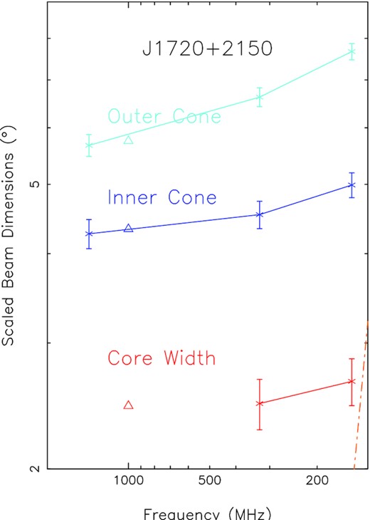
Sample core/double-cone beam model display for pulsar J1720+2150 (see Fig. A40). Curves for the scaled outer and inner conal radii and core width are shown – the former by |$\sqrt{P}$| and the latter by |$\sqrt{P}\sin \alpha$|. Conal error bars reflect the rms of 10 per cent uncertainties in both the profile widths and PPA rate (see the text), and the core errors also reflect a 10 per cent error. Further, J1720+2150 is a case where no scattering time has been measured and published, so an average value (Kuz’min 2001) is used – and the 10x average orange (dot–dashed) line is just visible at the lower right. The plots are logarithmic on both axes and labels are shown only for orders of 1, 2, and 5.
2 OBSERVATIONS
We present observations carried out using the upgraded Arecibo Telescope in Puerto Rico with its Gregorian feed system, 327-MHz (‘P-band’) or 1100–1700-MHz (‘L-band’) receivers, and either the Wideband Arecibo Pulsar Processors (WAPPs) or Mock spectrometer backends. At P-band four 12.5-MHz bands were used across the 50 MHz available. Four nominally 100-MHz bands centred at 1170, 1420, 1520, and 1620 MHz were used at L band, and the lower three were usually free enough of radio frequency interference (RFI) such that they could be added together to give about 300-MHz bandwidth nominally at 1400 MHz. The four Stokes parameters were calibrated from the auto- and cross-voltage correlations computed by the spectrometers, corrected for interstellar Faraday rotation, various instrumental polarization effects, and dispersion. The resolutions of the observations are usually about a milliperiod as indicated by the sample numbers in Table A1. For the lower frequency observations, please consult the paper of origin as referenced in this table. Where our Arecibo observations were poor or missing we made use of other published compendia (Barr et al. 2013; Foster et al. 1995; Han et al. 2009; Johnston & Kerr 2018; McEwen et al. 2020; Seiradakis et al. 1995; Weltevrede et al. 2007) and other studies (Brinkman et al. 2018; Janssen et al. 2009; Lorimer et al. 2006).
The observations and geometrical models of the pulsars are presented in the tables and figures of the Appendix. Table A1 describes each pulsar’s period, dispersion measure (DM), and rotation measure (RM), and then gives the sources for the observations and measurements at each frequency (see the sample below in Table 1). Table A2 gives the physical parameters of each pulsar, its period and spindown rate, energy loss rate, spindown age, surface magnetic field, the acceleration parameter B12/P2 and the reciprocal of Beskin, Gurevich & Istomin (1993)’s Q parameter (1/Q = |$0.5\ \dot{P}_{-15}^{0.4} P^{-1.1}$|) as in Papers I and II. The Gaussian fits use Michael Kramer’s bfit code (Kramer et al. 1994; Kramer 1994). The geometrical models are given in Table A3 as will be described below. Plots then follow showing the behavior of the geometrical model over the frequency interval for which observations are available, as well as Arecibo polarized average profiles where available.
Sample: Observation Information (see Table A1).
| Pulsar | P | DM | RM | MJD | Npulses | Bins | MJD | Npulses | Bins | References |
|---|---|---|---|---|---|---|---|---|---|---|
| (s) | (pc cm−3) | (rad m2) | ||||||||
| (L band) | (P band) | (≲100 MHz) | ||||||||
| J0006+1834 | 0.69 | 11.4 | –20.9 | 58887 | 3009 | 512 | 57844 | 1036 | 1024 | BKK + |
| J0030+0451 | 0.0049 | 4.3 | + 1.2 | Spiewak et al. (2022) | – | – | – | KTSD, 35 | ||
| J0051+0423 | 0.35 | 13.9 | –6.3 | 58887 | 16743 | 1108 | 58902 | 14844 | 1182 | PHS + ; ZVKU |
| J0122+1416 | 1.39 | 17.7 | –15 | 58972 | 1665 | 256 | 58950 | 2586 | 1036 | |
| J0137+1654 | 0.41 | 26.6 | –15.7 | 58886 | 16743 | 1024 | 58902 | 2886 | 1020 | BKK + |
| J0139+3336 | 1.25 | 21.2 | –42 | 58965 | 1185 | 1031 | 58951 | 1436 | 1040 | |
| J0152+0948 | 2.75 | 21.9 | –0.2 | 58299 | 1025 | 1056 | 57844 | 325 | 1024 | BKK + |
| J0245+1433 | 2.13 | 29.5 | – | – | – | – | 57844 | 1028 | 1013 | PRAO |
| J0329+1654 | 0.89 | 42.1 | + 5.8 | 56932 | 1028 | 1116 | 57123 | 1116 | 1049 | BKK + |
| J0337+1715 | 0.0027 | 21.3 | + 29.0 | 56760 | 365928 | 256 | 56584 | 365914 | 256 | |
3 CORE AND CONAL BEAMS
A full recent discussion of the core/double-cone beam model and its use in computing geometric beam models is given in Rankin (2022).
Canonical pulsar average profiles are observed to have up to five components (Rankin 1983), leading to the conception of the core/double-cone beam model (Backer 1976). Pulsar profiles then divide into two families depending on whether core or conal emission is dominant at about 1 GHz. Core single St profiles consist of an isolated core component, often flanked by a pair of outriding conal components at high frequency, triple T profiles show a core and conal component pair over a wide band, or five-component M profiles have a central core component flanked by both an inner and outer pair of conal components.
By contrast, conal profiles can be single Sd or double D when a single cone is involved, or triple cT or quadruple cQ when the sightline encounters both conal beams. Outer cones tend to have an increasing radius with wavelength, while inner cones tend to show little spectral variation. Periodic modulation often associated with subpulse ‘drift’ is a usual property of conal emission and assists in defining a pulsar’s beam configuration (e.g. Rankin 1986).
Profile classes tend to evolve with frequency in characteristic ways: St profiles often show conal outriders at high frequency, whereas Sd profiles often broaden and bifurcate at low frequency. T profiles tend to show their three components over a broad band, but their relative intensities can change greatly. M profiles usually show their five components most clearly at metre wavelengths, while at high frequency they become conflated into a ‘boxy’ form, and at low frequency they become triple because the inner cone often weakens relative to the outer one.
Application of spherical geometry to the measured profile dimensions provides a means of computing the angular beam dimensions – resulting in a quantitative emission-beam model for a given pulsar. Two key angles describing the geometry are the magnetic colatitude (angle between the rotation and magnetic axes) α and the sightline-circle radius (the angle between the rotation axis and the observer’s sightline) ζ, where the sightline impact angle β = ζ − α.2 The three beams are found to have particular angular dimensions at 1 GHz in terms of a pulsar’s polar cap angular diameter, ΔPC = 2.45°P−1/2 (ET IV Rankin 1990). The outside half-power radii of the inner and outer cones, ρi and ρo are 4.33°P−1/2 and 5.75°P−1/2 (ET VIb).
The outflowing plasma responsible for a pulsar’s emission is partly or fully generated by a polar ‘gap’ (Ruderman & Sutherland 1975), just above the stellar surface. Timokhin & Harding (2015) find that this plasma is generated in one of two pair-formation-front (PFF) configurations: for the younger, energetic part of the pulsar population, pairs are created at some 100 m above the polar cap in a central, uniform (1D) gap potential – thus a 2D PFF, but for older pulsars the PFF has a lower, annular shape extending up along the polar fluxtube, thus having a 3D cup shape.
An approximate boundary between the two PFF geometries is plotted on the P–|$\dot{P}$| diagram of Fig. 3, so that the more energetic pulsars are to the top left and those less so at the bottom right. Its dependence is |$\dot{P}=3.95\times \, 10^{-15}P^{11/4}$|. Pulsars with dominant core emission tend to lie to the upper left of the boundary, while the conal population falls to the lower right. In the parlance of ET VI, the division corresponds to an acceleration potential parameter B12/P2 of about 2.5, which in turn represents an energy loss |$\dot{E}$| of 1032.5 erg s−1. This delineation also squares well with Weltevrede & Johnston (2008)’s observation that high energy pulsars have distinct properties and Basu et al. (2016)’s demonstration that conal drifting occurs only for pulsars with |$\dot{E}$| less than about 1032 erg s−1. As previously mentioned, a sample of physical parameters is given in Table 2 and in full in Table A2.
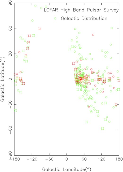
Plot showing the distribution of the LOFAR High Band Survey pulsar population (164; circles) on the sky in Galactic coordinates, and others (112; rectangles) studied here down to the –1.5° Arecibo southern declination limit. Pulsars with |$\dot{E}$| greater or less than 1032.5 erg s−1 are shown with red or green symbols, respectively. Clearly the core-emission dominated energetic objects lie both closer to the Galactic plane and Galactic Centre than their less energetic conal cousins.
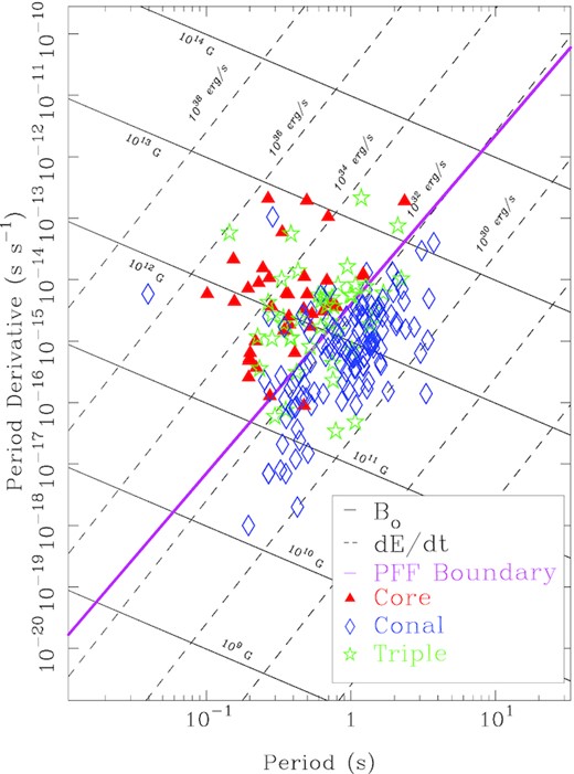
P–|$\dot{P}$| diagram showing the distribution of the LOFAR High-Band Survey pulsar population (194) – augmented by Arecibo pulsars studied here and in Papers I and II (110) – in relation to the PFF boundary. Core-emission-dominated pulsars tend to lie to the upper left of the Timokhin & Harding (2015) boundary line, whereas those with mainly conal emission fall to the lower right (see the text). Pulsars with core-cone triple T are distributed across both regions. This population has a smaller proportion of energetic core-dominated pulsars (32 per cent) than seen in the sky overall. Of particular interest are the two energetic pulsars that seem to be conal emitters, J0631+1036 and B1951+32.
Sample: pulsar parameters (see Table A2).
| Pulsar | P | |$\dot{P}$| | |$\dot{E}$| | τ | Bsurf | B12/P2 | 1/Q |
|---|---|---|---|---|---|---|---|
| (B1950) | (s) | (10−15 | (1032 | (Myr) | (1012 | ||
| s s−1) | erg s−1) | G) | |||||
| J0006+1834 | 0.694 | 2.10 | 2.479 | 5.2 | 1.22 | 2.5 | 1.0 |
| J0030+0451 | 0.0049 | 1e−5 | 35.0 | 7580.0 | 2.3e−4 | 9.5 | 1.8 |
| J0051+0423 | 0.355 | 2e−3 | 0.062 | 803.0 | 0.05 | 0.4 | 0.1 |
| J0122+1416 | 1.389 | 3.80 | 0.560 | 5.8 | 2.33 | 1.2 | 0.6 |
| J0137+1654 | 0.415 | 0.01 | 0.068 | 537.3 | 0.07 | 0.4 | 0.2 |
| J0139+3336 | 1.248 | 2.06 | 0.420 | 9.6 | 1.62 | 1.0 | 0.5 |
| J0152+0948 | 2.747 | 1.70 | 0.032 | 25.6 | 2.19 | 0.3 | 0.2 |
| J0245+1433 | 2.128 | 2.36 | 0.097 | 14.3 | 2.27 | 0.5 | 0.3 |
| J0329+1654 | 0.893 | 0.22 | 0.119 | 65.8 | 0.44 | 0.6 | 0.3 |
| J0337+1715 | 0.003 | 0.00 | 340.0 | 2450.0 | 0.00 | 29.7 | 4.1 |
Notes: Values from the ATNF pulsar catalogue (Manchester et al. 2005), version 1.67.
4 COMPUTATION AND PRESENTATION OF GEOMETRIC MODELS
Two observational quantities underlie the computation of conal radii at each frequency and thus the beam model overall: the conal component width(s) and the polarization position angle (PPA) sweep rate R; the former gives the angular size of the conal beam(s), while the latter gives the impact angle β [ = sin α/R] showing how the sightline crosses the beam(s). Figs A22–A65 show our Arecibo (or other) profiles and Table A1 describes them as well as referencing any 100-MHz band or below published profiles. Following the analysis procedures of ET VI, we have measured outside conal half-power (3 db or FWHM) widths and half-power core widths wherever possible. The measurements are given in Table A3 for the 1.4-GHz and 327-MHz bands and for the decametric regime.
These provide the bases for computing geometrical beaming models for each pulsar, which are also shown in the above figures and Table A3. However, we do not plot these directly. Rather we use the widths to model the core and conal beam geometry as above, but here emphasizing as low a frequency range as possible. The model results are given in Table A3 for the 1-GHz and decametre band regimes. Wc, α, R, and β are the 1-GHz core width, the magnetic colatitude, the PPA sweep rate, and the sightline impact angle; Wi, Wo and ρi, ρo are the respective inner and outer conal component widths and the respective beam radii, at 1 GHz, 327 MHz, and the lowest frequency values in the 100-MHz or below bands.
Core radiation is found empirically to have a bivariate Gaussian (von Mises) beamform such that its 1-GHz (and often invariant) width measures α but provides no sightline impact angle information. If a pulsar has a core component, we attempt to use its width at around 1-GHz to estimate the magnetic colatitude α, and when this is possible the α value is bolded in Appendix Tables A3 (see the sample below in Table 3). β is then estimated from α and R as above. The outside half-power (3 db) widths of conal components or pairs are measured, and the spherical geometry above then used to estimate the outside half-power conal beam radii. Where α can be measured, the value is used, when not an α value is estimated by using the established conal radius or characteristic emission height for an inner or outer cone. These conal radii and core widths are then computed for different frequencies wherever possible.
Sample: profile geometry information (see Table A3).
| Pulsar | Class | α | R | β | Wc | Wi | ρi | Wo | ρo | Wc | Wi | ρi | Wo | ρo | Wi | ρi | Wo | ρo |
|---|---|---|---|---|---|---|---|---|---|---|---|---|---|---|---|---|---|---|
| (°) | (°/°) | (°) | (°) | (°) | (°) | (°) | (°) | (°) | (°) | (°) | (°) | (°) | (°) | (°) | (°) | (°) | ||
| (1-GHz geometry) | (1.4-GHz beam sizes) | (≲327-MHz beam sizes) | (100-MHz beam sizes) | |||||||||||||||
| J0006+1834 | D? | 7 | −1 | −7.0 | – | – | – | ∼45 | 7.0 | – | – | – | ∼180 | 7.0 | – | – | ∼180 | 7.0 |
| J0051+0423 | cT | 23 | +3.2 | + 7.1 | – | – | 9.7 | 29.1 | 9.7 | – | 4.8 | 7.2 | 33.2 | 10.3 | 6.2 | 7.3 | 36.5 | 10.9 |
| J0122+1416 | Sd? | 35 | −10 | + 3.3 | – | ∼6 | 3.7 | – | – | – | 6.0 | 3.7 | – | – | – | – | – | – |
| J0137+1654 | cQ?? | 18 | +3.6 | + 4.8 | – | – | – | 45 | 9.0 | – | – | – | 60.4 | 11.2 | 15.6 | – | – | – |
| J0139+3336 | D? | 23 | −6 | + 3.7 | – | 4.8 | 3.9 | – | – | – | ∼5 | 3.9 | ∼13 | – | – | – | – | – |
| J0152+0948 | D | 42 | ∞ | 0.0 | – | 10.4 | 0.0 | 10.4 | 3.5 | – | 13.4 | – | 13.4 | 4.5 | – | – | 17.3 | 5.8 |
| J0329+1654 | Sd?? | 37 | +6.4 | + 5.4 | – | – | 6.0 | 8.3 | 6.0 | – | – | – | 10.1 | 6.3 | – | – | 13.2 | 6.8 |
| J0337+1715 | M | 44 | ∞ | 0 | ∼68 | 166 | 54.3 | 240 | 73.3 | ∼68 | 163 | 53.5 | 252.0 | 75.8 | – | – | – | – |
| J0348+0432 | T | 56 | −8.45 | +5.6 | ∼15 | – | – | 66 | 28.6 | – | – | – | 86 | 36.8 | – | – | – | – |
| J0417+35 | D?? | 79 | −9 | +6.3 | – | – | 7.2 | 7.0 | 7.2 | – | – | – | 9.2 | 7.7 | – | – | 11.1 | 8.3 |
We present our results in terms of the core and conal beam dimensions as a function of frequency. The results of the model for each pulsar are then plotted in Figs A22 to A65 (Fig. 1 provides an example). The plots are logarithmic on both axes, and labels are given only for values in orders of 1, 2, and 5. For each pulsar, the plotted values represent the scaled inner and outer conal beam radii and the core angular width, respectively. The scaling plots each pulsar’s beam dimensions as if it were an orthogonal rotator with a 1-s rotation period – thus, the conal beam radii are scaled by a factor of |$\sqrt{P}$| and the core width (diameter) by |$\sqrt{P}\sin {\alpha }$|. This scaling then gives each pulsar the same expected model beam dimensions, so that similarities and differences can more readily be identified. The scaled outer and inner conal radii are plotted with blue and cyan lines and the core diameter in red. The nominal values of the three beam dimensions at 1 GHz are shown in each plot by a small triangle. Please see the text and figures of Olszanski et al. (2022) or Rankin et al. (2022) for a fuller explanation.
Estimating and propagating the observational errors in the width values is very difficult. Instead of quoting the individual measurement errors, we provide error bars reflecting the beam radii errors for a 10 per cent uncertainties in the conal width values, the PPA sweep rate, and the error in the scaled core width. The conal error bars shown reflect the rms of the first two sources with the former indicated in the lower bar and the latter in the upper one.
5 LOW-FREQUENCY SCATTERING EFFECTS
Interpretation of pulsar profiles at lower frequencies requires us to assess how severely they might be distorted by scattering in the interstellar medium – and this is best done on the basis of scattering measurements (e.g. Kuz’min, Losovskii & Lapaev 2007); however, these are available for only a handful of the pulsars under study here. These are shown on the model plots as double-hatched orange regions where the boundary reflects the scattering time-scale at that frequency in rotational degrees. For pulsars having no scattering study, we use the mean scattering level (Kuz’min 2001) determined from the dispersion measure (DM), though some pulsars have scattering levels up to about 10 times greater or smaller than the average level. Our model plots show the average scattering level (where applicable), as yellow single hatching and with an orange line indicating ten times this value as a rough upper limit.
6 ANALYSIS AND DISCUSSION
6.1 Augmented LOFAR High-Band Survey population
Bilous et al. (2016) surveyed 194 pulsars at declinations greater than 8° and ecliptic latitudes >3° and provided good quality decametric profiles for many. Here, as in Papers I and II, we include only pulsars within the Arecibo sky, but Appendix A of Rankin (2022) treats objects elsewhere. Of the BKK + population, about 30 lack useful parallel observations at higher frequencies, and unsurprisingly, some 38 were not detected in the 100-MHz band. However, the remaining 164 provide total power profiles to compare with observations at higher frequencies. These substantially augment the PRAO 111/103-MHz profiles published first by Kuz’min & Losovskii (1999) (96) and as improved by Malov & Malofeev (2010) (106) with a number of duplications – and Pilia et al. (2016) have provided LOFAR High-Band profiles on another 80 pulsars.
In total then, we have some 100-MHZ-band information on 225 pulsars down to 8° declination and on 54 more down to the Arecibo southern limit of –1.5°. In addition, we have information on another 133 down to the –35° declination limit of the Jodrell Bank telescope as well as about a dozen that have been observed down to 200 MHz in the far south (see Rankin 2022). This is the overall population we study and interpret in this and the three previous publications.
A P–|$\dot{P}$| diagram showing the characteristics of the LOFAR High-Band population (augmented by 54 Arecibo objects studied in Papers I and II as well as this paper) is given in Fig. 3. Drawing on the above information, this population includes pulsars missed by LOFAR but accessible using Arecibo down to its southern declination limit.
The above diagram is striking by its lack of energetic core-dominated pulsars (shown by red triangles) and relatively rich in conal pulsars of all varieties. One can compare a similar diagram showing the full sky population of ‘B’ pulsars (see fig. 4 of Rankin 2022), where roughly equal numbers of core and conal-dominated pulsars are seen.
6.2 1-GHz core/double-cone modeling results
The 133 pulsars considered here show beam configurations across all of the core/double-cone model classes. However, only about a dozen of this group have |$\dot{E}$| values ≥1032.5 erg s−1 and either core-cone triple T or core-single St profiles. The remainder tend to have profiles dominated by conal emission – that is, conal single Sd, double D, triple cT, or quadruple cQ geometries. Indeed, stars with cT/Q geometries are surprisingly abundant within this group, whether one or the other often very difficult to discern. We were able to construct quantitative beam geometry models for almost all of the pulsars, though some are better established than others on the basis of the available information. Lack of reliable PPA rate estimates was a limiting factor in a number of cases, either due to low fractional linear polarization or difficulty interpreting it. Usually, it was possible to trace a fixed number of profile components across the three bands, sometimes despite very different spectral behaviour. However, in a few cases the profiles were possibly dominated by different profile modes, and this may well account for our difficulties in identifying their beam configurations. Conal profiles tend to show periodic modulation, so fluctuation spectral features can often be useful in identifying conal emission.
6.3 Emission beam evolution at low frequency
A large fraction of the Augmented LOFAR High Band Survey pulsars 60 per cent (169) have been observed in the 100-200-MHz band, and scattering curtails detection of many in this regime. Of these, a smaller number (64) have been observed in the decametric band below 100 MHz, and most of these lie in the Galactic anticenter direction. This population exhibits patterns of core and conal beam spectral evolution similar to those found earlier in other populations:
Core beams are found to have angular sizes similar to those of a pulsar’s polar cap. These sizes tend to vary little with frequency, but the similarity is most marked around 1 GHz. Scattering can broaden a core component’s width at lower frequencies, whereas above 1 GHz conal power often seems to appear on the wings of core components.
Here, again in this population we find that a few core beams narrow from their 1-GHz values in a mid-frequency range and sometime recover at lower frequencies. The narrowing may represent the weakening or absence of half the component as if the differently polarized leading and trailing parts of the core have different spectra. We saw earlier instances (e.g. Rankin 2022) of these parts being displaced and partially resolved (e.g. B1409–62), and in several cases (e.g. B1046–58) the leading and trailing parts of the core have different amplitudes.
Conal beams are found to assume their characteristic radii around 1 GHz when α is determined by a core component width. Inner cones usually have fairly constant radii and outer ones often escalate with wavelength, but examples of inner conal growth with wavelength and outer conal constancy are also seen. And we reemphasize that inner/outer cones can usually be distinguished in triple- and five-component profiles where a core beam is present. However, in a few cases outer cone models would require |$\alpha \gt 90\deg$|, and thus an inner cone is indicated.
Good examples of cT or cQ profiles then provide interesting opportunities to study the inner and outer cones in relation to each other. In several cases, neither cone shows much width increase with wavelength.
6.4 Galactic distribution of LOFAR high-band pulsars
In an earlier paper (Rankin 2022), we considered the entire population of 487 ‘B’ pulsars that represent surveys covering the entire sky, and its Fig. 2 shows the distribution centered on the Galactic Center direction with most pulsars lying close to the Galactic plane as expected.
A similar distribution plot for the (augmented) LOFAR High Band Survey population is shown in Fig. 2, and clearly a great deal of the sky was inaccessible to both the LOFAR and Arecibo instruments. LOFAR was able to observe pulsars north of declination 8° (circles); whereas Arecibo was restricted to declinations between 37.5 and –1.5°. Neither then had access to the rich southern Galactic plane or regions adjacent to the Galactic centre.
None the less, the rms Galactic latitudes of this northern instrument population are not very different than those for core- and conal-dominated pulsars over entire sky. What is very different, however, is the proportion of core-dominated pulsars at only 32 per cent relative to about 50 per cent overall.
6.5 New decametric population of pulsars and RRATs
In this work, we have attempted to use metre- and decimetre-wavelength observations to better understand pulsar emission properties in the decametre band. A possibility for taking the opposite approach seems to be emerging. The second UTR-2 pulsar census recently published by Kravtsov et al. (2022) provides a largely new population of pulsars detected at extremely low frequencies, a number of which have not been adequately studied at higher frequencies. Moreover, the PRAO cite (BSA-Analytics 2021) lists several dozen new pulsars and RRATs, some of which have been timed well enough to have good positions. Further, the LWA is coming into use and bridges these two regimes. We have much to learn about objects that are strong enough to be discovered in the decametre band, some perhaps with steep spectra that preclude observation at higher frequencies.
6.6 Pulsars with interesting characteristics
6.6.1 J0245+1433
The pulsar (Deneva et al. 2013) has a barely resolved double profile at 327 MHz that also exhibits strong antisymmetric circular polarization (Fig. A1). It is thus an unusual hybrid of core and conal properties, and observations over a broader band are needed to better understand it.
6.6.2 J0329+1654
The pulsar shows consistently poor profiles, probably due to its being a RRAT (Brylyakova & Tyul’bashev 2021).
6.6.3 J0337+1715
This is the famous 2.7-ms MSP in a triple system (Ransom et al. 2014) that also seems to have a core/double-cone profile (Rankin et al. 2017).
6.6.4 J0348+0432
It (Antoniadis et al. 2013; Lynch et al. 2013) appears to be another MSP with a core–cone profile as many or most seem not to see Rankin et al. (2017). Further study in single pulses is needed to fully explore its different properties.
6.6.5 J0538 + 2817
We confirm the two modes of this pulsar at 1.4 GHz (Anderson et al. 1996; von Hoensbroech & Xilouris 1997). Moding is unusual in such an energetic pulsar, so further study is needed to try to understand what are the causes.
6.6.6 J0609+2130
It seems to be another MSP with a core-cone profile. Detailed and sensitive single pulse study is needed to fully explore its characteristics.
6.6.7 J0628+0909
It is a RRAT (see McLaughlin et al. 2006) that appears to have a core/cone profile.
6.6.8 J0815+0939
It is the well-known four-component profile that seems to exhibit some bi-drifting (Teixeira et al. 2016).
6.6.9 J0843+0719
It seems to have a steep spectrum, so our several 1.4-GHz observations were all non-detections. While our 327-MHz profile is similar to that of Burgay et al. (2006), no observations seem to exist at lower frequencies.
6.6.10 J1022+1001
It is a 16-ms MSP (Xilouris et al. 1998; Kijak et al. 1998; Stairs et al. 1999; Dai et al. 2015) that again seems have a core/cone T beam geometry and can be detected down into the 100-MHz band.
6.6.11 J1313+0931
It shows a probable conal quadruple profile with a strong 11.6-P modulation; see Fig. A8. Such pulsars deserve further detailed study because their properties reflect the relationship of the inner and outer cones.
6.6.12 J1404+1159
exhibits at strong modulation of drifting subpulses with a 4.7-P period; see Fig. A9.
6.6.13 J1649+2533
seems to show both frequent nulls of a few pulses and a 2.5-P modulation when emitting (Fig. A11). Can this be understood in terms of a carousel structure?
6.6.14 J1720+2150
has a clear five-component core/double-cone profile much like that of B1237 + 25—and shares some other properties as well. Further detailed single-pulse study would be useful and rewarding.
6.6.15 J1819+1305
It is another excellent example of a conal quadruple profile, and it shows two modes (Rankin & Wright 2008) in a manner similar to several other similar pulsars; see Fig. A12.
6.6.16 J1842+0257
It shows a complex mixture of organized 3-P drifting and long nulls (see Fig. A14).
6.6.17 J1843+2024
The harmonic resolved fluctuation spectrum of this pulsar (Champion et al. 2005) shows a bright narrow feature that is the harmonic of a weaker one (see Fig. A15), reflecting a highly stable even-odd modulation as in pulsar B0943+10 (Deshpande & Rankin 2001). Could further study identify a carousel structure?
6.6.18 J1908+0734
Strangely, no polarimetry has been published for this pulsar that is detectable from higher frequencies (Bhat et al. 2004; Camilo & Nice 1995) down to 20/25 MHz (Zakharenko et al. 2013).
6.6.19 J2111+2106
This very slow pulsar shows surprising evidence of core emission in its otherwise conal profile.
6.6.20 J2139+2242
It provides another fine example of a bright drifter with a conal quadruple profile (see Fig. A21). Detailed single pulse study will surely discover new effects and show the relationship between its two emission cones.
6.7 Scattering levels of LOFAR high-band population
While rather few of the pulsars considered in this paper have measured scattering times, many more are available for the objects in Papers I and II (Rankin 2022). From the perspective of northern instruments such as Arecibo, LOFAR or PRAO, a meaningful average scattering level can be computed as was done in Kuz’min (2001). However, for pulsars close to the Galactic Center direction, we saw in Rankin (2022, fig. 5) that scattering levels range over many orders of magnitude and no meaningful average can be obtained.
7 SUMMARY
We have analysed the Arecibo 1.4-GHz and 327-MHz polarized profiles together with the available observations at lower (and occasionally higher) frequencies of 133 pulsars, most of which were included in the LOFAR High-Band Survey (Bilous et al. 2016). This group of more recently discovered pulsars complements similar analyses of both the most studied pulsars within the Arecibo sky in Paper I, and a further group of less studied objects in Paper II, most of which appear in the LOFAR survey and thus have been observed down into the 100-MHz band or below by a variety of investigators. A further large group of objects lying outside the Arecibo sky was similarly studied (Rankin 2022), and a number of these are also included in the LOFAR High Band Survey. These efforts then attempt to fully parallel the LOFAR High-Band Survey with complementary observations at longer wavelengths wherever possible in order to study the frequency evolution of pulsar emission beams comprehensively.
Our analysis framework throughout is the core/double-cone beam model, and we took every opportunity apply it both conceptually and quantitatively but also to point out situations where the modeling is difficult or impossible. Overall, quantitative core/double-cone models were applied successfully to most of the pulsars, limited by inadequate information in some cases and perplexing MSP profiles in a few others. Beam structures at low frequency were found to be very largely consistent with those at 1 GHz and above.
As an Arecibo population, a great majority of the objects fell either in the Galactic anticenter region or at high Galactic latitudes, so most were nearer, older pulsars. We found a number of interesting or unusual characteristics in some of the pulsars that would benefit from additional study. Overall, few pulsars in this group have measured scattering levels, and most exhibited little scattering broadening in the lowest frequency profiles as estimated from a rough average scattering level for pulsars lying within this region of the sky.
SUPPORTING INFORMATION
suppl_data
Please note: Oxford University Press is not responsible for the content or functionality of any supporting materials supplied by the authors. Any queries (other than missing material) should be directed to the corresponding author for the article.
ACKNOWLEDGEMENTS
HMW gratefully acknowledges a Sikora Summer Research Fellowship and thanks Anna Bilous for useful discussions regarding the LOFAR work. We especially thank our colleagues who maintain the ATNF Pulsar Catalog and the European Pulsar Network Database as this work drew heavily on them both. Much of the work was made possible by support from the US National Science Foundation grants AST 99-87654 and 18-14397. The Arecibo Observatory is operated by the University of Central Florida under a cooperative agreement with the US National Science Foundation, and in alliance with Yang Enterprises and the Ana G. Méndez-Universidad Metropolitana. This work made use of the NASA ADS astronomical data system.
OBSERVATIONAL DATA AVAILABILITY
The profiles will be available on the European Pulsar Network download site, and the pulse sequences can be obtained by corresponding with the lead author.
Footnotes
This paper is dedicated to our colleagues at the Institute for Astronomy, Kharkiv, Ukraine.
Olszanski, Mitra & Rankin (2019) studied the beam geometries of a group of Arecibo pulsars at 4.5 GHz.
α values are defined between 0° and 90°, as α cannot be distinguished from 90° – α in the parlance of Everett & Weisberg (2001).
