MOND as a peculiar case of the SIV theory

ABSTRACT

The scale invariant theory is preserving the fundamental physical properties of General Relativity, while enlarging the group of invariances subtending gravitation theory (Dirac 1973; Canuto et al. 1977). The scale-invariant vacuum (SIV) theory assumes as gauging condition that ‘The macroscopic empty space is scale invariant, homogeneous, and isotropic’. Some basic properties in Weyl’s Integrable Geometry and cotensor calculus are examined in relation with scalar–tensor theories. Possible scale invariant effects are strongly reduced by matter density, both at the cosmological and local levels. The weak field limit of SIV tends to MOND when the scale factor is taken as constant, an approximation valid (<1 per cent) over the last 400 Myr. A better understanding of the a₀-parameter is obtained: it corresponds to the equilibrium point of the Newtonian and SIV dynamical acceleration. Parameter a₀ is not a universal constant, it depends on the density and age of the Universe. As MOND is doing, SIV theory avoids the call to dark matter, moreover the cosmological models predict accelerated expansion.

Cosmology: theory, dark energy, dark matter

1 INTRODUCTION

In the context of the dark matter problem, the Modified Newtonian Dynamics (MOND) was proposed by Milgrom (1983); this dynamics was accounting for the flat rotation curves of galaxies. Over the following decades, this theory received a number of further extensions and applications, e.g. Milgrom (2009), Milgrom (2014a), Milgrom (2014b). The application of MOND to observations is meeting a number of positive results, see review by Famaey & McGaugh (2012). Agreement has been obtained for the flat rotation curves of spiral galaxies (Lelli et al. 2017), also for clusters of galaxies (Sanders 2003; Milgrom 2018), as well as in the Local Group (Pawlowski, Pflamm-Altenburg & Kroupa 2012; Pawlowski & Kroupa 2022) and in the Fornax Cluster (Asencio et al. 2022).

The dynamical acceleration (V²/R, where V is the velocity and R the galactocentric distance) is related to the baryonic gravitiy (GM/R²) for spiral, irregular, elliptical, lenticular, and spheroidals by a unique thin relation that significantly deviates from the Newtonian Law at very low gravities (McGaugh, Lelli & Schombert 2016; Lelli et al. 2017; Li, Lelli & McGaugh 2018). The unicity of this relation is striking, because it concerns observations made in different types of galaxies and at different distances from their centres. Such a result is uneasy to account for by dark matter, and it has been recognized to better correspond to a gravity effect (Lelli et al. 2017).

In MOND, the usual Newtonian gravity law remains unmodified for gravities above a constant value a₀ ≈ 1.2 · 10⁻⁸ cm s⁻². In the so-called deep-MOND limit for gravities much lower than a₀, a different gravitation law applies with a gravity g given by,

$$ \begin{eqnarray*} g = \sqrt{a_0 \; g_{\mathrm{N}}}, \end{eqnarray*} $$

(1)

where g_N is the usual Newtonian gravity.

In attempts to generalize the theory, developments of the basic MOND have been made in a variety of theoretical directions (Milgrom 2015) in the non-relativistic regime, the Modified Poisson Gravity and Quasilinear MOND, both space dilation invariant; in the relativistc regime the Tensor–Vector–Scalar (TeVeS), MOND adaptations of Einstein–Aether theories, Bimetric MOND gravity (BIMOND) (Milgrom 2022). Properties of General Relativity (GR) such as the weak Principle of Equivalence, the Lorentz invariance and the general covariance become invalid in some of the MOND extensions (Milgrom 2019).

Scale invariance was first considered by Weyl (1923) and Eddington (1923) in order to account by the geometry of space–time for both gravitation and electromagnetism before being abandonned because the properties of a particle would have depended on its past worldline (Einstein 1918). A revival of the theory was first brought about by Dirac (1973) and then by Canuto et al. (1977) who considered the so-called Weyl Integrable Geometry (WIG), where Einstein’s criticism does not apply (see Section 2.2). Dirac (1973) emphasized that: ‘It appears as one of the fundamental principles in Nature that the equations expressing basic laws should be invariant under the widest possible group of transformations’. Scale invariance means that the basic equations do not change upon a transformation of the line element of the form,

$$ \begin{eqnarray*} {\rm d}s^{\prime } = \lambda (x^{\mu })\,{\rm d}s, \end{eqnarray*} $$

(2)

where λ(x^μ) is the scale factor, ds′ refers to GR while ds refers to the WIG space, for example. Scale invariance is present in Maxwell’s equations in absence of charge and currents as well as in GR in the case of the empty space (Bondi 1990).

Geodesics and geometrical properties of the WIG were studied by Bouvier & Maeder (1978) and the weak field limit, which shows an additional acceleration in the direction of motion by Maeder & Bouvier (1979). Instead of the Large Number Hypothesis (Dirac 1974), a new gauging condition is now applied to derive the cosmological equations, which naturally show an accelerated expansion; several observational tests were performed (Maeder 2017a,b). A number of studies followed: on the rotation of galaxies and the dynamics of clusters of galaxies (Maeder 2017c; Maeder & Gueorguiev 2020b); on the growth of density fluctuations in the early universe, where the formation of galaxies is favoured by the additional acceleration without the need of dark matter (Maeder & Gueorguiev 2019); a general review (Maeder & Gueorguiev 2020a); on horizons and inflation (Maeder & Gueorguiev 2021a) and on the lunar recession (Maeder & Gueorguiev 2022). The tests were positive and cast doubts on the need of dark components.

The aim of this work is to study the relations between MOND and SIV theories. In Section 2, we recall the basics of the SIV theory and examine the relation with scalar–tensor theories. In Section 3, some cosmological properties of the SIV theory are emphasized in view of Section 4, where the Newtonian and MOND approximations in the SIV theory are derived. The meaning and numerical value of the a₀-parameter are examined. Section 5 contains the conclusions.

2 THE BASIC THEORETICAL CONTEXT

2.1 Scalar–tensor versus cotensor theories

Among alternative theories of gravity, the scalar–tensor theories represent one of the most elaborated developments.¹ In particular, the scalar–tensor theories also offer an appropriate framework for the implementation of scale invariance. A fundamental property of these theories is the presence of an extra scalar field φ, acting in parameter domains where GR is not currently tested. The occurrence of dark components has stimulated such researches. The starting point is generally the expression of the action,

$$ \begin{eqnarray*} S = \int {\rm d}^4x \sqrt{-g}\bigg[\frac{1}{12} \alpha \varphi ^2 R+ \frac{1}{2} \partial _{\mu }\varphi \partial ^{\mu } \varphi + \lambda \varphi ^4 \bigg], \end{eqnarray*} $$

(3)

here in a simple version given by Ferreira & Tattersall (2020), with φ the scalar field. As pointed out by these authors, the theory is invariant under g_μν → λ²g_μν and φ → λ⁻¹φ, where λ is a constant. With α = 1, the theory is conformally invariant.

Decades ago, applications to varying G were often considered (see also Fujii & Maeda (2003)), while present perspectives more concern early phases and inflation as well as advanced phases of accelerated expansion. Observational signatures of scale invariant gravity predicted in the scalar–tensor theories are quite rare, however a pertinent signature to distinguish such effects from those of GR may be provided by perturbations in the ring down phase of black holes, with signatures in their resulting gravitational wave emission (Ferreira & Tattersall 2020).

In the scale-invariant vacuum (SIV) theory, an action with great similarities to the above equation (3) can also be expressed, see below expression (37). However, rather than a scalar–tensor theory, SIV should better be called ‘a cotensor theory’. Now, some preliminaries are required. SIV applies properties of the Weyl’s Geometry (Dirac 1973; Eddington 1923; Weyl 1923), where the metrical determination is given by the usual quadratic form ds² = g_μν dx^μdx^ν. Moreover, the length ℓ of any vector with contravariant components a^μ is determined by a scale factor λ(x^μ) and the same for the line element ds,

$$ \begin{eqnarray*} \ell ^2 = \lambda ^2(x^{\mu }) g_{\mu \nu } a^{\mu } a^{\nu }, \quad \mathrm{and}{\quad}{\rm d}s^{\prime }=\lambda (x^{\mu })\,{\rm d}s. \end{eqnarray*} $$

(4)

This last relation with the quadratic form implies that Weyl’s space is conformally equivalent to an other space² (defined by |$g^{\prime }_{\mu \nu }$|⁠) through the gauge transformation,

$$ \begin{eqnarray*} g^{\prime }_{\mu \nu } = \lambda ^{2} g_{\mu \nu } . \end{eqnarray*} $$

(5)

In the transport from a point P₁(x^μ) to a nearby point P₂(x^μ + dx^μ), the length ℓ of a vector is assumed to change by,

$$ \begin{eqnarray*} {\rm d}\ell = \ell \kappa _{\nu }\,{\rm d}x^{\nu }. \end{eqnarray*} $$

(6)

There, κ_ν is called the coefficient of metrical connection as a fundamental characteristics of the geometry alike g_μν. If we change the standards of length ℓ of any vector to |$\ell ^{\prime }= \lambda (x) \ell$|⁠, one has

$$ \begin{eqnarray*} && \ell ^{\prime }+{\rm d}\ell ^{\prime }= (\ell +{\rm d}\ell)\,\lambda (x+{\rm d}x) =(\ell +{\rm d}\ell) \lambda (x) + \ell \lambda ,_{\mu }{\rm d}x^{\mu},\nonumber \\ && \mathrm{thus}\ {\rm d}\ell^{\prime }= \lambda (x)\,{\rm d}\ell + \ell \lambda ,_{\mu } {\rm d}x^{\mu }= \lambda (x) \ell (\kappa _{\mu } + \Phi ,_{\mu})\,{\rm d}x^{\mu },\nonumber \\ && \mathrm{with} \ \Phi ,_{\mu } = \frac{\lambda ,_{\mu }}{\lambda },\ \mathrm{and} \; \Phi = \ln \lambda . \end{eqnarray*} $$

(7)

Thus, we get for |${\rm d}\ell ^{\prime }=\ell ^{\prime } \kappa ^{\prime }_{\nu }\,{\rm d}x^{\mu },$| (note that different kinds of derivatives, e.g. with respect to x^μ are indicated by ‘_{, μ}’, or a by ‘_{; μ}’ or even simply by ‘_μ’ , see Dirac),

$$ \begin{eqnarray*} \kappa ^{\prime }_{\nu }= \kappa _{\nu } + \Phi ,_{\mu }. \end{eqnarray*} $$

(8)

A quantity Y, scalar, vector, or tensor, which in a scale transformation changes like |$Y^{\prime } = \lambda ^n(x) Y$| is said to be coscalar, covector,orcotensor of power Π(Y) = n, this is called scale covariance. For n = 0, we have an inscalar, invector,orintensor, this is the particular case of scale invariance. The derivatives Y, _μ do not necessarily enjoy the co-covariant (a defintion by Dirac) or invariant properties, but derivatives with such properties can be defined. Let us take for example a scalar S of power n. Its ordinary (covariant) derivative is S, _μ (also noted S_μ when no ambiguity). Following Dirac (1973), let us perform a change of scale, we have

$$ \begin{eqnarray*} S^{\prime }_{\mu } = (\lambda ^n S)_{\mu }= \lambda ^n S_{\mu }+ n \lambda ^{n-1} \lambda _{\mu } S= \lambda ^n (S_{\mu }+ n \Phi _{\mu }) S . \end{eqnarray*} $$

(9)

With equations (8) and (9), we get

$$ \begin{eqnarray*} (S_{\mu } - n \kappa _{\mu } S)^{\prime } = \lambda ^n (S_{\mu } - n \kappa _{\mu } S) . \end{eqnarray*} $$

(10)

Now, we see that the covector S_*μ = (S_μ − nκ_μS) of power n is the covariant derivative of scalar S (such derivatives are always indicated with ‘_*’). This ensures that the co-covariant derivatives preserve the power of the object they are applied on, thus the co-covariant derivative is also preserving scale covariance.

For a covector of power n, similar developments (Dirac 1973) lead to the derivatives of covectors,

$$ \begin{eqnarray*} A_{\mu *\nu } = \partial _{\nu }A_{\mu }-^{*}\Gamma _{\mu \nu }^{\alpha }A_{\alpha }-n\kappa _{\nu }A_{\mu }, \end{eqnarray*} $$

(11)

$$ \begin{eqnarray*} {} A_{*\nu }^{\mu} = \partial _{\nu }A^{\mu }+ ^{*}\Gamma _{\nu \alpha }^{\mu }A^{\alpha }-n\kappa _{\nu }A^{\mu }, \end{eqnarray*} $$

(12)

$$ \begin{eqnarray*} \mathrm{with}\; ^{*}\Gamma _{\mu \nu }^{\alpha } = \Gamma _{\mu \nu }^{\alpha }+g_{\mu \nu }\kappa ^{\alpha } -g_{\mu }^{\alpha }\kappa _{\nu }-g_{\nu }^{\alpha }\kappa _{\mu }, \end{eqnarray*} $$

(13)

$$ \begin{eqnarray*} \mathrm{with} \ ^{*}\Gamma _{\sigma ,\mu \nu }= g _{\sigma \alpha }^{*}\Gamma _{\mu \nu }^{\alpha } . \end{eqnarray*} $$

(14)

There, |$^{*}\Gamma _{\mu \nu }^{\alpha }$| is a modified Christoffel symbol, while |$\Gamma _{\mu \nu }^{\alpha }$| is the usual form. As a further example, the first derivatives of a co-tensor have the following expressions,

$$ \begin{eqnarray*} T^{\mu \nu }_{* \rho } =T^{\mu \nu }_{, \rho }+^{*}\Gamma _{\rho \sigma }^{\mu } T^{\sigma \nu }+ ^{*}\Gamma _{\rho \sigma }^{\nu } T^{\mu \sigma }-n \kappa _{\rho}T^{\mu \nu }, \end{eqnarray*} $$

(15)

$$ \begin{eqnarray*} T_{\mu \nu* \rho } = T_{\mu \nu , \rho }- ^{*}\Gamma _{\mu \rho }^{\sigma} T_{\sigma \nu }-^{*}\Gamma _{\nu \rho }^{\sigma } T_{\mu \sigma }-n \kappa _{\rho}T_{\mu \nu}, \end{eqnarray*} $$

(16)

which also ensures their scale covariance.

Second co-covariant derivatives can also be expressed. As an example, the second derivative of coscalar S becomes,

$$ \begin{eqnarray*} S_{*\mu * \nu } = S_{*\mu ,\nu } - (n-1) \kappa _{\nu } S_{*\mu } +\kappa _{\mu } S_{*\nu }- g_{\mu \nu } \kappa ^{\sigma } S_{*\sigma } . \end{eqnarray*} $$

(17)

An appropriate expression for the second derivative of a covector can also be derived. See Canuto et al. (1977) for a summary of cotensor calculus. Operations on covectors and cotensors can also be performed. Briefly, a contravariant covector a^μ with power m multiplied by a contravariant vector b^ν with power n will form a cotensor a^μb^ν of power (m + n). The corresponding covariant components a_μ and b_ν have power (m + 2) and (n + 2), respectively. Also, the scalar product |$\vec{a} \cdot \vec{b}= g_{\mu \nu } a^{\mu } b^{\nu }$| gives a coscalar of power (m + n + 2), the angle ϑ between the two vectors is conserved in displacement on a geodesics as shown by (Bouvier & Maeder 1978), who also studied geodesics, isometries, and the Killing vectors.

2.2 Weyl’s integrable geometry (WIG) and relation with scalar–tensor theories

If a vector is parallelly transported along a closed loop, the total change of the length of the vector can be expressed as,

$$ \begin{eqnarray*} \Delta \ell = \ell (\partial _{\nu }\kappa _{\mu }-\partial _{\mu }\kappa _{\nu})\,{\rm d}\sigma ^{\mu \nu } , \end{eqnarray*} $$

(18)

where dσ^μν = dx^μ∧ dx^ν is an infinitesimal surface element. Weyl identified the tensor |$F_{\mu \nu } = (\kappa _{\mu ,\nu }-\kappa _{\nu ,\mu})$| with the electromagnetic field as its original aim was to also provide a geometrical interpretation of electromagnetism. The problem is that this formulation (if the parenthesis does not vanish) implies non-integrable lengths so that the properties of an atom, such as its emission frequencies, would be influenced by its past world line. Thus, one could not observe sharp atomic lines in the presence of an electromagnetic field. This was the key point of Einstein (1918) who criticized the use of Weyl’s geometry to describe electromagnetism and gravitation.

In the line of the developments by Dirac (1973), a modified version of Weyl’s Geometry called Weyl’s integrable geometry (WIG) was proposed by Canuto et al. (1977). In WIG, the above Einstein’s remark no longer applies and it may thus form a consistent framework for the study of gravitation as emphasized by Canuto et al. (1977), see also Bouvier & Maeder (1978). Let us consider a line element |${\rm d}s^{\prime }=g^{\prime }_{\mu \nu}\,{\rm d}x^{\mu}\,{\rm d}x^{\nu }$|⁠, where the prime symbols apply to Riemann space, while ds refers to the WIG, which in addition to the quadratic form g_μν also has a scalar gauge field λ(x). In this case in Riemann space, we have

$$ \begin{eqnarray*} \kappa ^{\prime }_{\nu }=0 , \end{eqnarray*} $$

(19)

since there is no change length in Riemann space. According to equation (8), we thus have

$$ \begin{eqnarray*} \kappa _{\nu } = -\Phi _{,\nu } = -\frac{\partial \ln \lambda }{\partial x^{\nu }} . \end{eqnarray*} $$

(20)

This means that the metrical connexion κ_ν in WIG space is the gradient of a scalar field,

$$ \begin{eqnarray*} \Phi = \ln \lambda , \end{eqnarray*} $$

(21)

and κ_νdx^ν is an exact differential,

$$ \begin{eqnarray*} \partial _{\nu }\kappa _{\mu } = \partial _{\mu }\kappa _{\nu } . \end{eqnarray*} $$

(22)

This implies that the parallel displacement of a vector along a closed loop does not change its length, see equation (18). This means that the change of the length does not depend on the path followed and thus Einstein’s objection does not hold in WIG. Nevertheless, the nice mathematical tools of Weyl’s geometry designed for preserving scale covariance (and invariance) also work in the integrable form of this geometry and this is what we are using in this work.

At this point, it is appropriate to comment on the relation between the SIV theory and the scalar–tensor theories. Alike these theories, but in the context of WIG, SIV enjoys the property of conformal scale invariance. In addition, there is also a coupled scalar field Φ, expressed in equations (20) and (21). However, there is a major difference with scalar–tensor theories. In these, the scalar field is generally defined in an independent way, it has some specific coupling to standard gravitation, but is not directly determined by the scale factor. On the contrary in SIV theory, the scalar field is entierely defined by the scale factor. Thus, there is no degree of freedom to choose the scalar field and the theory is very constrained.

Now, the question is what is then constraining the scale factor λ in SIV. Alike the field equation of GR needs the specification of the metric (Minkowski, Schwarschild, FLWR, etc) characterizing the physical system under investigation, SIV needs one more specification in the form of a gauging condition, necessary for fixing the gauge λ. Canuto et al. (1977) have chosen ‘The Large Number Hypothesis’ (Dirac 1974), while a different choice is made in Section 2.4), see also Maeder (2017a).

Many expressions were originally developed by Weyl (1923), Eddington (1923), then extended by Dirac (1973) and applied by Canuto et al. (1977) in the integrable form of Weyl’s Geometry. On the whole, WIG together with cotensor calculus forms a complete scale covariant framework for gravitation.

2.3 The geodesic and the field equations

The objective of this work is to show that the Newtonian approximation in SIV is just leading to the MOND rules for a valid approximation. For this purpose, we need the geodesic equation in our WIG framework. It has been obtained in different consistent ways. 1) It has first been established by Dirac (1973) from an action principle. 2) It was obtained by the covariant generalization of the usual relation |$u^{\prime \mu }_{,\nu } u^{\prime \nu } = 0$| (Canuto et al. 1977),

$$ \begin{eqnarray*} u^{\mu }_{*\nu } u^{\nu } = 0. \end{eqnarray*} $$

(23)

3) The geodesic in WIG is the curve between two points so that the change of the length of a vector is minimum: |$\int ^{P_1}_{P_0} \delta ({\rm d}l)=0$| (Bouvier & Maeder 1978). 4) As in GR, the geodesics in WIG are also direct consequences of the Equivalence Principle (Maeder & Bouvier 1979) in the scale invariant framework,

$$ \begin{eqnarray*} \frac{{\rm d}^2x^{\alpha }}{{\rm d}s^2}+^{*}\Gamma ^{\alpha }_{\mu \nu } \frac{{\rm d}x^{\mu }}{{\rm d}s} \frac{{\rm d}x^{\nu }}{{\rm d}s}+ \kappa _{\nu } \frac{{\rm d}x^{\alpha }}{{\rm d}s} \frac{{\rm d}x^{\nu }}{{\rm d}s} = 0 , \end{eqnarray*} $$

(24)

with |$^{*}\Gamma ^{\alpha }_{\mu \nu }$| given by equation (13). Thus, we get

$$ \begin{eqnarray*} \frac{{\rm d}u^{\alpha }}{{\rm d}s}+ \Gamma ^{\alpha }_{\mu \nu } u^{\mu } u^{\nu } -\kappa _{\mu }u^{\mu } u^{\alpha }+ \kappa ^{\alpha } = 0 , \end{eqnarray*} $$

(25)

with the velocity |$u^{\mu } = {\rm d}x^{\mu}/{\rm d}s$|⁠. This expression is satisfying the requirement of scale invariance, it will be used to derive the weak field approximation (Section 4.1). At this stage, the expression of the metrical connexion κ_μ is still unknown, since the gauge is not yet fixed.

The developments of cotensor calculus of Section 2.1 can be pursued, and they are leading to a corresponding Riemann–Christoffel tensor |$^{*}R^{\mu }_{\nu \lambda \rho }$| (see Section 87 by Eddington (1923); Dirac (1973)),

$$ \begin{eqnarray*} ^{*}R^{\mu }_{\nu \lambda \rho } = \frac{\partial ^{*}\Gamma ^{\mu }_{\nu \lambda }}{\partial x^{\rho }}+ \frac{\partial ^{*}\Gamma ^{\mu }_{\nu \rho }}{\partial x^{\lambda }}+ {^{*}\Gamma ^{\eta }_{\nu \lambda }} {^{*}\Gamma ^{\mu }_{\eta \rho }}+ {^{*}\Gamma ^{\eta }_{\nu \rho }}{ ^{*}\Gamma ^{\mu }_{\lambda \eta } } . \end{eqnarray*} $$

(26)

The contracted Riemann–Christoffel tensor or Ricci tensor appears to be an intensor, it writes in the cotensor form (Eddington 1923; Dirac 1973)

$$ \begin{eqnarray*} ^{*}R_{\mu \nu } = R ^{\prime }_{\mu \nu } - \kappa _{\mu , \nu } - \kappa _{ \nu ,\mu } - g_{\mu \nu }\kappa ^{ \alpha }_{,\alpha } -2 \kappa _{\mu } \kappa _{\nu } + 2 g_{\mu \nu }\kappa ^{ \alpha } \kappa _{ \alpha } , \end{eqnarray*} $$

(27)

where |$R^{\prime }_{\mu \nu }$| is the usual expression in GR. The total curvature R in the scale-invariant context is,

$$ \begin{eqnarray*} ^{*}R = R^{\alpha }_{\alpha } = R^{\prime } -6 \kappa ^{\alpha }_{; \alpha }+6 \kappa ^{\alpha } \kappa _{\alpha }, \ \end{eqnarray*} $$

(28)

where R′ is the total curvature in a standard Riemann geometry. All these expressions, first and second derivatives modified Christoffel symbols |$^{*}\Gamma _{\mu \nu }^{\alpha }$|⁠, Riemann–Christoffel tensor |$^{*}R^{\mu }_{\nu \lambda \rho }$|⁠, Ricci tensor, and total curvature are scale invariant by construction. The summation and products are keeping the cotensoral character and scale covariance. They all contain additional terms depending on κ_ν. The major difference with these former references rests on the fact that the metrical connexion κ_ν is the gradient of the scale factor λ by equation (20).

The scale invariant field equation has also been derived in different ways (Canuto et al. 1977): parallelly to GR but with cotensor expressions taking care of co-covariant expressions, and from an action principle (see below). In the first method, the first member |$^{*}R_{\mu \nu } - \frac{1}{2} {g_{\mu \nu }} {^{*}R}$| in the scale invariant context is obtained from equations (27) and (28). Its scale invariant properties are ensured by the cotensoral nature of these expressions.

The second member of the field equation must also be scale invariant, implying that the product of the gravitational constant G and the energy-momentum tensor |$GT_{\mu \nu }$| should have the same property. Unlike Dirac (1974) and Canuto et al. (1977), G is considered as a constant as in Maeder (2017a). Thus, one has,

$$ \begin{eqnarray*} T_{\mu \nu } = T ^{\prime }_{\mu \nu } . \end{eqnarray*} $$

(29)

This expression has implications on the behaviour of the relevant densities. The scale invariance of tensor T_μν implies,

$$ \begin{eqnarray*} (p+\varrho) u_{\mu } u_{\nu } -g_{\mu \nu } p = (p^{\prime }+\varrho ^{\prime }) u^{\prime }_{\mu } u^{\prime }_{\nu } -g^{\prime }_{\mu \nu } p^{\prime } . \end{eqnarray*} $$

(30)

There, velocities u′^μ and |$u^{\prime }_{\mu }$| transform as follows,

$$ \begin{eqnarray*} u^{\prime \mu }&=&\frac{{\rm d}x^{\mu }}{{\rm d}s^{\prime }}=\lambda ^{-1} \frac{{\rm d}x^{\mu }}{{\rm d}s}= \lambda ^{-1} u^{\mu } , \nonumber \\ \mathrm{and}\ u^{\prime }_{\mu }&=&g^{\prime }_{\mu \nu } u^{\prime \nu }=\lambda ^2 g_{\mu \nu } \lambda ^{-1} u^{\nu } = \lambda u_{\mu } . \end{eqnarray*} $$

(31)

The contravariant and covariant components of a vector have different power, we have seen above that their covariant derivatives are different. Thus, the energy-momentum tensor is scaling like,

$$ \begin{eqnarray*} (p+\varrho) u_{\mu } u_{\nu } -g_{\mu \nu } p = (p^{\prime }+\varrho ^{\prime }) \lambda ^2 u_{\mu } u_{\nu } - \lambda ^2 g_{\mu \nu } p^{\prime } , \end{eqnarray*} $$

(32)

implying the following behaviour for p and ϱ (Canuto et al. 1977),

$$ \begin{eqnarray*} p = p^{\prime } \lambda ^2 \quad \mathrm{and} \quad \varrho = \varrho ^{\prime } \lambda ^2 . \end{eqnarray*} $$

(33)

The consistency of the field equation means that pressure and density are not scale invariant, but coscalars of power Π(ρ) = −2.

The term with the cosmological constant in Einstein’s equation of GR is |$\Lambda _{\mathrm{E}} g^{\prime }_{\mu \nu }$|⁠. According to equation (5), we have

$$ \begin{eqnarray*} \Lambda _{\mathrm{E}} g^{\prime }_{\mu \nu } = \Lambda _{\mathrm{E}} \lambda ^{2} g_{\mu \nu } \equiv \Lambda g_{\mu \nu } . \end{eqnarray*} $$

(34)

Notation Λ_E is adopted to avoid any confusion with Λ in WIG (Λ_E is not necessarily the value of Einstein static model). In the SIV context, Λ = λ²Λ_E, it is a coscalar of power Π(Λ) = −2, quite consistently with the previous results for pressure and density. Also, this correspondance will insure the scale iinvariance of the second member of the general field equation. Assembling the above expressions developed in the WIG cotensoral context, we may express the corresponding scale invariant field equation (Canuto et al. 1977),

$$ \begin{eqnarray*} {R^{\prime }_{\mu \nu } - \frac{1}{2} \ g_{\mu \nu } R^{\prime }-\kappa _{\mu ,\nu }-\kappa _{ \nu ,\mu } -2 \kappa _{\mu } \kappa _ {\nu } + 2 g_{\mu \nu } \kappa ^{ \alpha }_{,\alpha } - g_{\mu \nu }\kappa ^{ \alpha } \kappa _{ \alpha }} \nonumber \\{\quad = -8 \pi G T_{\mu \nu } - \lambda ^2 \Lambda _{\mathrm{E}} g_{\mu \nu },} \end{eqnarray*} $$

(35)

where G is a true constant, as seen above. This is a generalization of Einstein equation in WIG. In addition to the general covariance of Einstein equation, it is also scale invariant, since each term in the equation satisfies this requirement. The terms with a prime are the same as in GR, the equation contains additional terms depending on κ_ν. This coefficient will be determined by the gauging condition we may adopt for the physical system considered in the same way as the g_μν, and their sequence of derivatives (up to the Ricci tensor) are determined by the metric, i.e. some sort of topography of the space–time system.

The above coordinate and scale invariant field equation (35) has also been derived from an action principle. Such a so-called co-covariant equation has been developed by Dirac (1973) for the vacuum and thus it concerns the first member of the general field equation. As this was originally performed in the classical Weyl’s geometry, the additional field Dirac introduced in the action is independent of the scale factor λ, in this sense Dirac’s results belong to scalar–tensor theories, as he was pointing it himself.

The study by Canuto et al. (1977) was made in the line of that by Dirac (1973), with the difference that it is formally related to the WIG framework. The action is a generalization of Einstein action dealing with both coordinate and scale invariant equations,

$$ \begin{eqnarray*} I = \int \lambda ^{2}(*R)\sqrt{g}\,{\rm d}^{4}x . \end{eqnarray*} $$

(36)

The scale factor λ is a coscalar of power Π(λ) = −1, while (*R) (so noted as a coscalar) has a power Π(*R) = −2, since it is a contraction of the intensor R_μν. We also have Π(g_μν) = 2, and thus |$g=\det (g_{\mu \nu })$| is a coscalar of power Π(g) = 8. The multiplication by λ² garantees the invariant property. Terms being functions of λ and of its cotensor derivatives are added to the above equation, no other new field is introduced. The action principle writes,

$$ \begin{eqnarray*} \delta I = \delta \int \big(-\lambda ^{2} *R+ c_1 \lambda ^{*\mu } \lambda _{* \mu }+ c_2 \lambda ^4\big)\sqrt{g}\,{\rm d}^{4}x=0 , \end{eqnarray*} $$

(37)

where c₁ and c₂ are constants. The quartic term then is related to the cosmological constant. A matter Lagrangian |$\mathcal {L}$| may be included, its relation with the energy momentum tensor is,

$$ \begin{eqnarray*} G T^{\mu \nu } = \lambda ^{-2} \frac{2}{\sqrt{g}} \frac{\delta \sqrt{g}\; \mathcal {L}}{\delta g_{\mu\nu}}, \end{eqnarray*} $$

(38)

with the term λ⁻² for power consistency, while the Lagrangian density |$\mathcal {L}$| must be an inscalar expression. As a result, the development of the above expressions confirms the above scale invariant field equation (35) and, consistently enough produces no new field equations.

2.4 Fixing the gauge

Since scale covariance is considered in addition to the coordinate covariance of GR, an additional condition is necessary to specify the gauge λ. Dirac (1973) and Canuto et al. (1977) had chosen the so-called ‘Large Number Hypothesis’, see also Dirac (1974). The author’s choice is to adopt the following statement (Maeder 2017a): The macroscopic empty space is scale invariant, homogeneous, and isotropic. This assumption is consistent with the scale invariance of GR in empty space, and with Maxwell’s equations in absence of charges and currents. Moreover, the equation of state of the vacuum p_vac = −ϱ_vacc² is precisely the relationship permitting the vacuum density to remain constant for an adiabatic expansion or contraction (Carroll, Press & Turner 1992).

Under the above key hypothesis, one is left from the general field equation (35) with the following condition for the empty space–time,

$$ \begin{eqnarray*} \kappa _{\mu ;\nu }+\kappa _{\nu ;\mu }+2\kappa _{\mu }\kappa _{\nu } -2g_{\mu \nu }\kappa _{;\alpha }^{\alpha }+g_{\mu \nu }\kappa ^{\alpha }\kappa _{\alpha } =\lambda ^{2}\Lambda _{\mathrm{E}} g_{\mu \nu }. \end{eqnarray*} $$

(39)

The geometrical terms |$R^{\prime }_{\mu \nu }$| and R′ of the field equation have disappeared, since the de Sitter metric for an empty space endowed with a cosmological constant is conformal to the Minkowski metric, where |$R^{\prime }_{\mu \nu }=0$| and R′ = 0. The conformal relation becomes an identity, if 3λ⁻²/(Λ_Et²) = 1 (Maeder 2017a), a condition which is noticeably fully consistent with the solution of (39), as shown below.

We assume that the macroscopic empty space characterized by the above equation is homogeneous and isoptropic. This is consistent with the hypothesis that the scale factor λ is a function of time only. Thus, only the zero component of κ_μ is non-vanishing and the coefficient of metrical connection becomes,

$$ \begin{eqnarray*} \kappa _{\mu ;\nu } = \kappa _{0;0} = \partial _0 \kappa _0 = \frac{{\rm d}\kappa _0}{{\rm d}t} \equiv {\dot{\kappa }_0} =-\frac{\dot{\lambda }}{\lambda}. \end{eqnarray*} $$

(40)

The 0 and the 1, 2, 3 components of what remains from equation (39) become respectively:

$$ \begin{eqnarray*} 3 \kappa ^2_0 = \lambda ^2 \Lambda _{\mathrm{E}} , \quad \mathrm{and}{\quad}2 \dot{\kappa }_0 - \kappa _0^2 = -\lambda ^2 \Lambda _{\mathrm{E}}, \end{eqnarray*} $$

(41)

and we get the two most important equations,

$$ \begin{eqnarray*} 3 \frac{ \dot{\lambda }^2}{\lambda ^2} = \lambda ^2 \Lambda _{\mathrm{E}} \quad \mathrm{and} \quad 2\frac{\ddot{\lambda }}{\lambda } - \frac{ \dot{\lambda }^2}{\lambda ^2} = \lambda ^2 \Lambda _{\mathrm{E}} , \end{eqnarray*} $$

(42)

or some combinations of them. These two expressions have important consequences:

In GR, Λ_E and the properties of the empty space are considered not to depend on the matter content of the Universe. The same applies to the above two equations and to the scale factor λ. This is also consistent with the fact that matter density does not appear in these two equations.

These differential equations establish a relation of the cosmological constant, or the energy density of the vacuum, with the scale factor λ and its variations.

From the relation Λ = 8|$\pi$|Gϱ_vac and the first of the equations (42), the energy density of the vacuum can be expressed in term of a scalar field ψ,

$$ \begin{eqnarray*} \varrho = \frac{1}{2} C \dot{\psi }^2 \quad \mathrm{with} \; \dot{\psi } = \kappa _0 = - \frac{\dot{\lambda }}{\lambda } , \end{eqnarray*} $$

(43)

with constant C = 3/(4|$\pi$|G). The field ψ obeys a modified Klein–Gordon equation (Maeder & Gueorguiev 2021a).

For a solution of equations (42) of the form λ = a(t − b)ⁿ + d, we get d = 0, n = −1 with |$a= \sqrt{\frac{3}{\Lambda _{\mathrm{E}}}}$|⁠. There is no condition on b from equations (42), any value would fit. However, the solutions of the cosmological equations may put some conditions on the origin of time, depending on model parameters, see Section 3. Thus, with this remark the general solution is,

$$ \begin{eqnarray*} \lambda (t) =\sqrt{\frac{3}{\Lambda _{\mathrm{E}}}} \frac{1}{ct} . \end{eqnarray*} $$

(44)

Thus, if we adopt the scale factor λ₀ = 1 at the present time t₀ = 1, we just have λ(t) = (t₀/t) in a system of units where |$\sqrt{\frac{3}{c^2 \Lambda _{\mathrm{E}}}}=1$|⁠.

3 COSMOLOGICAL SOLUTIONS AND THEIR IMPLICATIONS

The application of the FLWR metric to equation (35) leads to cosmological equations (Canuto et al. 1977),

$$ \begin{eqnarray*} \frac{8 \pi G \varrho }{3} = \frac{k}{a^2}+ \frac{\dot{a}^2}{a^2}+ 2 \frac{\dot{\lambda } \dot{a}}{\lambda a}+ \frac{\dot{\lambda }^2}{\lambda ^2} - \frac{\Lambda _{\mathrm{E}} \lambda ^2}{3} , \end{eqnarray*} $$

(45)

$$ \begin{eqnarray*} -8 \pi G p = \frac{k}{a^2}+ 2 \frac{\ddot{a}}{a} + 2 \frac{\ddot{\lambda }}{\lambda }+ \frac{\dot{a}}{a}^2+ 4 \frac{\dot{a} \dot{\lambda }}{a \lambda }-\frac{\dot{\lambda ^2}}{\lambda ^2}-\Lambda_{\mathrm{E}}\lambda^2, \end{eqnarray*} $$

(46)

$$ \begin{eqnarray*} \mathrm{with} \; \;\varrho a^{3(1+c^2_s)} \lambda ^{1+3c^2_s} = \mathrm{const.} . \end{eqnarray*} $$

(47)

The last expression is the conservation law, with a sound velocity |$c^2_{\rm s} =0$| for a dust model and |$c^2_{\rm s}=1/3$| for the radiative era. If λ is a constant, the derivatives of λ vanish and one is brought back to the equations of GR. Solutions of these equations have been searched by Canuto et al. (1977) for two variant cases of the Large Number Hypothesis. The major point is that the above equations are leading to solutions characterized by expansion factors |$a(t) \sim t$| at large cosmological times, a situation no longer supported nowadays.

Remarkably, the gauging condition, which implies equations (42), leads to major simplifications of equations (45) and (46), which become (Maeder 2017a),

$$ \begin{eqnarray*} \frac{8 \pi G \varrho }{3} = \frac{k}{a^2}+\frac{\dot{a}^2}{a^2}+ 2 \frac{\dot{a} \dot{\lambda}}{a \lambda}, \end{eqnarray*} $$

(48)

$$ \begin{eqnarray*} -8 \pi G p = \frac{k}{a^2}+ 2 \frac{\ddot{a}}{a}+\frac{\dot{a^2}}{a^2} + 4 \frac{\dot{a} \dot{\lambda }}{a \lambda } . \end{eqnarray*} $$

(49)

For a constant λ, Friedmann’s equations are recovered. A third equation may be derived from the above two,

$$ \begin{eqnarray*} - \frac{4\pi G}{3} (3p+\varrho ) = \frac{\ddot{a}}{a} + \frac{\dot{a} \dot{\lambda }}{a \lambda } . \end{eqnarray*} $$

(50)

Since |$\dot{\lambda }/{ \lambda }$| is negative, the extra term represents an additional acceleration in the direction of motion. This effect of the scale invariance is fundamentally different from that of the cosmological constant. Now, for an expanding universe, this extra force produces an accelerated expansion, without requiring dark energy particles. For a contraction, the additional term favours collapse, as shown in the study of the growth of density fluctuations (Maeder & Gueorguiev 2019), where an early formation of galaxies is resulting without the need of dark matter.

The solutions of these equations have been discussed in details in Maeder (2017a), together with various cosmological properties concerning the Hubble–Lemaître and deceleration parameters, the cosmological distances and different cosmological tests. The redshift drifts appear as one of the most promising cosmological tests (Maeder & Gueorguiev 2020a). Here, we limit the discussion to a few points pertinent to the subject of the paper. Analytical solutions for the flat SIV models with k = 0, considered here, have been found for the matter (Jesus 2018) and radiation (Maeder 2019) dominated models. In the former case, we have

$$ \begin{eqnarray*} a(t) = \left[\frac{t^3 -\Omega _{\mathrm{m}}}{1 - \Omega _{\mathrm{m}}} \right]^{2/3} . \end{eqnarray*} $$

(51)

It is expressed in the time-scale t, where at present t₀ = 1 and a(t₀) = 1. Such solutions are illustrated in Fig. 1, top. They are lying relatively close to the ΛCDM ones, the differences being larger for lower Ω_m. This is a general property: the effects of scale invariance are always larger for the lower matter densities being the largest ones for the empty space. There Ω_m = ϱ/ϱ_c with |$\varrho _{\mathrm{c}}=3H^2_0/(8\pi G)$|⁠. Remarkably, equations (48) and (49) allow flatness for different values of Ω_m, unlike the classical Friedmann models.

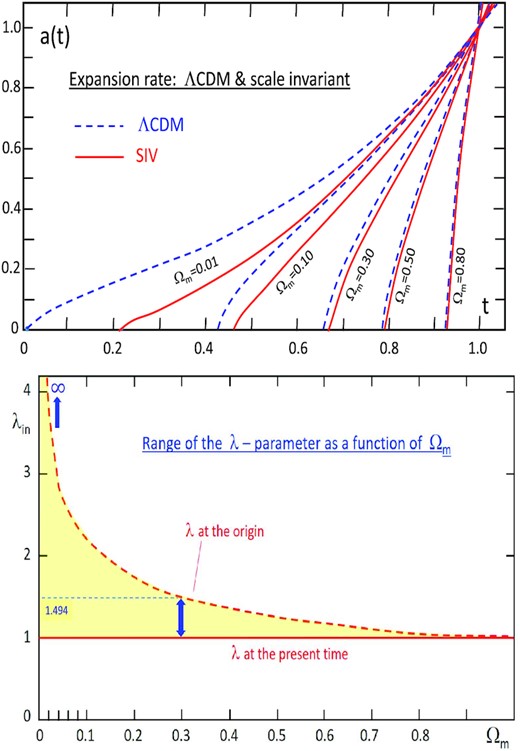
$Top: The expansion factor a(t) for the ΛCDM and SIV models as a function of Ωm. Bottom: The scale factor λin = 1/tin at the initial time $t_{\mathrm{in}}=\Omega ^{1/3}_{\mathrm{in}}$ as a function of Ωm. The yellow zone shows, versus Ωm, the range of λ(t) from the big bang (broken red line) to the present time (continuous red line). For Ωm = 0.3, λ(t) only varies between 1.494 at the origin and 1.0 at present.$

Figure 1.

Top: The expansion factor a(t) for the ΛCDM and SIV models as a function of Ω_m. Bottom: The scale factor λ_in = 1/t_in at the initial time |$t_{\mathrm{in}}=\Omega ^{1/3}_{\mathrm{in}}$| as a function of Ω_m. The yellow zone shows, versus Ω_m, the range of λ(t) from the big bang (broken red line) to the present time (continuous red line). For Ω_m = 0.3, λ(t) only varies between 1.494 at the origin and 1.0 at present.

Open in new tab Download slide

The initial time when a(t_in) = 0 is,

$$ \begin{eqnarray*} t_{\mathrm{in}} = \Omega ^{1/3}_{\mathrm{m}} . \end{eqnarray*} $$

(52)

This dependence in 1/3 produces a rapid increase of t_in for increasing Ω_m. For Ω_m = 0, 0.01, 0.1, 0.3, 0.5, the values of t_in are 0, 0.215, 0.464, 0.669, 0.794, respectively. The key point is that this leads to a strong reduction of the range of λ(t) for increasing Ω_m (Fig. 1, bottom): while the range of λ is infinite for an empty model, it is very limited for significant Ω_m-values.

Thus, the presence of matter through Ω_m drastically reduces the range of variation of the universal scale factor λ. For Ω_m > 1, scale invariance is killed which makes sense in view of the remarks by Feynman (1963). This is a global effect associated to the range of λ in the Universe models. This does not prevent other effects due to local variations of density to also intervene, as shown in Section 4.3, see equation (74).

The Hubble parameter is, in the time-scale t (which goes from t_in at big bang to t₀ = 1 at present),

$$ \begin{eqnarray*} H(t) = \frac{2 t^2}{t^3- \Omega _{\mathrm{m}}} . \end{eqnarray*} $$

(53)

From equations (51) and (53), we see that there is no meaningful scale invariant solution for an expanding universe model with Ω_m equal or larger than 1. Thus, the model solutions are quite consistent with the causality relations discussed by Maeder & Gueorguiev (2021a).

One can also define

$$ \begin{eqnarray*} \Omega _{\mathrm{k}} = -\frac{k}{a^2 H_0^2} \quad \mathrm{and} \quad \Omega _{\lambda } = - \frac{2}{H_0} \left(\frac{\dot{\lambda }}{\lambda }\right)_0 = \frac{2}{ H_0 t_0} . \end{eqnarray*} $$

(54)

These are the normalized contributions versus ϱ_c, respectively, of the matter, space curvature, and scale factor λ. With these definitions, the first cosmological equation (48) leads to,

$$ \begin{eqnarray*} \Omega _{\mathrm{m}} + \Omega _{\mathrm{k}} + \Omega _{\lambda } = 1 . \end{eqnarray*} $$

(55)

These quantities are usually considered at the present time.

4 THE NEWTONIAN AND MOND APPROXIMATIONS

4.1 The weak field approximation

The scale invariant expression of the geodesic equation was derived by Dirac (1973), and also from an action principle by Bouvier & Maeder (1978), see Section 2.3. The weak field low velocity approximation has been obtained by Maeder & Bouvier (1979), see also Maeder (2017c),

$$ \begin{eqnarray*} \frac{{\rm d}^2 {\bf r}}{{\rm d}t^2} = - \frac{G_t M(t)}{r^2} \frac{{\bf r}}{r} + \kappa (t) \frac{{\rm d}{\bf r}}{{\rm d}t} , \end{eqnarray*} $$

(56)

in spherical coordinates. It contains an additional acceleration term in the direction of motion, the dynamical gravity. This term, proportional to the velocity, favours collapse during a contraction, and outwards motion if expansion.

The conservation law (equation 47) imposes for a dust universe a relation ϱa³λ = const., meaning that the inertial mass of a particle is not a constant and that it depends on the scale factor λ. We note that the non-constancy of mass is also a common situation in Special Relativity. Here, masses vary like M(t) = M(t₀)(t/t₀). Interestingly enough, rather than the inertial and gravitational mass, the gravitational potential |$\Phi =G M/r$| of an object, thus the field, appears as a more fundamental quantity, being scale-invariant through the evolution of the Universe. As an example for Ω_m = 0.3, the mass at the big bang was, |$M(t_{\mathrm{in}}) = \Omega _{\mathrm{m}}^{1/3} M(t_0)= 0.6694 \; M(t_0)$|⁠, the variations are smaller than 1 per cent over the last 400 million years (Section 4.2).

In the above cosmological models, the age t is t₀ = 1 at present and |$t_{\mathrm{in}} = \Omega ^{1/3}_{\mathrm{m}}$| at the origin. The usual time-scale τ in years or seconds is τ₀ = 13.8 Gyr at present (Frieman, Turner & Huterer 2008) and τ_in = 0 at the big bang. Thus, the relation between these ages is,

$$ \begin{eqnarray*} \frac{\tau - \tau _{\mathrm{in}}}{\tau _0 - \tau _{\mathrm{in}}} = \frac{t - t_{\mathrm{in}}}{t_0 - t_{\mathrm{in}}} , \end{eqnarray*} $$

(57)

expressing that the age fraction with respect to the present age is the same in both time-scales. This gives

$$ \begin{eqnarray*} \tau = \tau _0 \frac{t- \Omega ^{1/3}_{\mathrm{m}}}{1- \Omega ^{1/3}_{\mathrm{m}}}{\quad}\mathrm{and}{\quad} t = \Omega ^{1/3}_{\mathrm{m}} + \frac{\tau }{\tau _0} \big(1- \Omega ^{1/3}_{\mathrm{m}}\big) , \end{eqnarray*} $$

(58)

and for the derivatives,

$$ \begin{eqnarray*} \frac{{\rm d}\tau }{{\rm d}t} = \frac{\tau _0}{1-\Omega ^{1/3}_{\mathrm{m}}} , \quad \mathrm{and}{\quad}\frac{{\rm d}t}{{\rm d}\tau } = \frac{1-\Omega ^{1/3}_{\mathrm{m}}}{\tau _0} . \end{eqnarray*} $$

(59)

For larger Ω_m, time-scale t is squeezed over a smaller fraction of the interval 0 to 1.0, (which reduces the range of λ over the ages).

We need to convert the equation of motion (56) expressed with variable t into the usual time τ, equation (56) becomes

$$ \begin{eqnarray*} \frac{{\rm d}^2 {\bf r}}{{\rm d}\tau ^2} \left(\frac{{\rm d} \tau }{{\rm d}t}\right)^2 = - \frac{G_{\rm t} M(t)}{r^2} \frac{{\bf r}}{r} + \frac{1}{ t_\mathrm{in} + \frac{\tau}{\tau _0} (t_0-t_\mathrm{in})} \frac{{\rm d}\tau}{{\rm d}t} \frac{{\rm d}{\bf r}}{{\rm d}\tau } . \end{eqnarray*} $$

(60)

Here G_t is used to specify that the gravitational constant is expressed with time units t. In the τ-scale, the units of G are [cm³ · g⁻¹ s⁻²], thus, the correspondence is |$G_{\rm t}\left(\frac{{\rm d}t}{{\rm d}\tau}\right)^2 = G$|⁠. At present, the masses M(t₀) and M(τ₀) are evidently equal. At other epochs, the relation is,

$$ \begin{eqnarray*} M(t)= \frac{t}{t_0} M(t_0), \; \mathrm{thus}\ M(\tau)=\left[ \Omega ^{1/3}_{\mathrm{m}}+\frac{\tau }{\tau _0} \big(1- \Omega ^{1/3}_{\mathrm{m}}\big) \right] M(\tau _0). \nonumber\\ \end{eqnarray*} $$

(61)

Now, multiplying both members of equation (60) by |$\big(\frac{{\rm d}t}{{\rm d}\tau}\big)^2$|⁠, we get at time τ/τ₀,

$$ \begin{eqnarray*} \frac{{\rm d}^2 {\bf r}}{{\rm d}\tau ^2} = - \frac{G M(\tau)}{r^2} \frac{{\bf r}}{r} + \frac{1}{ t_\mathrm{in} + \frac{\tau }{\tau _0} (t_0-t_\mathrm{in}) } \frac{t_0-t_\mathrm{in}}{\tau _0} \frac{{\rm d}{\bf r}}{{\rm d}\tau } . \end{eqnarray*} $$

(62)

We define the numerical factor ψ,

$$ \begin{eqnarray*} \psi (\tau) = \frac{t_0-t_\mathrm{in}}{ t_\mathrm{in} + \frac{\tau }{\tau _0} (t_0-t_\mathrm{in}) } ; \; \mathrm{thus} \; \psi _0=\psi (\tau _0) =1-\Omega ^{1/3}_{\mathrm{m}} . \end{eqnarray*} $$

(63)

The modified Newton’s equation at present time τ₀ is then,

$$ \begin{eqnarray*} \frac{{\rm d}^2 {\bf r}}{{\rm d}\tau ^2} = - \frac{G M(\tau _0)}{r^2} \frac{{\bf r}}{r} + \frac{\psi _0}{\tau _0} \frac{{\rm d}{\bf r}}{{\rm d}\tau}. \end{eqnarray*} $$

(64)

The additional term, the dynamical gravity, which is generally extremely small (cf. equation 74), also depends on Ω_m: in an empty universe, ψ₀ = 1, the effect being maximum, while for Ω_m = 1, one consistently has ψ₀ = 0, scale invariance has no effect. For Ω_m = 0.30, 0.20, 0.10, and 0.05 one has ψ₀ = 0.331, 0.415, 0.536, and 0.632, which reduces the dynamical gravity.

4.2 The MOND approximation: first approach

Let us first examine how the scale factor λ(τ) and consequently the masses M(τ) are varying over the past. For the case Ω_m = 0.30 as an example over the last 100, 200 Myr, and 0.5 Gyr, the mass increase predicted by equation (61) amounts to a factor 1.0024, 1.0048, and 1.012, respectively. For Ω_m = 0.10, these values would be 1.0039, 1.0078, and 1.020.

Thus, for galaxies where the rotation periods are a few hundered millions years, we can consider that both λ and masses are constant with an accuracy equal or better than 1 per cent. Indeed, this is quite consistent with MOND, which is also known to be scale invariant with a constant scale factor λ (Milgrom 2015). Such an approximation is much less satisfactory for clusters of galaxies, where the time-scales, e.g. the crossing times, are of the order of a few Gyr.

With a constant λ, the coefficient |$\kappa = -\frac{\dot{\lambda }}{\lambda }$| is equal to zero and the dynamical gravity in equation (64) disappears. We are left with transformations r = λ r′ and t = λ t′ with a constant λ (and thus M) applied to the Newton equation expressed in the prime coordinates,

$$ \begin{eqnarray*} \frac{{\rm d}^2r^{\prime }}{{\rm d}t^{\prime 2}} = - \frac{GM}{r^{\prime }{^2}} \equiv g^{\prime }_{\rm N}. \end{eqnarray*} $$

(65)

The total acceleration g in system (r, t) becomes,

$$ \begin{eqnarray*} g = \frac{{\rm d}^2r}{{\rm d}t^2} = \frac{1}{\lambda } \frac{{\rm d}^2 r^{\prime }}{{\rm d}t^{\prime 2}} . \end{eqnarray*} $$

(66)

The Newtonian gravitational accelerations g_N and |$g^{\prime }_{\rm N}$| are related by,

$$ \begin{eqnarray*} g_{\rm N} \equiv - \frac{G M}{r^2} = - \frac{1}{\lambda ^2} \frac{G M}{r^{\prime 2}} \equiv \frac{1}{\lambda ^2} g^{\prime }_{\rm N}. \end{eqnarray*} $$

(67)

Equation (66) can thus be developed as follows,

$$ \begin{eqnarray*} g = \frac{{\rm d}^2r}{{\rm d}t^2} = \frac{1}{\lambda}\frac{{\rm d}^2r^{\prime}}{{\rm d}t^{\prime 2}} = \frac{1}{\lambda} g^{\prime }_{\rm N} = {\lambda } g_{\rm N} , \end{eqnarray*} $$

(68)

according to (67). This last relation also implies,

$$ \begin{eqnarray*} g = \frac{{\rm d}^2r}{{\rm d}t^2} = {\lambda} g_{\rm N} = \left(\frac{g^{\prime }_{\rm N}}{g_{\rm N}}\right)^{1/2} g_{\rm N} = \left(g^{\prime}_{\rm N} g_{\rm N}\right) ^{1/2} . \end{eqnarray*} $$

(69)

This is to be compared to the deep-MOND limit given by equation (1). We note a correspondence between constant a₀ and |$g^{\prime }_{\rm N}$|⁠. At this stage, we have no information on what kind of value should be used for |$g^{\prime }_{\rm N}$|⁠, and for what range of gravities it may apply. In a second approach below, we will get more information on these points. For now, we note that the approximation of constant λ and masses over a few hundred millions years in the scale invariant theory just leads to a form analog to the deep-MOND limit.

The constant a₀ is related to |$c H_0$| (Milgrom 1983, 2015). We may wonder why a constant considered as a universal constant, thus being the same at any time, should just be related to the present value H₀, see also (Milgrom 2020). This is highly suggestive that a₀, alike λ, is in fact time dependent, contrarily to MOND assumption, but in agreement with the scale invariant theory.

4.3 The MOND approximation: second approach

We may also derive the MOND behaviour at very low gravities from the equation of motion equation (64). The ratio x of the radial components of the dynamical gravity to the Newtonian one is given by,

$$ \begin{eqnarray*} x = \frac{\psi _0 \upsilon r^2}{\tau _0 GM}, \end{eqnarray*} $$

(70)

where υ is the radial component of the velocity. The ratio x may become larger than 1 in two particular cases:

1) In very early stages of the Universe, τ₀ is very small and favours a large dynamical acceleration |$(\psi \upsilon)/\tau _0$| in the sense of motion. This effect is likely to have favoured the early galaxy formation without the need of dark matter (Maeder & Gueorguiev 2019).

2) At large distances from a central body, the Newtonian gravity g_N may become smaller than |$(\psi \upsilon)/\tau _0$|⁠. This may typically occur in very wide binaries and in the outer layers of galaxies and clusters. This situation is favoured by the fact that both the deep-MOND Limit and SIV theory predict that the orbital velocities in two-body systems are independant of the orbital radius (Maeder & Bouvier 1979; Milgrom 2014b). Thus in both cases, larger orbital velocities may favour the dynamical acceleration |$(\psi \upsilon)/\tau _0$| in the outer layers of gravitational systems.

We use the fact that |$H_0= \frac{\xi }{\tau _0}$| and |$\varrho _{\mathrm{c}}= \frac{3 H_0^2}{8 \pi G}$| to express τ₀ in term of ϱ_c in equation (70). To obtain ξ, we use the following expression of the Hubble–Lemaître parameter (see Appendix),

$$ \begin{eqnarray*} H(\tau _0) = \frac{ 2}{1- \Omega _{\rm m}} \frac{\big(1-\Omega ^{1/3}_{\rm m}\big)}{\tau _0} , \end{eqnarray*} $$

(71)

$$ \begin{eqnarray*} {\rm thus}\ \xi = \frac{ 2 \big(1-\Omega ^{1/3}_{\rm m}\big) }{(1- \Omega _{\mathrm{m}})}. \end{eqnarray*} $$

(72)

The ratio ξ is about unity in the SIV theory for Ω_m = 0.10, 0.20, or 0.30, there one has ξ = 1.191, 1.038, or 0.945, respectively.

We consider a mass M spherically distributed in a radius r with a mean density ϱ and get,

$$ \begin{eqnarray*} x = \frac{\sqrt{2} \psi _0}{\xi } \bigg(\frac{\upsilon ^2}{(GM/r)}\frac{\varrho _{\rm c}}{\varrho } \bigg)^{1/2} . \end{eqnarray*} $$

(73)

Let us consider a two-body system formed by a massive central mass M and a test object of negligible mass, there the instantaneous equilibrium of forces determined by equation (64) along the radial direction is just |$\frac{\upsilon ^2}{r} = \frac{GM}{r^2}$|⁠, since the additional dynamical acceleration is in the direction of the motion.³ Thus, in external regions of galaxies where normally the motion should be mainly determined by the central mass concentration, the ratio x becomes

$$ \begin{eqnarray*} x = \frac{\sqrt{2} \psi _0}{\xi } \bigg(\frac{\varrho _{\mathrm{c}}}{\varrho } \bigg)^{1/2} . \end{eqnarray*} $$

(74)

For high values of the density ϱ with respect to the critical density, the x-parameter becomes negligible, and thus the gravity is just determined by the usual Newton Law.

At the edge of the sphere of radius r and mean density ϱ, the Newtonian gravity |$g_{\rm N}= (4/3) \pi G \varrho r$|⁠, so that we also have

$$ \begin{eqnarray*} x = \frac{\sqrt{2} \psi _0}{\xi } \bigg(\frac{g_{\mathrm{c}}}{g_{\mathrm{N}}} \bigg)^{1/2} , \end{eqnarray*} $$

(75)

where g_c is the mean gravity at the edge of a similar sphere having the critical density. Thus, the total gravity g given by the the first member of equation (64) is

$$ \begin{eqnarray*} g = g_{\mathrm{N}} + x g_{\mathrm{N}} = g_{\mathrm{N}}\left[1+ \frac{\sqrt{2} \psi _0}{\xi } \left(\frac{g_{\mathrm{c}}}{g_{\mathrm{N}}}\right)^{1/2} \right] . \end{eqnarray*} $$

(76)

Let us consider regions at large distances from the galactic centre, or in a binary system at large distances from the other body. There, the Newtonian gravity g_N, resulting from the attraction of the central or other body, can be counterbalanced by the gravity of external galaxies or other star systems so that the resulting g_N essentially vanishes, and x becomes bigger than 1 in large regions. When this happens, we get a total resulting gravity g behaving like,

$$ \begin{eqnarray*} g \rightarrow \frac{\sqrt{2} \psi _0}{\xi }(g_{\mathrm{c}}\, g_{\mathrm{N}})^{1/2} . \end{eqnarray*} $$

(77)

The numerical factor |$\frac{\sqrt{2} \psi _0}{\xi }$| becomes,

$$ \begin{eqnarray*} \frac{\sqrt{2} \psi _0}{\xi }= \frac{\sqrt{2} (1- \Omega ^{1/3}_{\rm m})}{H(\tau _0) \tau _0} = \frac{(1- \Omega _{\mathrm{m}})}{\sqrt{2}} , \end{eqnarray*} $$

(78)

where we have used equation (72) for ξ. For Ω_m = 0, 0.1, 0.2, 0.3, 0.5, one has |$\frac{\sqrt{2} \psi _0}{\xi }=$| 0.707, 0.636, 0.566, 0.495, 0.354. Thus, the weak field equation (64) leads to relation (77) equivalent to the deep-MOND limit |$g = \sqrt{a_0 \; g_{\mathrm{N}}}$|⁠. In this second approach, we may learn much more on the significance of a₀ and its numerical value.

4.4 The significance of the a₀-parameter

We have the correspondence

$$ \begin{eqnarray*} a_0 \Longleftrightarrow \frac{(1-\Omega _{\mathrm{m}})^2}{2} g_{\mathrm{c}} . \end{eqnarray*} $$

(79)

We may explicit the limiting value g_c in term of the critical density over the radius |$r_{\mathrm{H_0}}$| of the Hubble sphere, defined by |$n c = r_{\mathrm{H_0}} H_0$|⁠. There, n depends on the cosmological model. As an example, for the EdS model, n = 2, for SIV or ΛCDM models with Ω_m = 0.2–0.3, the initial braking and recent acceleration almost compensate each other, so that n ≃ 1. We get,

$$ \begin{eqnarray*} a_0 = \frac{(1-\Omega _{\mathrm{m}})^2}{2} \frac{4 \pi }{3} G\,\varrho _{\mathrm{c}}\, r_{\mathrm{H_0 }} = \frac{(1-\Omega _{\mathrm{m}})^2}{4} n c H_0 \end{eqnarray*} $$

(80)

$$ \begin{eqnarray*} \mathrm{or} \quad a_0 = \frac{n c (1-\Omega _{\mathrm{m}}) (1-\Omega ^{1/3}_{\mathrm{m}})}{2 \tau _0}. \end{eqnarray*} $$

(81)

The product |$c H_0$| is equal to 6.80 10⁻⁸ cm s⁻². For Ω_m = 0, 0.10, 0.20, 0.30, and 0.50, we get a₀ ≈ (1.70, 1.36, 1.09, 0.83, 0.43) · 10⁻⁸ cm s⁻², respectively. These values obtained from the SIV theory are remarkably close to the value a₀ about 1.2 |$\cdot 10^{-8}$| cm s⁻² derived from observations by Milgrom (2015).

Let us make several remarks on the a₀-parameter and its meaning:

1) The equation of the deep-MOND limit is reproduced by the SIV theory both analytically and numerically if λ and M can be considered as constant. This may apply to systems with a typical dynamical time-scale up to a few hundred million years.

2) Parameter a₀ is not a universal constant. It depends on the Hubble–Lemaître H₀ parameter (or the age of the Universe) and on Ω_m in the model universe, cf. equation (80). The value of a₀ applies to the present epoch.

3) Parameter a₀ is defined by the condition that x > 1, i.e. when the dynamical gravity (ψ₀υ)/τ₀) in the equation of motion (equation 64) becomes larger than the Newtonian gravity. This situation may occur over large regions at the edge of gravitational systems.

5 CONCLUSIONS

The basic properties of SIV and its relations with the scalar–tensor theories of gravity have been reviewed. Similarities and differences have been enlightened. The deep-MOND limit is found to be an approximation of the SIV theory for low enough densities and for systems with time-scales smaller than a few Myr.

SIV theory preserves the physical properties of GR and enlarges the group of symmetries by the inclusion of scale covariance (Dirac 1973). In fact, this also avoid the call to dark matter, and at the same time as shown by Fig. 1, the SIV theory predicts an accelerated expansion. Results of a number of cosmological and astrophysical applications have been quoted in the introduction.

Finally, while the present approach may for the moment look ‘non-standard’ or out of the main stream, we point out that the present work is not in contradiction with the following statement by Einstein (1949): ‘…the existence of rigid standard rulers is an assumption suggested by our approximate experience, assumption which is arbitrary in its principle’.

ACKNOWLEDGEMENTS

I express my gratitude to Dr. Vesselin Gueorguiev for many years of support and excellent collaboration.

DATA AVAILABILITY

No new data were generated or analyzed in this research.

Footnotes

See a 312 pages review by Clifton, Ferreira, Padilla, and Skordis on ‘Modified Gravity and Cosmology’ (Clifton et al. 2012)

In the original Weyl’s Geometry, this other space was not necessarily General Relativity, while in WIG it is always the case.

When one considers the average velocity dispersion in a long-time evolution, this type of relation does not necessarily hold any more (Maeder 2017c))

REFERENCES

Asencio

Banik

Mieske

Venhola

Kroupa

Zhao

2022

MNRAS

515

2981

Month:	Total Views:
January 2023	3
February 2023	29
March 2023	37
April 2023	40
May 2023	55
June 2023	57
July 2023	35
August 2023	72
September 2023	30
October 2023	49
November 2023	29
December 2023	26
January 2024	32
February 2024	8
March 2024	14
April 2024	23
May 2024	22
June 2024	16
July 2024	5
August 2024	7
September 2024	10
October 2024	14
November 2024	12
December 2024	5
January 2025	8
February 2025	8
March 2025	17
April 2025	13
May 2025	2

Article Contents

MOND as a peculiar case of the SIV theory

ABSTRACT

1 INTRODUCTION

2 THE BASIC THEORETICAL CONTEXT

2.1 Scalar–tensor versus cotensor theories

2.2 Weyl’s integrable geometry (WIG) and relation with scalar–tensor theories

2.3 The geodesic and the field equations

2.4 Fixing the gauge

3 COSMOLOGICAL SOLUTIONS AND THEIR IMPLICATIONS

4 THE NEWTONIAN AND MOND APPROXIMATIONS

4.1 The weak field approximation

4.2 The MOND approximation: first approach

4.3 The MOND approximation: second approach

4.4 The significance of the a0-parameter

5 CONCLUSIONS

ACKNOWLEDGEMENTS

DATA AVAILABILITY

Footnotes

REFERENCES

APPENDIX A: THE HUBBLE CONSTANT IN CURRENT UNITS

Citations

Views

Altmetric

Email alerts

Astrophysics Data System

Citing articles via

Latest

Most Read

Most Cited

This Feature Is Available To Subscribers Only

4.4 The significance of the a₀-parameter