


ABSTRACT
Most active galactic nucleus (AGN) spectra show a soft X-ray excess above the 2–10 keV power law extrapolation. A warm corona has been widely used to explain the excess, but its observed radiation flux in the actually physical environment has yet to be further studied. For the first time, we calculate the relativistic warm coronal flux under the finite disc-corona thickness in high-accretion-rate systems. The numerical results show that the warm coronal flux generally rises first and then drops with increasing inclination. The flux rise is more significant for a compact and low-temperature warm corona and can reach 1–2 dexes. Meanwhile, the flux drop is significant if and only if the warm corona is heavily obscured due to the finite thickness. Our model can successfully explain the soft excess variance and the X-ray weak fraction in a high-accretion-rate AGN sample. In conclusion, our study indicates that when fitting the soft X-ray spectra of AGNs, the relativistic inclination dependence of warm coronal flux is essential, especially for the high-accretion-rate systems with thick warm coronae.
1 INTRODUCTION
The X-ray spectral energy distribution of active galactic nuclei (AGNs) can be fitted by a power-law within 2–10 keV. However, when extrapolating the best fit down to soft X-ray (<2 keV), most of the objects show a smooth excess (‘soft excess’; SE; e.g. Walter & Fink 1993; Boissay, Ricci & Paltani 2016; Liu et al. 2017). While the origin of the power-law emission is well known as the Comptonization of disc photons in an optically-thin (τ ∼ 1), hot (kT ∼ 100 keV) plasma (‘hot corona’; Sunyaev & Titarchuk 1980; Haardt & Maraschi 1993), there are still two well known interpretations for the origin of the SE. One is that the SE could be produced by the ionized reflection of the hot coronal flux on the disc (Ross & Fabian 2005; Crummy et al. 2006). However, the ionized reflection model requires extremely and unusually high black hole spin, compact hot corona, and sometimes large disc densities to smear out the line emission by relativistic effects (Crummy et al. 2006; Jiang et al. 2018; García et al. 2019; Xu et al. 2021b). Moreover, many analyses of observations show that the correlation between the SE and reflection ratio is very weak (Mehdipour et al. 2011, 2015; Noda et al. 2013; Matt et al. 2014; Boissay et al. 2016; Porquet et al. 2018; Matzeu et al. 2020; Xu et al. 2021a). Therefore, many researchers prefer the alternative interpretation, which could always give an excellent fit: the formation of the SE is due to the Comptonization of disc photons in an optically-thick (τ ∼ 10-40), warm (kT ∼ 0.1-1 keV) plasma (‘warm corona’). The main limitation of this two-corona scenario is its unclearly physical and geometrical structures.
Recently the research on the physical model of the two-corona scenario has made significant progress. Done et al. (2012; hereafter D12) suggested that the Comptonization region is radially stratified from the original disc, and they constrained the boundary location by energy conservation. This model was immediately applied to analyse a large sample of AGNs (Jin et al. 2012a; Jin, Ward & Done 2012b), although its description of physical processes in warm corona is relatively rough. To obtain the radiation spectra of a physical structure, Petrucci et al. (2013, 2018, 2020) investigated the radiative transfer in a slab-like warm plasma over the whole disc, and they found that when the plasma is a grey atmosphere with pure scattering and the disc is passive, the calculated spectra are in good agreement with the observations. The ‘passive disc’ means all the energy is dissipated in the upper warm Comptonization layer, and the underlying disc only thermalizes emission from above. However, such an extended warm corona leads to difficulties in explaining the time scale of X-ray variability, which implies that the distance between the emission region of the SE and power-law emission is about 10 gravitational radii or even less (De Marco et al. 2013; Kara et al. 2016; Mallick et al. 2021). Kubota & Done (2018, 2019; hereafter KD) modified the D12 model by adopting the passive-disc model for the warm Comptonization region, and they preserved the cool outer disc. However, though KD extended the D12 model to the high-accretion-rate (near- to super-Eddington) system, they still assumed that the warm coronal flux is proportional to the cosine of observing inclination (cos i, the observing inclination is the included angle between the line of sight and the rotation axis of the disc). Indeed, KD considered the warm Comptonization region a non-rotating, flat disc in Euclidian spacetime. However, for the following reasons, the consideration is not suitable for a compact warm corona:
Firstly, the warm corona rotates very rapidly near a black hole (BH). Since the warm plasma is an upper layer on the disc, its rotatation speed should be close to the Keplerian velocity, which can reach c/2 (c is the speed of light) at the Innermost Stable Circular Orbit (ISCO) of a non-spinning BH. Such a high velocity leads to strong relativistic Doppler shifts of received photons for an edge-on observer. Secondly, spacetime around the BH is curved by gravity. The gravitational redshift and light bending, together with the relativistic Doppler effect, will significantly affect the observed spectra. These relativistic effects are the key to SE formation in the ionized reflection model. They should also be important in the warm corona model since the physical environment is the same. Thirdly, the underlying disc and the upper warm plasma may have a finite thickness. Some studies show that either strong magnetic fields or vertical outflows are needed to stabilize the system (Różańska et al. 2015; Gronkiewicz & Różańska 2020), which may lead to a thick plasma. In addition, for the high-accretion-rate system, the innermost region of the disc is known to be puffed up due to the radiation pressure (Abramowicz et al. 1988; Ohsuga et al. 2005), and one could expect that the pressure will also blow up the warm plasma.
Since the warm corona is a rapidly-rotating, probably-thick emitter in curved spacetime, the inclination dependence of the warm coronal flux should not be simply proportional to the cos i. For the majority of type 1 AGNs, their inclinations are expected to be within 0°–60°, and for a few sources, the inclinations are even higher (e.g. Marin 2016). Such a wide variation range of inclination implies that the difference between the local and the observed radiation fluxes must be considered. A detailed study on the relation between the inclination and SE strength will be helpful to further understand the statistical properties of the X-ray emissions in the surveys of AGNs and the behaviors of some specific AGNs.
In this work, we calculate the spectra of warm coronal radiation in the full relativistic frame. For the first time, we consider the finite disc-corona thickness in high-accretion-rate systems and focus on the inclination dependence of the warm coronal flux. The models and methods are introduced in Section 2. The numerical results are shown in Section 3. In Section 4, we use our numerical results to explain the X-ray radiation properties in the high-accretion-rate sample reported by Laurenti et al. (2022). Finally, in Section 5, we make a conclusion.
2 MODELS AND METHODS
2.1 Relativistic frame
The photon trajectories in Kerr spacetime can be derived from the analytical integration of the null-geodesics (Čadež, Fanton & Calvani 1998; Li et al. 2005), and we trace the photons from the observing plane to the emitting surface. We do not consider the returning radiation in our calculations.
In this work, we assume that the AGNs are in the local Universe, or the cosmological redshifts have been carefully removed. Under the assumption, the rest frame of the observer at infinity is just the rest frame of the host galaxy.
2.2 Accretion disc models
ISCO radii (|$\rho _{_{\rm ISCO}}$|) for some spins (a).
| a | 0 | 0.5 | 0.8 | 0.9 | 0.98 | 0.998 | |
| |$\rho _{_{\rm ISCO}}$| | 6 | 4.23 | 2.91 | 2.32 | 1.61 | 1.24 |
| a | 0 | 0.5 | 0.8 | 0.9 | 0.98 | 0.998 | |
| |$\rho _{_{\rm ISCO}}$| | 6 | 4.23 | 2.91 | 2.32 | 1.61 | 1.24 |
The length unit is the gravitational radius, rg = GM/c2.
Temperature profiles of the discs with |$a=0,\dot{M}=1,2\dot{M}_{\rm Edd}$| (hereafter M1, M2) and |$a=0.98,\dot{M}=1/4,1/2\dot{M}_{\rm Edd}$| (hereafter also M1, M2 if there is no confusion) are shown in the top panel of Fig. 1 (more data are listed in Appendix A), where the |$\dot{M}_{\rm Edd}$| are defined by equation (7). Notice that the T in high-spin cases (a = 0.98) does not drop at small ρ. This is because the inner boundary of a slim disc will gradually extend from the ISCO to the horizon when the accretion rate increases. Indeed, the spin can hardly affect the temperature profiles when the accretion rate is very high (|$\gtrsim 10\dot{M}_{\rm Edd}$|; Li et al. 2010; Kubota & Done 2019). For the moderately super-Eddington discs here, when the BH is rapidly spinning (a > 0.9), the ISCO radius (<2.32rg) is very small and the inner boundary has extended to near the horizon. In other words, the difference between the slim discs in high-spin cases is tiny since T does not drop near the horizon. However, the NT disc is still susceptible to the BH spin. We select a large spin (a = 0.98) rather than the extreme spin (a = 0.998) for comparison between the NT and slim cases, since most super-massive BHs do not spin that rapidly, especially for those with MBH > 108 M⊙ (Reynolds 2021).
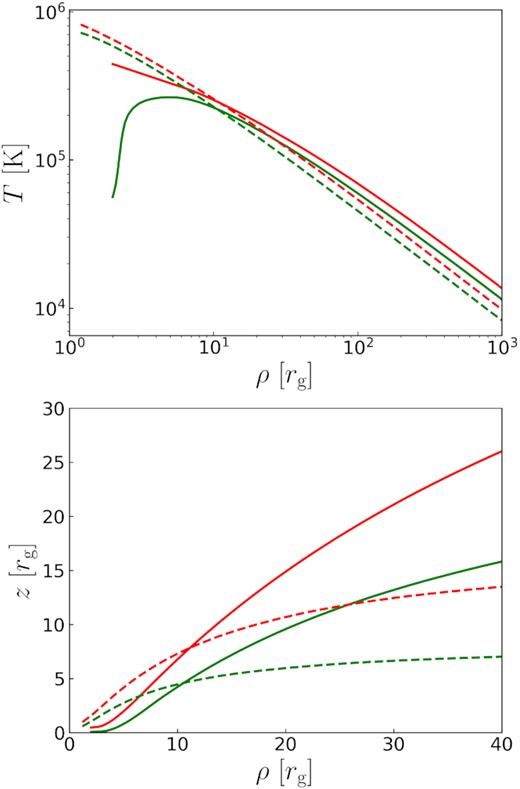
The temperature profiles (top) and geometries (bottom) of slim discs with different accretion rates. T is the temperature in unit of |$\rm K$|. ρ ≡ rsin θ is the cylindrical radius and z ≡ rcos θ is the height. Green, red colours correspond to the M1, M2 discs, respectively. Solid, dashed lines correspond to a = 0, 0.98, respectively. MBH = 107 M⊙.
We assume that on the disc surface, vr (the r-component physical velocity) is always much lower than vφ. For the pure disc solutions (NT and slim), this is a reasonable assumption outside the ISCO, since a test particle can rotate stably there. Meanwhile, simulations show that vr on the slim disc surface are not high within the ISCO (e.g. Sądowski et al. 2014; Jiang, Stone & Davis 2019a), then the assumption is applicable everywhere.
2.3 Corona model
In this work, our disc-corona structure follows the physical model developed by KD, but we further consider the disc-corona thickness (Fig. 2). The Comptonization region is radially stratified from the thermalization region at a cylindrical radius (ρout). Outside ρout, the accretion flow emits as a standard disc blackbody. Within ρout, the accretion flow has a vertical structure, there is a warm and optically-thick plasma (warm corona) covering and rotating with the accretion disc, and a hot corona which could either cover or truncate the innermost region of the disc and warm corona. We do not consider the hot coronal illumination or scattering in calculations since the hot coronal structure is still uncertain. Neglecting the hot corona leads to a small systematic error of the calculated warm coronal flux but hardly affects the inclination dependence.
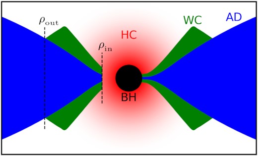
Sketch of our disc-corona model for calculations. BH (black): Black Hole; HC (red): Hot Corona; WC (green): Warm Corona; AD (blue): Accretion Disc. The hot corona covers (right) or truncates (left) the innermost region of the disc and warm corona. ρin, ρout are the cylindrical radii of the inner, outer boundary of the warm Comptonization region, respectively. In actual calculations, we do not consider the thickness of the warm coronae.
We calculate the local warm coronal spectral energy distribution by nthcomp (Zdziarski, Johnson & Magdziarz 1996; Życki, Done & Smith 1999). In the programme, the calculation of spectra needs three parameters:
Γ, asymptotic power-law photon index. Γ is related to the optical depth and electron temperature of the warm corona (Beloborodov 1999; Petrucci et al. 2018), and an SE usually have an apparent index at 2-3. We set Γ as 2, 2.5, 3 in this work.
kTe, electron temperature (high energy rollover). Since kTe of a warm corona is usually at 0.1-1 keV, we set kTe as 0.1, 0.3, 1 keV in this work.
kTbb, seed photon temperature. In this work it is just the local disc temperature (T). We use the NT solution TNT(ρ) for low-accretion-rate discs and our slim disc solution (shown in Fig. 1) for high-accretion-rate discs. The results weakly depend on kTbb as long as the observable band is far higher than the disc temperatures.
In this work, we calculate both the bolometric and observable warm coronal flux. When we say ‘bolometric flux’ in this paper, we always mean the radiant flux at all wavelengths, as measured by an ideal observer at infinity (e.g. our Galaxy). Notice that the cosmological redshift is not considered in calculations. The bolometric warm coronal flux is mainly contributed by the extreme UV (seed photon temperature level) to the soft X-ray (warm coronal temperature level) band. However, in actual observations, interstellar absorption from our Galaxy is heavy at low energy (≲ 0.3 keV), and only the high-energy tail (≳ 0.3 keV) is ‘observable’ for X-ray detectors. Spectral fitting is one way to reproduce the whole aspect from the observable flux (i.e. the SE), but the reproduction is model dependent and highly degenerate. Moreover, many observational works have yet to do a detailed analysis. Therefore, a phenomenological study of the observable flux is necessary. We set the observable band as 0.5-2 keV. The low energy is 0.5 (>0.3) keV because we reserve a margin for removing cosmological redshifts. The high energy is 2 keV because many observational works obtain the SE strength phenomenologically by removing the power-law component from the total flux below 2 keV.
The locally comoving warm coronal radiation intensity follows the Chandrasekhar formulae (table XXIV in Chandrasekhar 1960, see Appendix A), which is a limb-darkening law (very close to I(μ) ∝ 1 + 2.06μ, μ is the cosine of polar emission angle) due to an optically-thick, scattering-dominated atmosphere (Chandrasekhar 1960; Li, Narayan & McClintock 2009; Xiang et al. 2022). However, the μ variation becomes much more complicated after considering the finite thickness, and the obscuring effect is also essential (a further discussion will be given in Section 3). Therefore the results of a razor-thin disc (e.g. Xiang et al. 2022) can not be directly extrapolated to those of a thick disc. Meanwhile, the locally comoving disc radiation intensity is assumed to be isotropic.
To set up the numerical calculations, we still need to set the geometrical structures, including the thickness and boundaries of the warm corona. Since there is no complete theory to describe the warm corona thickness, we assume that the warm plasma is infinitely thin. The warm Comptonization region will still have a large apparent thickness if the underlying disc is thick.
The cylindrical radius of the inner boundary of the warm corona, ρin, depends on the hot coronal structure, which could either cover or truncate the innermost region of the disc and warm corona. For the covering structure, ρin should be the cylindrical radius of the inner boundary of the underlying disc. For the truncating structure, ρin should be the truncating radius. When KD constrained the truncating ρin by energy conservation, they did not consider the gravitational energy and rotation energy within the ISCO. However, under the action of magnetic fields, the energies play an important role in the formation and cooling of the hot corona (Blandford & Znajek 1977; Sądowski et al. 2014; Jiang et al. 2019b; Kinch et al. 2020), and thus ρin given by KD are very likely to be overestimated. Since KD also constrained ρout by energy conservation, larger ρin led to larger ρout. If fixing ρin at the ISCO, ρout will be close to the radii preferred by X-ray variability. Therefore, in this work, we set ρout in the region of ρin to 20rg.
3 NUMERICAL RESULTS
3.1 Schwarzschild cases
3.1.1 Bolometric warm coronal flux
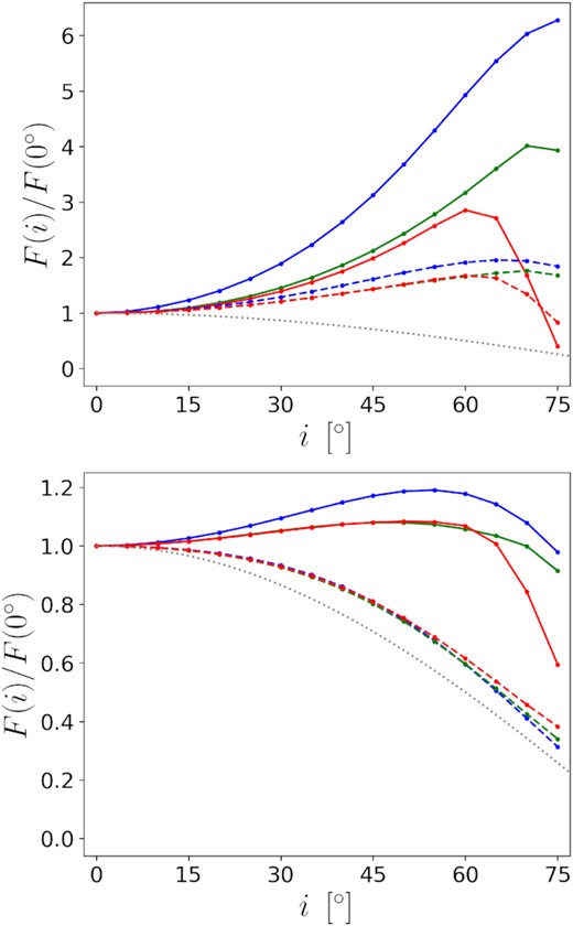
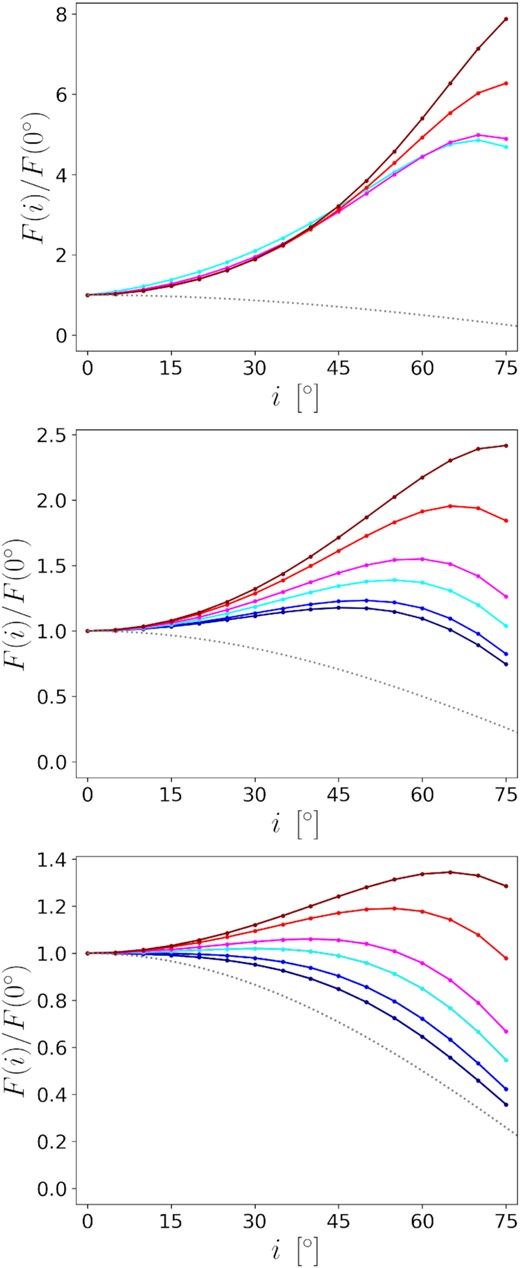
For a = 0, Fig. 3 shows the inclination (i) dependence of the bolometric warm coronal flux (|$F_{_{\rm WC}}$|, abbreviated as F if there is no confusion). Notice that there is no emission from the NT disc within the ISCO (|$\rho _{_{\rm ISCO}}=6$|). For compact warm coronae (ρout ≤ 10, top and middle panels), it is obvious that none of the curves has a cosine-like profile. To further understand this, we first briefly discuss the relativistic effects (see Appendix B for more details). In Kerr spacetime, the gravitational redshift mainly depends on the radius of the emitting location and only weakly depends on the inclination. Meanwhile, the radial velocity is positively correlated with the inclination. The relation means that the warm coronal flux will be more enhanced (or less weakened) by the relativistic Doppler effect at a higher inclination. In addition, the light-bending effect will reshape the projections of warm coronae and rearrange the weights of different radiation areas. When the inclination increases, the relativistic effects are generally against the non-relativistic decrease of warm coronal flux. The competition makes F rise first and then drop with increasing i, as shown in the top and middle panels of Fig. 3.
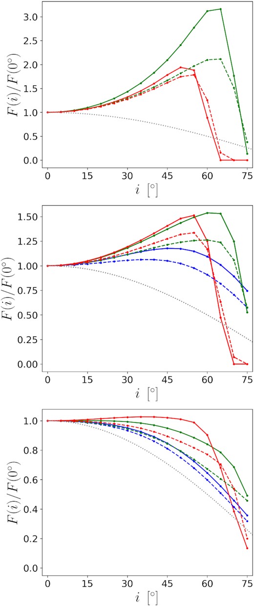
The bolometric warm coronal flux (F) as a function of the observing inclination (i). BH spin a = 0. Blue, green, red colours correspond to warm coronae on NT, M1, M2 discs, respectively. The grey curve indicates F = cos i. F is in unit of F(0°). Top: The outer boundaries of the warm coronae locate at ρout = 4 (solid) or 6 (dashed), and the inner boundaries are the same as those of the underlying discs. Middle: The same as the top panel but ρout = 8 (solid) or 10 (dashed). Bottom: The outer boundaries of the warm coronae locate at ρout = 20, and the inner boundaries are the same as those of the underlying discs (solid) or locate at ρin = 10 (dashed).
Although the relativistic effects determine the fundamental non-monotonic relation between F and i, the different disc-corona geometries lead to different details, such as the variation amplitudes and the transition inclinations (it, defined as where warm coronal flux takes the maximum value). For the simplest geometrical structure, i.e. the razor-thin warm coronae in the NT cases, the radial velocity could be high only if the inclination is high, but the effective area has dropped a lot at the same time. As a result, for the blue curves in the middle panel of Fig. 3, F can rise only a little with i. As a comparison, for the slim cases in the same panel, F increases faster with i at low inclinations and turn into a decrease at higher it. These changes are due to two geometrical differences between the slim discs and NT disc. One is that the slim discs keep their structure within the ISCO, at where the relativistic effects are strong. Another is that the slim discs are not razor-thin. Under the effect of light-bending, the thickness makes the discs turn edge-on much more quickly, which means that the radial velocities increase faster. However, the finite thickness of a slim disc also means that the outer disc obscures the inner warm corona for an edge-on observer. Thus F of a thicker warm corona drops much more dramatically at high inclinations. Heavy obscuration will also inverse the positive correlation between the transition inclination and disc thickness. As shown, the thicker slim disc (M2, red) begins to be obscured at a lower inclination.
The finite thickness causes one more phenomenon. When the emission area is very close to the BH (top panel of Fig. 3), the thicker disc (M2, red) still begins to be obscured at a lower inclination, but F of the thinner disc (M1, green) increases faster at low inclinations. The latter phenomenon is due to the lower physical rotational velocity at the surface of the thicker disc (see equation (13) and the discussions thereafter).
For the same disc, the scale of the warm corona is an important geometrical factor that can affect the results. In Fig. 3, among the curves of the same colour, the one for a smaller warm corona has a large maximum because the relativistic effects are stronger near the BH. For the same curve, the drop at large i is more significant because the proportion of obscured parts is larger. For extended warm coronae (ρout = 20, bottom panel of Fig. 3), it is obvious that the curve profiles are much more similar to the cosine curve than those of the compact coronae. It is because the strength of relativistic effects drops fast with increasing ρ, e.g. Keplerian velocity measured by a locally non-rotating observer in Schwarzschild spacetime is c/2 at the ISCO, and the velocity is only c/4 at ρ = 18rg. Therefore, one can expect that if ρout becomes even larger (several tens of rg), the results of the additional area will be even closer to the cosine profile. However, notice that the ‘cosine profile’ corresponds to a Newtonian disc emission without being limb-darkened. The profile in our results is due to the competition between the weak relativistic effects and limb-darkening effect. Therefore, when ρout is very large (e.g. a corona covering the whole disc), the curve profiles for the outer region should be closer to cos θ(1 + 2.06cos θ)/3.06.
The above study for the inclination dependence of bolometric warm coronal flux is helpful to study the structure of warm corona directly. However, since the warm coronal luminosity is proportional to the underlying disc luminosity, the relative strength of bolometric flux, χ, defined as the ratio of the bolometric warm coronal flux (|$F_{_{\rm WC}}$|) to the outer disc flux (|$F_{_{\rm AD}}$|), is more stable and useful in observations. Fig. 4 shows Ωi vs log χ for different warm coronae and discs, where Ωi ≡ 1 − cos i. The blue curves (NT) are monotonic increasing or very close to horizontal, because the warm coronal flux always suffers from stronger relativistic shifts than the disc flux due to the radially stratified structure. Meanwhile, only some green, red curves (slim) drop significantly at high inclinations, implying that the significant drop of χ will be and only be caused by heavy obscuration. Interestingly, for the slim discs, all the relations are very close to linear increases at low inclinations.
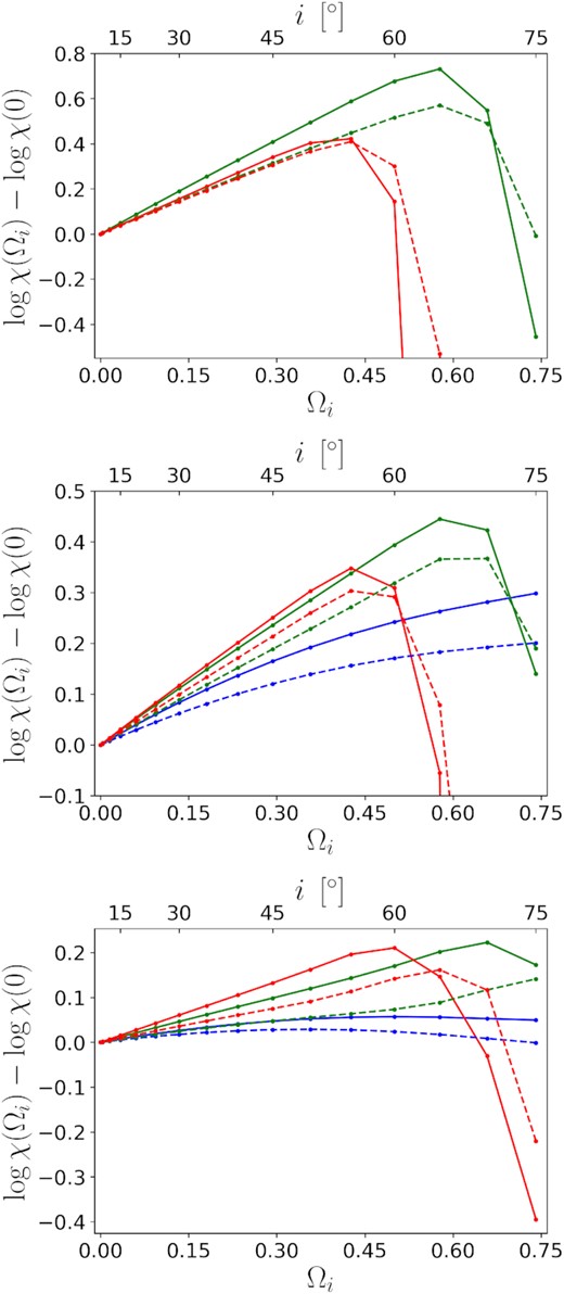
Ωi vs log χ for different warm coronae and accretion discs. |$\chi \equiv F_{_{\rm WC}}/F_{_{\rm AD}}$|, Ωi ≡ 1 − cos i, and i is the observing inclination. Blue, green, red colours correspond to warm coronae on NT, M1, M2 discs, respectively. Top: The outer boundaries of the warm coronae locate at ρout = 4 (solid) or 6 (dashed), and the inner boundaries are the same as those of the underlying discs. Middle: The same as the top panel but for ρout = 8 (solid) or 10 (dashed). Bottom: The outer boundaries of the warm coronae locate at ρout = 20, and the inner boundaries are the same as those of the underlying discs (solid) or locate at ρin = 10 (dashed).
3.1.2 Observable warm coronal flux
At first, we give a brief view of the observed spectra. Calculated spectra of two sets of parameters are shown in Fig. 5. The spectra with a high kTe (1keV) appear to follow a power-law distribution and show no cut-off, while the spectra with a low kTe (0.1keV) show a sharp drop. The total observable flux and apparent high energy rollover of the low kTe spectra increase with the inclination. Thus the spectra at high inclinations can easily be mistaken for those from extended and high-temperature warm coronae.
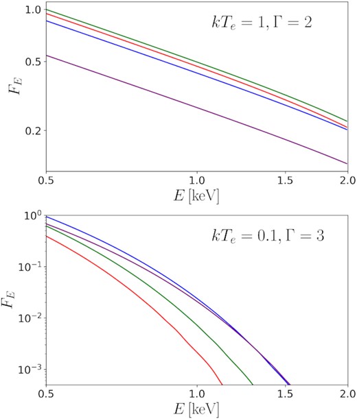
The observable spectra for a ρout = 10 warm corona on the NT disc at different inclinations. BH spin a = 0. FE are in arbitrary units. Γ and kTe are listed in each panel. The inclinations are 0° (red), 30° (green), 60° (blue), 75° (purple), respectively.
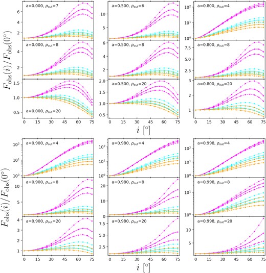
The calculation results for the integrated observable warm coronal flux (|$F_{_{\rm WC}}^{\rm obs}$|, abbreviated as Fobs if there is no confusion) as a function of the observing inclination (i) are shown in Figs 6 and 7. Unlike the bolometric flux F, Fobs is affected by the optical depth and electron temperature of the warm corona, i.e. Γ and kTe. Indeed, the relation F ∝ g4 is the same as the relation between g and Fobs of a power-law emission with Γ = 2 and without any cut-off (i.e. kTe ≫ 2 keV and kTbb ≪ 0.5 keV; see Appendix B for more details). Therefore, in these two figures, the dashed orange curves are most similar to the curves in Fig. 3. Meanwhile, in each panel of Figs 6 and 7, the dashed orange curve is at the bottom among all the curves, while the magenta curves (kTe = 0.1 keV) are at the top. For the most compact warm coronae (Fig. 7), the magenta curves can be up to tens to hundreds of times of Fobs(0°), while for the less compact ones (Fig. 6), the curves can be up to only a few times of Fobs(0°).
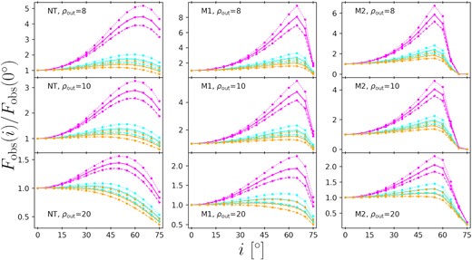
The integrated observable warm coronal flux (Fobs) as a function of the observing inclination (i). BH spin a = 0. The integration region is 0.5-2 keV, as measured by the distant observer. The electron temperature kTe = 0.1 (magenta), 0.3 (cyan), or 1 (orange), in unit of keV. The asymptotic power-law photon index Γ = 2.0 (dashed), 2.5 (solid), or 3.0 (dotted). The disc model and ρout are listed in each panel. All the warm coronae have the same inner boundary with the corresponding underlying discs.
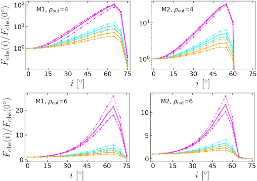
The same as Fig. 6 but for ρout = 4 or 6.
The large variation range of Fobs of the compact and low-temperature warm coronae indicates that the relativistic effects must be considered when fitting the SE, but the degeneracy of spectral profiles will make the fitting very difficult. One possible way to distinguish the degenerate spectra is to take advantage of statistical properties. In statistics, the relative SE strength (|$\chi _{\rm obs} \equiv F_{_{\rm WC}}^{\rm obs}/F_{_{\rm AD}}$|) is more useful. log χobs is linear correlated with Ωi at low inclinations, just like log χ vs Ωi. However, χobs is very sensitive to Γ and kTe, and |$F_{_{\rm AD}}$| is usually replaced by monochromatic flux in observations. Thus it is better to make a concrete analysis of each specific statistic (a case will be shown in Section 4).
3.2 High-spin cases
3.2.1 a = 0.98
Fig. 8 shows the inclination (i) dependence of the bolometric warm coronal flux (F) for a = 0.98. In general, when the spin is higher, the radiation will be more concentrated near the black hole. As a result, for all the compact warm coronae (top panel), the rises of F at low inclinations are faster than the corresponding ones (if there are) in Schwarzschild cases (Fig. 3), but the differences are not very obvious (i.e. still on the same order of magnitude). Indeed, the internal difference between the curves in the high spin case is even large. Among the blue curve (NT) and green, red curves (slim) in the top panel of Fig. 3, F in the slim cases increase more gradually with i because the finite thickness decreases the physical rotational velocity. For the extended warm coronae (bottom panel of Fig. 8), since the radiation from the innermost region is strong, F of the non-truncated warm coronae (solid) still increase at low inclinations. Meanwhile, a disc will be thinner at large radii if it is less puffed up by radiation there due to the concentration. As a result, the slim discs in high spin cases are less obscured, and the drops of F at high inclinations are not so significant.
The bolometric warm coronal flux (F) as a function of the observing inclination (i). BH spin a = 0.98. Blue, green, red colours correspond to warm coronae on NT, M1, M2 discs, respectively. The grey curve indicates F = cos i. F is in unit of F(0°). Top: The outer boundaries of the warm coronae locate at ρout = 4 (solid) or 8 (dashed), and the inner boundaries are the same as those of the underlying discs. Bottom: The outer boundaries of the warm coronae locate at ρout = 20, and the inner boundaries are the same as those of the underlying discs (solid) or locate at ρin = 10 (dashed).
The concentration of radiation will be more critical when considering the inclination (i) dependence of observable warm coronal flux (Fobs). As shown in Fig. 9, all the Fobs never significantly drop with increasing i, except for those in the right-hand panels (M2) at large i. It implies that when the spin is high, i.e. the radiation is largely concentrated, only heavy obscuration can make Fobs weak at high inclinations. In contrast, all the Fobs drop at high inclinations in a = 0 cases (Figs 6 and 7).

The integrated observable warm coronal flux (Fobs) as a function of the observing inclination (i). BH spin a = 0.98. The integration region is 0.5-2 keV, as measured by the distant observer. The electron temperature kTe =0.1 (magenta), 0.3 (cyan), or 1 (orange), in unit of keV. The asymptotic power-law photon index Γ = 2.0 (dashed), 2.5 (solid), or 3.0 (dotted). The disc model and ρout are listed in each panel. All the warm coronae have the same inner boundary with the corresponding underlying disc.
The above comparisons between results for different spins (a) are all carried out at the same ρout, but there has yet to be a conclusion for the correlation between a and ρout. For a specific relative SE strength (e.g. an actual one in observations), ρout decreases with increasing a, since the radiation is more concentrated at a higher spin. Therefore, a large variation of warm coronal flux with inclination will be more likely to correspond to a high spin (a further discussion will be given in Section 4).
3.2.2 More spins for the NT disc
Unlike the slim disc, the NT disc is truncated at the ISCO instead of extending to the horizon, and the ISCO radius is sensitive to the BH spin (equation 6 and Table 1). Therefore, F and Fobs of a warm corona on the NT disc are more susceptible to i when a is higher, as shown in Figs 10 and 11, respectively. It is clear that, for the same ρout, the variation range and transition inclination are positively correlated with a. Indeed, the curves for the higher spins (corresponding to the ISCOs closer to the horizon) are more similar to those for the slim discs. The results suggest that the inner boundary radius is one of the decisive factors affecting the inclination dependence of warm coronal flux. In contrast, the finite thickness can only moderately affect the rise of F and Fobs at low inclinations. However, a razor-thin disc will never be obscured at high inclinations. Thus in ideal NT cases, the drops of F and Fobs with increasing i are at most gradual, while there are significant drops due to obscuration by the finite thickness in slim cases. However, we should mention that an actual thin disc may have a thick warm Comptonization layer, since the warm coronal structure is still uncertain.
The bolometric warm coronal flux (F) as a function of the observing inclination (i). The underlying discs are the NT discs, the accretion rates are |$1/16\dot{M}_{\rm Edd}$| by definition equation (8). BH spin a = 0 (dark blue), 0.5 (blue), 0.8 (cyan), 0.9 (magenta), 0.98 (red), 0.998 (dark red), respectively. The grey curve indicates F = cos i. F is in unit of F(0°). The outer boundaries of the warm coronae locate at ρout = 4 (top), 8 (middle) or 20 (bottom). The inner boundaries are the corresponding ISCOs (notice that some ISCO radii are larger than 4).
The integrated observable warm coronal flux (Fobs) as a function of the observing inclination (i). The underlying discs are the NT discs, the accretion rates are |$1/16\dot{M}_{\rm Edd}$| by definition equation (8). The integration region is 0.5–2 keV, as measured by the distant observer. The electron temperature kTe =0.1 (magenta), 0.3 (cyan), or 1 (orange), in unit of keV. The asymptotic power-law photon index Γ =2.0 (dashed), 2.5 (solid), or 3.0 (dotted). The inner boundaries are the corresponding ISCOs. The BH spins and ρout are listed in each panel. Some ISCO radii are not smaller than 4 or 6, and thus the smallest ρout for different spin cases is not the same.
4 APPLICATION TO A HIGH-ACCRETION-RATE SAMPLE
The above systematic changes in AGN X-ray properties have yet to be completely clear. Meanwhile, it is hard to say how the BH mass affects the SE. For example, there is only sometimes an SE in the radiation spectra of X-ray binaries. Therefore, to apply our results to statistics of observations, it is better to find a sample of AGNs with λEdd and MBH each in a narrow interval. Fortunately, there is such an X-ray spectroscopic survey reported by Laurenti et al. (2022; hereafter L22), and we will discuss it further (we will keep the symbols consistent with L22 in the rest of this discussion). L22 presented the XMM-Newton (Jansen et al. 2001) observations of 14 AGNs from the large sample of high λEdd, radio-quiet, high-redshift (z ∼ 0.4–0.75) quasars provided by Marziani & Sulentic (2014). Furthermore, L22 required a clear broad Hβ emission line in the optical spectrum to constrain the BH mass. The 14 quasars are in narrow intervals of λEdd (∈ [0.9, 1.2]) and MBH/M⊙ (∈ [108, 108.5]), respectively. L22 found that four quasars are X-ray weak because their αox are obviously smaller than the αox vs LUV relation predicted (Lusso et al. 2010; Pu et al. 2020). L22 argued that the X-ray weakness is probably caused by the intrinsic variability of the hot corona, while scattering by highly-ionized, small-covering gas is also possible but unnatural. We then demonstrate that the latter scenario is a better interpretation and a natural result when considering the highly-ionized, small-covering warm corona.
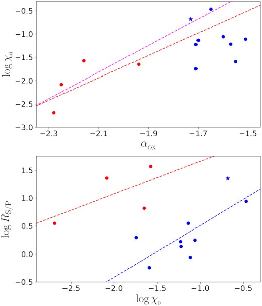
Top: |$\log \chi _{_{0}}$| vs αox for 13 of the 14 quasars reported in L22. Bottom: log RS/P vs |$\log \chi _{_{0}}$| for the same sample. One source (J0809+46) has been excluded since its spectrum shows no excess emission but a warm absorption in the soft X-ray band. Blue (X-ray normal), red (X-ray weak) lines are the best-fitting relations obtained from the linear regression analysis on all the circles and stars with corresponding colours, respectively, while magenta lines are obtained in the same way but from the blue stars (J1206 + 41) and red circles.
In addition, the Wilcoxon rank-sum test rejects the null hypothesis that RS/P of the X-ray weak and X-ray normal quasars are in the same distribution (p = 0.01). The average RS/P of the X-ray weak quasars is signifincantly larger, and the value is close to the largest RS/P of the X-ray normal quasars. The large RS/P means that the spectra of the X-ray weak quasars are quite soft, suggesting that the X-ray weakness is not due to heavy obscuration by cold absorption alone the line of sight, because the absorption will lead to a very hard X-ray spectrum (Morrison & McCammon 1983; Pu et al. 2020). The RS/P distribution will be a natural result if the X-ray weakness is due to the scattering by warm corona among the line of sight. In this scenario, the X-ray weak quasars evolve from the critical X-ray normal quasars, whose inclinations are close to the transition inclination it. The critical sources should have large RS/P, |$\chi _{_{0}}$| and small αox. J1206 + 41 (blue star) is a candidate for the critical quasars, since it has the smallest αox, largest RS/P and second largest |$\chi _{_{0}}$| among the X-ray normal quasars. Indeed, the blue star is neither close to the blue nor red line in the bottom panel of Fig. 12, probably due to some critical effects. For example, since the returning radiation usually has a large incident angle, most of the reflection will have a large reflection angle (Chandrasekhar 1960) and then escape (if not absorbed or scattered off) to observers near it. The reflection is also the probable reason for the gap (|$\chi _{_{0}}^{\rm g}\sim 0.4$|) in X-ray normal sources.
Fig. 13 shows the numerical results for |$\log \chi _{_{0}}$| vs Ωi(i) in the case of MBH = 1.6 × 10⁸M⊙ ≈ 108.2M⊙, M1 disc and a = 0, and Fig. 14 shows the results for a = 0.98. In L22, L/LEdd ∈ [0.9, 1.2], MBH/M⊙ ∈ [108, 108.5], and there may be some intrinsic variability (Δαox/0.384 ≃ 0.57). Moreover, we do not consider the warm coronal thickness here. Therefore, the two figures are just references. However, we can still obtain a large amount of valuable information from the numerical results:
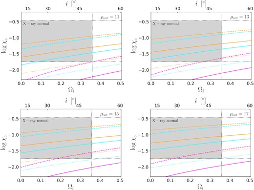
Numerical results for |$\log \chi _{_{0}}$| vs Ωi(i) in the case of MBH = 1.6 × 10⁸ M⊙ ≈ 108.2 M⊙, M1 disc, and a = 0. The electron temperature kTe =0.1 (magenta), 0.3 (cyan), or 1 (orange), in unit of keV. The asymptotic power-law photon index Γ = 2.0 (dashed), 2.5 (solid), or 3.0 (dotted). The corresponding ρout has been listed in each panel. The bottom and top horizontal lines correspond to the minimum and maximum |$\chi _{_{0}}$| of the X-ray normal quasars in L22, respectively. The vertical lines correspond to i = 50°. A good fit should be close to the bottom-left and top-right corners of the grey area at the same time.
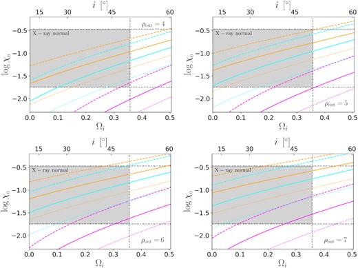
The same as Fig. 13 but for a = 0.98.
Firstly, for all the shown results, it (>60°) are larger than the one derived from equation (23) (50°). The difference implies that the warm corona does have a non-negligible extra thickness, as expected. For the sources within 50°–60°, the extra thickness makes them X-ray weak without showing any strong absorption features. The low it can explain why the fraction of X-ray weak quasars in the high-luminosity L22 sample (29 per cent) is larger than those in mixed-luminosity samples (e.g. 5.7 per cent in Pu et al. 2020). The detailed properties of the X-ray weak AGNs are susceptible to the actual structure of the warm corona, but the structure is still hard to determine. For example, the derived it (50°) is very close to 45°, the maximum opening angle of inflows (Sądowski & Narayan 2016; Feng et al. 2019, 2021), implying the existence of outflows.
Secondly, |$\Delta \chi _{_{0}}$| caused by the inclination change can be close to |$\Delta \chi _{_{0}}$| derived from L22. For the rapidly-spinning BH (a = 0.98; Fig. 14), there are some candidate results, such as the cyan dashed line (kTe =0.1, Γ =2.0) in the top right-hand panel (ρout = 4), the cyan solid line (kTe = 0.3, Γ = 2.5) in the top right-hand panel (ρout = 5), etc. Their |$\Delta \chi _{_{0}}$| are slightly smaller than the requirement, but the gap is very close to |$\chi _{_{0}}^{\rm g}$|, probably due to the returning rediation (not considered in the numerical calculations). However, for the non-spinning BH (a = 0; Fig. 14), none of the results fit the observations, since either the |$\Delta \chi _{_{0}}$| or the |$\chi _{_{0}}$| is too small. It is because while the large |$\Delta \chi _{_{0}}$| requires a small ρout, the radiation is not concentrated near the black hole in the Schwarzschild case, leading to a too large ρout to match the |$\chi _{_{0}}$|. The results prefer a large spin, but more is needed to make the conclusion. For example, besides the returning radiation, the magnetic fields can enhance the emission from the vicinity of BH (e.g. Agol & Krolik 2000), but they are not considered here.
Thirdly, the candidate warm coronae are compact (ρout < 10) and low-temperature (kTe ≤ 0.3). Compared with the other works, while the low temperature is a typical result, the compactness may be in debation. However, if a warm corona covers a large fraction of the disc (e.g. Petrucci et al. 2013, 2018, 2020), the appreciable UV emission from the Comptonization region will make |$L_{\nu }(2500 \mathring{\rm A})$| close to linearly correlating with the SE, but there is no such a correlation in L22. In addition, we notice that Matzeu et al. (2020) obtained a similar set of parameters, kTe ∼ 0.3 and ρout < 10, from the broadband spectral fitting of the super-Eddington (λEdd ∼ 5) AGN Ton S180. It seems that the warm coronae should be compact, at least in high-accretion-rate AGNs.
In the above analysis, we propose an ideal scenario in which all the quasars have the same intrinsic physical conditions and different inclinations. However, some independent intrinsic variabilities of warm coronal parameters and BH spin may exist. On the one hand, it is hard to believe that the similar quasars have very different physical conditions, and the variabilities can hardly explain the properties of the X-ray weak quasars. However, on the other hand, the variabilities can increase the uncertainties of estimated parameters. Further study is in need to estimate the uncertainties.
5 CONCLUSIONS
The warm corona has been widely used to explain the soft X-ray excess observed in the majority of AGNs. However, its observed radiation flux in the actual physical environment has yet to be further studied. In this work, we investigate the inclination dependence of warm coronal flux in AGNs. In calculations, we first obtain the local spectra of a warm Comptonization layer covering the innermost region of a given accretion disc. We consider the standard accretion disc and slim discs in our work. Then, for the first time, we obtain the observed spectra from the local spectra in the full relativistic frame under the finite disc-corona thickness in high-accretion-rate systems. From the numerical results, we find that the relativistic effects generally make the bolometric and observable warm coronal fluxes (F and Fobs, respectively) rise first and then drop with increasing inclination (i). The specific inclination dependence of the warm coronal flux directly depends on the geometrical and radiative properties of the warm corona:
the inner boundary (ρin) and outer boundary (ρout) of the warm corona. The rises of F and Fobs at low i are more significant for smaller ρin and/or smaller ρout, and may disappear in some ρout ≥ 20 cases.
the apparent thickness (z) of the warm corona. For the rises of F and Fobs at low i, large z moderately weakens or strengthens the rises for flux from small ρ (within a few rg) or large ρ, respectively. While for the drops of F and Fobs at high i, since large z makes the warm corona obscured, the drops are much more sinificant and begin at lower i. A significant drop can only caused by the obscuration.
the electron temperature (Te) of the warm corona. Te does not affect the bolometric flux F. In contrast, high Te enhances Fobs, the flux at high enengy (soft X-ray) band. For high Te (≈1keV), the difference between the inclination dependence of F and Fobs is very small. While for low Te (≤0.3keV), the rise of Fobs at low i is much more significant.
the asymptotic power-law photon index (Γ). Γ depends on the warm coronal temperature amd optical depth. Γ does not affect F, but the rise of |$F_{_{\rm WC}}^{\rm obs}$| at low i is moderately strengthened when Γ is larger.
Meanwhile, the BH and disc mainly indirectly affect the inclination dependence of the warm coronal flux:
the BH spin (a). High a decreases ρin (especially for low-accretion-rate discs) and concentrates the radiation near the black hole, and therefore strengthens the rises of F and Fobs at low i.
the accretion rate (|$\dot{M}$|). Large |$\dot{M}$| increases z, decreases ρin and concentrates the radiation near the black hole. Therefore, for high-accretion-rate systems, both the rises and drops of F and Fobs are more significant.
relative SE strength (χ). ρout, the boundary between the warm corona and disc, is far away from the BH for large χ. Therefore, for fainter warm coronae, the rises of F and Fobs at low i are more significant.
We successfully use our numerical results to explain the X-ray properties of the high-accretion-rate AGN sample reported by Laurenti et al. (2022). We find that the SE variance in the sample is a natural result of the uniform distribution of the quasars on the solid angle, and the variance prefers high BH spins (a > 0.9) in the sample. The X-ray weakness of four quasars in the sample is very likely due to the scattering by warm coronae rather than the intrinsic variability of hot coronae or the cold absorption. We find that the apparent thicknesses of the warm coronae are comparable to their cylindrical radii (|$z/\rho \sim \cot 50^{\circ }$|), suggesting an extra warm coronal thickness in high-accretion-rate systems.
In conclusion, when fitting the soft X-ray spectra of AGNs, the relativistic inclination dependence of warm coronal flux is essential, especially for the high-accretion-rate systems with thick warm coronae.
ACKNOWLEDGEMENTS
We thank Prof Jun-Xian Wang (University of Science and Technology of China) for proposals for this work. The first author also thanks Dr Si-Da Li (Brandeis University) for English writing. The work is partially supported by the National Natural Science Foundation of China (NSFC U2031201 and NSFC 11733001) and the Natural Science Foundation of Guangdong Province (2019B030302001). We acknowledge the science research grants from the China Manned Space Project, with NO. CMS-CSST-2021-A06. We also acknowledge support from Astrophysics Key Subjects of Guangdong Province and Guangzhou City, and support from Scientific and Technological Cooperation Projects (2020-2023) between the People’s Republic of China and the Republic of Bulgaria, as well as support that was received from Guangzhou University (No. YM2020001).
DATA AVAILABILITY
This is a theoretical paper that does not involve any new observational data. All the required data have been listed in this paper. The model data presented in this paper are all reproducible.
REFERENCES
APPENDIX A: DATA REQUIRED FOR CALCULATIONS
A1 Slim disc data
For MBH = 107M⊙, the slim disc data are listed in Table A1 (height) and Table A2 (temperature). For other MBH, one can use the same geometry and scale out the temperature by |$T\propto M_{\rm BH}^{-1/4}$|, e.g. T(1.6 × 10⁸ M⊙) = 0.5T(107 M⊙). The disc height varies very slowly at large radii, and the calculation results are not sensitive to the height there. Therefore, to save computing time, we approximate the disc height as a constant at large radii while keeping the disc shape smooth in cubic spline interpolation. The constant heights and critical cylindrical radii are shown in the last row of each column in Table A1.
Disc height (z) as functions of cylindrical radius (ρ).
| M1, a = 0 | M2, a = 0 | M1, a = 0.98 | M2, a = 0.98 | |
|---|---|---|---|---|
| ρ | z | z | z | z |
| 1.20 | 0.57 | 0.96 | ||
| 1.50 | 0.74 | 1.18 | ||
| 2.00 | 0.05 | 0.46 | 1.02 | 1.56 |
| 2.50 | 0.07 | 0.50 | 1.32 | 1.98 |
| 3.00 | 0.10 | 0.61 | 1.63 | 2.42 |
| 3.50 | 0.17 | 0.84 | 1.93 | 2.87 |
| 4.00 | 0.32 | 1.15 | 2.21 | 3.32 |
| 4.50 | 0.52 | 1.53 | 2.47 | 3.74 |
| 5.00 | 0.79 | 1.95 | 2.72 | 4.14 |
| 6.00 | 1.40 | 2.86 | 3.17 | 4.90 |
| 7.00 | 2.11 | 3.84 | 3.56 | 5.58 |
| 8.00 | 2.84 | 4.84 | 3.91 | 6.21 |
| 9.00 | 3.54 | 5.81 | 4.20 | 6.77 |
| 10.00 | 4.21 | 6.76 | 4.45 | 7.28 |
| 12.00 | 5.47 | 8.58 | 4.89 | 8.19 |
| 14.00 | 6.63 | 10.29 | 5.25 | 8.96 |
| 16.00 | 7.69 | 11.91 | 5.53 | 9.61 |
| 18.00 | 8.66 | 13.43 | 5.76 | 10.17 |
| 20.00 | 9.56 | 14.87 | 5.96 | 10.68 |
| 22.00 | 10.39 | 16.24 | 6.13 | 11.12 |
| 24.00 | 11.17 | 17.54 | 6.28 | 11.50 |
| 26.00 | 11.89 | 18.77 | 6.42 | 11.86 |
| 28.00 | 12.56 | 19.95 | 6.54 | 12.16 |
| 30.00 | 13.18 | 21.07 | 6.63 | 12.44 |
| 32.00 | 13.77 | 22.15 | 6.72 | 12.69 |
| 34.00 | 14.32 | 23.17 | 6.81 | 12.91 |
| 36.00 | 14.84 | 24.16 | 6.88 | 13.11 |
| 38.00 | 15.34 | 25.10 | 6.94 | 13.30 |
| 40.00 | 15.81 | 26.00 | 7.01 | 13.48 |
| >42.63 | 7.05 | |||
| >44.15 | 13.65 | |||
| 45.00 | 16.81 | 28.03 | ||
| 50.00 | 17.47 | 29.62 | ||
| 55.00 | 17.74 | 30.73 | ||
| >55.85 | 17.75 | |||
| 60.00 | 31.32 | |||
| >62.57 | 31.39 |
The length unit is rg.
Disc temperature (T) as functions of cylindrical radius (ρ).
| M1, a = 0 | M2, a = 0 | M1, a = 0.98 | M2, a = 0.98 | |
|---|---|---|---|---|
| ρ | T | T | T | T |
| 1.20 | 7.21 | 8.18 | ||
| 1.58 | 6.51 | 7.25 | ||
| 2.00 | 0.56 | 4.42 | 5.86 | 6.49 |
| 2.51 | 1.95 | 4.11 | 5.22 | 5.78 |
| 3.16 | 2.45 | 3.82 | 4.61 | 5.09 |
| 3.98 | 2.61 | 3.54 | 4.04 | 4.47 |
| 5.01 | 2.65 | 3.28 | 3.52 | 3.91 |
| 6.31 | 2.59 | 3.05 | 3.06 | 3.40 |
| 7.94 | 2.45 | 2.80 | 2.64 | 2.97 |
| 10.00 | 2.25 | 2.54 | 2.28 | 2.58 |
| 12.59 | 2.04 | 2.28 | 1.96 | 2.23 |
| 15.85 | 1.82 | 2.03 | 1.68 | 1.93 |
| 19.95 | 1.61 | 1.80 | 1.44 | 1.66 |
| 25.12 | 1.42 | 1.59 | 1.22 | 1.43 |
| 31.62 | 1.24 | 1.40 | 1.04 | 1.22 |
| 39.81 | 1.08 | 1.23 | 0.88 | 1.04 |
| 50.12 | 0.94 | 1.07 | 0.75 | 0.89 |
| 63.10 | 0.81 | 0.93 | 0.63 | 0.75 |
| 79.43 | 0.69 | 0.80 | 0.54 | 0.64 |
| 100.00 | 0.60 | 0.69 | 0.45 | 0.54 |
| 125.89 | 0.51 | 0.59 | 0.38 | 0.46 |
| 158.49 | 0.43 | 0.51 | 0.32 | 0.39 |
| 199.53 | 0.37 | 0.43 | 0.27 | 0.33 |
| 251.19 | 0.31 | 0.37 | 0.23 | 0.27 |
| 316.23 | 0.27 | 0.31 | 0.19 | 0.23 |
| 398.11 | 0.23 | 0.27 | 0.16 | 0.19 |
| 501.19 | 0.19 | 0.23 | 0.14 | 0.16 |
| 630.96 | 0.16 | 0.19 | 0.12 | 0.14 |
| 794.33 | 0.14 | 0.16 | 0.10 | 0.12 |
| 1000.00 | 0.11 | 0.14 | 0.08 | 0.10 |
T is in unit of 105K.
A2 Chandrasekhar formulae
|$I/\overline{I}$| as a function of μ.
| μ | 0 | 0.05 | 0.10 | 0.15 | 0.20 | 0.25 | 0.30 | 0.35 | 0.40 | 0.45 | 0.50 |
|---|---|---|---|---|---|---|---|---|---|---|---|
| |$I/\overline{I}$| | 0.41441 | 0.47490 | 0.52397 | 0.57001 | 0.61439 | 0.65770 | 0.70029 | 0.74234 | 0.78398 | 0.82530 | 0.86637 |
| μ | 0.55 | 0.60 | 0.65 | 0.70 | 0.75 | 0.80 | 0.85 | 0.90 | 0.95 | 1.00 | |
| |$I/\overline{I}$| | 0.90722 | 0.94789 | 0.98842 | 1.02882 | 1.06911 | 1.10931 | 1.14943 | 1.18947 | 1.22945 | 1.26938 |
The original data are from Table XXIV in Chandrasekhar (1960), and our ‘|$\overline{I}$|’ is marked as ‘F’ in that table.
A3 L22 data
In this paper, the required data are listed in Table A4, one source (J0809 + 46) has been excluded since its spectrum shows no excess emission but a warm absorption in the soft X-ray band.
Some data from L22.
| 1043 erg s−1 | eV | 1030 erg s−1 Hz−1 | |||||
|---|---|---|---|---|---|---|---|
| Obj. ID | z | |$\widetilde{R}_{\mathrm{S} / \mathrm{P}}$| | |$\widetilde{L}_{0.5-2 \mathrm{keV}}$| | kTbb | ΓPL | αox | |$L_{\nu }(2500 \mathring{\rm A})$| |
| J0300-08 | 0.562 | 1.24 | 0.94 | 140 | 1.9 | −2.28 | 5.78 |
| J0820 + 23 | 0.47 | 0.28 | 11.3 | 80 | 2.26 | −1.60 | 1.65 |
| J0940 + 46 | 0.696 | 2.59 | 67 | 134 | 2.3 | −1.65 | 4.66 |
| J1048 + 31 | 0.452 | 0.55 | 4.4 | 120 | 1.27 | −1.71 | 1.99 |
| J1103 + 41 | 0.402 | 2.42 | 6.9 | 122 | 1.6 | −1.94 | 4.33 |
| J1127 + 11 | 0.51 | 0.52 | 36 | 170 | 2.3 | −1.51 | 2.51 |
| J1127 + 64 | 0.695 | 4.37 | 2.4 | 110 | 1.5 | −2.16 | 3.99 |
| J1206 + 41 | 0.554 | 5.52 | 19.0 | 128 | 1.4 | −1.73 | 2.01 |
| J1207 + 15 | 0.75 | 0.45 | 39 | 160 | 2.0 | −1.57 | 5.1 |
| J1218 + 10 | 0.543 | 0.97 | 31 | 160 | 2.5 | −1.71 | 4.60 |
| J1245 + 33 | 0.711 | 2.93 | 2.6 | 120 | 1.3 | −2.25 | 10.5 |
| J1301 + 59 | 0.476 | 1.25 | 70 | 122 | 2.01 | −1.70 | 12.58 |
| J1336 + 17 | 0.552 | 0.10 | 60 | 100 | 1.86 | −1.55 | 9.49 |
In L22, ΓPL was mentioned as Γ, and |$\widetilde{R}_{\mathrm{S} / \mathrm{P}}$|, |$\widetilde{L}_{0.5-2 \mathrm{keV}}$| did not have the top tilde.
APPENDIX B: RELATIVISTIC EFFECTS
An emitter will project on the observing plane, and each point on the projection will correspond to a redshift. Some typical distributions of the warm coronal effective area (Ae) on g are shown in Fig. B1. It is worth noting that the distributions depend only on the warm coronal geometries and are independent of the local radiation properties. From the top panel (i = 15°), one can find that all the profiles are cut off at where g ∼ 0.9. At a low inclination, the Doppler blue shift caused by radial velocity is much smaller than the red shifts caused by the gravitational redshift and transverse redshift (transverse redshift is due to ‘moving clock running slow’), and therefore all the photons are red-shifted. From the middle panel (i = 60°), one can find that all the profiles show a double-peak feature. This is because the radial velocities are large enough to blue-shift some photons. From the bottom panel, one can find that the total Ae of green, red profiles (M1, M2) drop significantly due to obscuration. However, for the NT disc, |$A_{\rm e}(75^{\circ })/A_{\rm e}(15^{\circ })=41.1{{\ \rm per\, cent}}$|, larger than |$\cos 75^{\circ }/\cos 15^{\circ }=26.8{{\ \rm per\, cent}}$|, implying that the light-bending is more effective at the higher inclination. In conclusion, when the inclination increases, the relativistic effects are generally against the non-relativistic decrease of warm coronal flux.
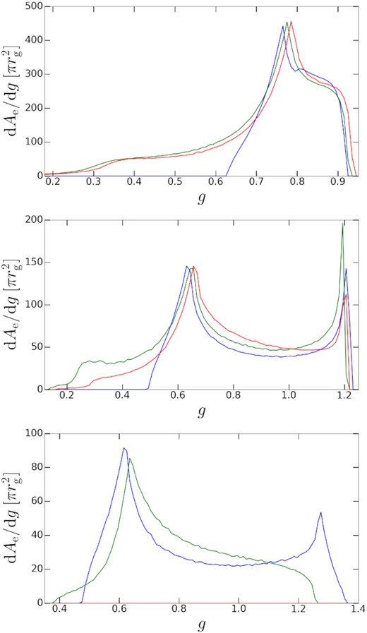
Effective area density (dAe/dg) of warm coronae as a function of redshift (g). Observing inclination i = 15° (top), 60° (middle), or 75° (bottom). BH spin a = 0. The outer boundaries of warm coronae locate at 10rg. Blue, green, red colours correspond to warm coronae on NT, M1, M2 discs, respectively. Ae is in unit of |$\pi r_{\rm g}^2$|.
