


ABSTRACT
We report new, extremely precise photopolarimetry of the rapidly-rotating A0 main-sequence star ζ Aql, covering the wavelength range ∼400–900 nm, which reveals a rotationally-induced signal. We model the polarimetry, together with the flux distribution and line profiles, in the framework of Roche geometry with ω-model gravity darkening, to establish the stellar parameters. An additional constraint is provided by TESS photometry, which shows variability with a period, Pphot, of 11.1 h. Modelling based on solid-body surface rotation gives rotation periods, Prot, that are in only marginal agreement with this value. We compute new ester stellar-structure models to predict horizontal surface-velocity fields, which depart from solid-body rotation at only the ∼2 per cent level (consistent with a reasonably strong empirical upper limit on differential rotation derived from the line-profile analysis). These models bring the equatorial rotation period, Prot(e), into agreement with Pphot, without requiring any ‘fine tuning’ (for the Gaia parallax). We confirm that surface abundances are significantly subsolar ([M/H] ≃ −0.5). The star’s basic parameters are established with reasonably good precision: |$M = 2.53\pm 0.16\, \mbox{M}_{\odot }$|, log (L/L⊙) = 1.72± 0.02, |$R_{\rm p}= 2.21\pm 0.02\, \mbox{R}_{\odot }$|, Teff = 9693 ± 50 K, |$i = 85{^{+5}_{-7}}^\circ$|, and ωe/ωc = 0.95 ± 0.02. Comparison with single-star solar-abundance stellar-evolution models incorporating rotational effects shows excellent agreement (but somewhat poorer agreement for models at [M/H] ≃ −0.4).
1 INTRODUCTION
The discovery of rotationally-induced wavelength-dependent linear polarization in Regulus (α Leo; Cotton et al. 2017a) unveiled a new tool for investigating the properties of rapid rotators, opening the possibility of reasonably precise determinations of mass (and other parameters) in single stars. Subsequent studies have shown that high-quality photopolarimetry can afford powerful tests of stellar-atmosphere physics and of evolutionary models incorporating rotation (Bailey et al. 2020b; Lewis et al. 2022).
Here, we examine new results for ζ Aql (HD 177724, HR 7235, ‘Okab’), to explore further the diagnostic potential of very precise photopolarimetry. Selected basic data for the star are assembled in Table 1, including some of the observational material reviewed in Section 2. Section 3 outlines our modelling procedures. Results are given in Section 4, which examines the question of possible differential surface rotation. Section 5 confronts the inferred stellar parameters with stellar-evolution models. The determination of vesin i, and other aspects of the line-profile analysis, are relegated to Appendix B.
Selected basic observational data.
| Parameter | Value | Source |
|---|---|---|
| Spectral type | A0 IV–Vnn | Gray et al. (2003) |
| Parallax | 39.28 ± 0.16 mas | van Leeuwen (2007) |
| 38.23 ± 0.35 mas | Gaia Collaboration (2021a,b) | |
| vesin i | 306|$^{+20}_{-5}$| km s−1 | Section 2.3.3, Appendix B |
| V | 2.99 | Johnson et al. (1966) |
| 2.98 | Häggkvist & Oja (1969) | |
| E(B − V) | 0|${_{.}^{\rm m}}$|005 | Section 2.3.2 |
| f(123.5–321nm) | 4.76 × 10⁻⁷ | Section 3.2.1 |
| erg cm−2 s−1 | ||
| Interferometric results: | ||
| |$\overline{\theta }$| | 0.895 ± 0.017 mas | Boyajian et al. (2012) |
| 0.961 ± 0.007 mas | Peterson et al. (2006) | |
| ωe/ωc | 0.990 ± 0.005 | (but see Section 5) |
| i | |$90_{-5}^{+0\, \circ }$| | ” |
| θ* | 45 ± 5○ | ” |
Note.|$\overline{\theta }$| is the geometric mean of the major- and minor-axis limb-darkened angular diameters; θ* is the position angle of the stellar rotation axis, which is at an angle i to the line of sight.
2 OBSERVATIONS
2.1 Photopolarimetry
The new observations reported here were obtained using HIPPI, the HIgh-Precision Polarimetric Instrument, and its successor, HIPPI-2; the design and operation of these instruments are described by Bailey et al. (2015, 2020a). We also made use of one previously published observation (Bailey, Lucas & Hough 2010), obtained using PlanetPol (Hough et al. 2006).
Details of observing runs and instrument configurations are given in Appendix A (Table A1), and the individual observations of ζ Aql are listed in Table 2. As well as shot noise, the uncertainties reported therein on the normalized Stokes parameters q, u, and on the polarization p, include (in quadrature) a wavelength-dependent positioning error which results from inhomogeneities across the face of the ferroelectric liquid-crystal modulator, and which sets the accuracy limit for the instruments. For HIPPI-2, this limit ranges from 1.1 parts per million (ppm) for the reddest passbands, through 2.5 ppm in g′, to 13.7 ppm in the 425SP filter – similar to, but slightly better than, the corresponding figures for HIPPI (Bailey et al. 2020a). Position-angle (PA) calibration was performed using highly-polarized standard stars; typical PA zero-point uncertainties are ∼1 ○ (i.e. are smaller than the statistical errors on our measurements).
Photopolarimetry of ζ Aql, sorted by passband effective wavelength, λeff. Run identifiers correspond to entries in Table A1, where further technical details are given, and reflect the year and month of each observing campaign. Dwell times include observing overheads, and so exceed actual integration times (‘Int.’). ‘Det.’ indicates whether a B(lue) or R(ed) photomultiplier tube was used as detector; ‘Eff.’ is the modulator polarization efficiency. The final four columns give the normalized Stokes parameters, q, u; the polarization, p; and the observed polarization position angle, θp (where q = Q/I = pcos 2θp, u = U/I = psin 2θp, and 0○ ≤ θp < 180○).
| Run ID | MJD | Dwell | Int. | Filter | Det. | λeff | Eff. | q | u | p | θp |
|---|---|---|---|---|---|---|---|---|---|---|---|
| (mid-dwell) | (s) | (s) | (nm) | (%) | (ppm) | (ppm) | (ppm) | (○) | |||
| 2017_08 | 57 977.530 | 3458 | 2560 | 425SP | B | 400.7 | 52.2 | 20.6 ± 14.5 | −12.0 ± 14.5 | 23.8 ± 14.5 | 164.9 ± 21.6 |
| 2018_07 | 58 318.566 | 1426 | 960 | 425SP | B | 402.7 | 38.3 | 58.0 ± 16.0 | −16.7 ± 15.8 | 60.4 ± 15.9 | 172.0 ± 7.7 |
| 2018_07 | 58 315.473 | 1077 | 640 | 425SP | B | 403.0 | 38.5 | 43.7 ± 17.1 | −2.8 ± 16.8 | 43.8 ± 17.0 | 178.2 ± 12.5 |
| 2017_08 | 57 977.569 | 1870 | 640 | 500SP | B | 436.9 | 75.4 | 36.2 ± 9.1 | −0.9 ± 9.4 | 36.2 ± 9.3 | 179.3 ± 7.5 |
| 2018_07 | 58 318.525 | 1058 | 640 | 500SP | B | 438.5 | 67.1 | 20.2 ± 7.4 | −12.1 ± 7.3 | 23.5 ± 7.4 | 164.5 ± 9.4 |
| 2018_07 | 58 315.459 | 1132 | 640 | 500SP | B | 439.5 | 67.9 | 13.0 ± 7.3 | −1.9 ± 7.4 | 13.1 ± 7.4 | 175.8 ± 19.9 |
| 2018_07 | 58 318.511 | 1161 | 640 | g′ | B | 462.8 | 79.6 | 12.7 ± 3.9 | −4.7 ± 3.6 | 13.5 ± 3.8 | 169.8 ± 8.1 |
| 2015_10 | 57 314.382 | 1238 | 640 | g′ | B | 464.8 | 89.4 | 39.3 ± 4.3 | −1.3 ± 4.3 | 39.3 ± 4.3 | 179.1 ± 3.2 |
| 2017_08 | 57 977.569 | 2610 | 640 | g′ | B | 464.8 | 86.9 | 21.5 ± 4.7 | 1.2 ± 5.1 | 21.5 ± 4.9 | 1.6 ± 6.7 |
| 2018_07 | 58 318.551 | 1067 | 640 | V | B | 532.3 | 95.6 | 8.6 ± 5.4 | −6.3 ± 5.1 | 10.7 ± 5.3 | 161.9 ± 17.1 |
| 2018_07 | 58 315.445 | 1039 | 640 | V | B | 532.8 | 95.6 | −1.8 ± 5.6 | 6.8 ± 5.5 | 7.0 ± 5.6 | 52.4 ± 27.3 |
| 2018_07 | 58 318.538 | 1066 | 640 | r′ | B | 601.9 | 86.8 | −4.2 ± 9.3 | 1.0 ± 8.8 | 4.3 ± 9.0 | 83.3 ± 42.1 |
| 2018_07 | 58 315.432 | 1033 | 640 | r′ | B | 602.3 | 86.8 | −2.8 ± 10.1 | 1.5 ± 9.6 | 3.2 ± 9.8 | 75.9 ± 45.3 |
| 2017_08 | 57 973.533 | 3551 | 2560 | r′ | R | 619.5 | 82.6 | 6.3 ± 3.4 | 18.2 ± 3.3 | 19.3 ± 3.4 | 35.5 ± 5.0 |
| 2018_07 | 58 322.569 | 2508 | 960 | r′ | R | 621.2 | 83.1 | −0.3 ± 3.9 | 14.0 ± 3.9 | 14.0 ± 3.9 | 45.6 ± 8.1 |
| 2017_08 | 57 973.492 | 3404 | 2560 | 650LP | R | 717.7 | 65.9 | −11.5 ± 5.4 | 14.4 ± 5.4 | 18.4 ± 5.4 | 64.3 ± 8.7 |
| 2018_07 | 58 322.602 | 1439 | 640 | 650LP | R | 721.0 | 65.0 | −1.9 ± 9.6 | 33.6 ± 9.7 | 33.7 ± 9.6 | 46.6 ± 8.4 |
| 2005_04a | 53 494.216 | 1830 | 1440 | BRB | APD | 745.4 | 92.3 | −13.0 ± 3.7 | 18.7 ± 3.7 | 22.8 ± 3.7 | 62.4 ± 4.7 |
aThe PlanetPol observation comes from Bailey et al. (2010).
Results are plotted in Fig. 1; the scatter in the observations slightly exceeds the quoted formal errors (though is still small compared to results from traditional polarimeters), as was also found in our study of θ Sco (Lewis et al. 2022). Although intrinsic low-level polarization variability cannot be ruled out, the scatter is consistent with a combination of instrument-configuration changes and imperfect characterization of low-polarization standard stars (used to correct for polarization arising in the telescope optics), which can lead to zero-point drifts of up to ∼10 ppm between runs (Bailey et al. 2021). These factors are accommodated in our modelling by use of bootstrapping in the error analysis (Section 4).
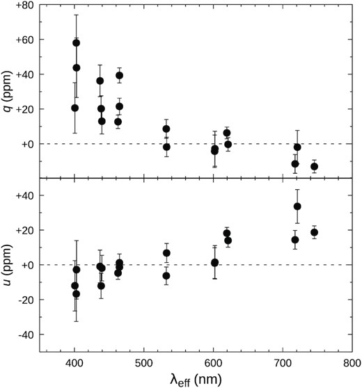
Observed photopolarimetry of ζ Aql.
2.2 TESS photometry
The TESS satellite (Ricker et al. 2015) observed ζ Aql in sector 54 (2022 July–August). The light-curve is shown in Fig. 2; a periodic signal is immediately evident. A generalized Lomb–Scargle periodogram ( Ferraz-Mello 1981; Zechmeister & Kürster 2009) yields a fundamental frequency and corresponding semi-amplitude of
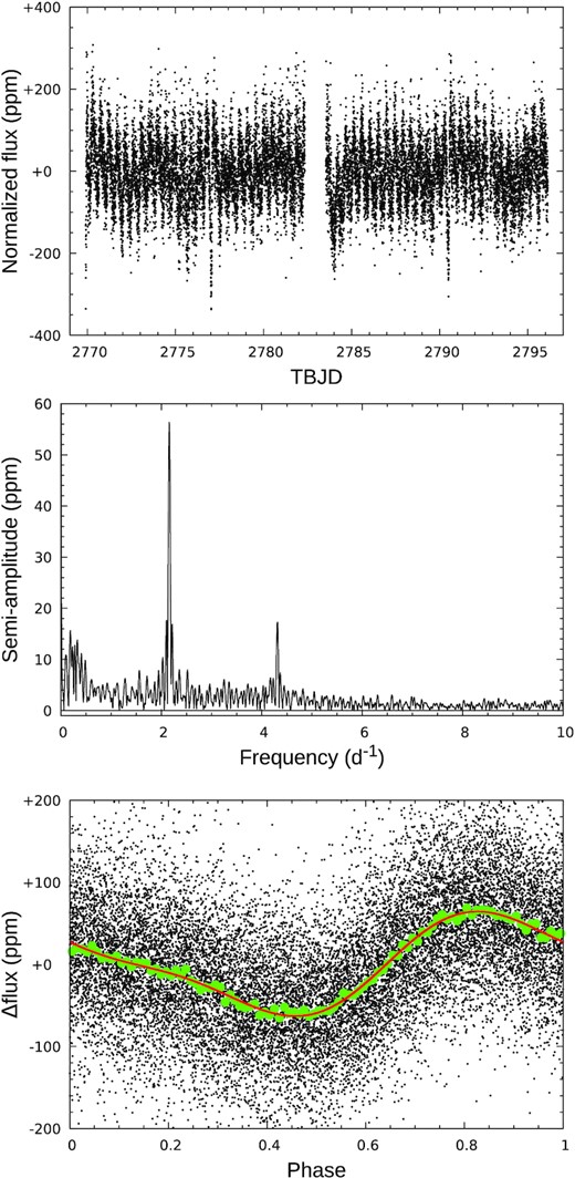
TESS light-curve of ζ Aql. Top panel: PDCSAP flux (‘pre-search data conditioning simple aperture’, normalized simply by dividing the mean and subtracting unity) as a function of TESS Barycentric Julian Date (|$=\text{BJD} - 2\, 457\, 000.0$|, |$\simeq \text{MJD} - 56\, 999.5$|). Middle panel: generalized Lomb–Scargle periodogram. Bottom panel: photometry phase-folded at Pphot = 11.118 h (with phase zero arbitrarily defined as time of first observation); green dots are data averaged in 0.01 phase bins, and the red line is the two-component Fourier model.
|$\phantom{X} \nu _0= 2.1587 (8)$| d−1 [Pphot = 11.118(4) h]
|$\phantom{X} a_0=56.5 (25)$| ppm
where parenthesized values are 1σ uncertainties on the least significant digits, generated from Monte Carlo simulations using a residual-permutation, or ‘prayer beads’, algorithm (adopted because the residuals are strongly correlated as a result of lower-frequency drifting). The signal appears to be rather simple; power at the first harmonic accounts almost entirely for departures from a pure sinusoid (Fig. 2).
2.3 Ancillary observational data
Some additional observational material is required for our analysis; furthermore, given the level of precision of the polarimetry, consideration needs to be given to potential contaminating sources (whether stellar or circumstellar).
2.3.1 Parallax
Parallaxes, required principally to establish the stellar radius, are available from both the Hipparcos and Gaia missions (van Leeuwen 2007; EDR3, Gaia Collaboration 2021a, b). The Hipparcos result is 1.05 ± 0.38 mas larger than the EDR3 value (Table 1), a 2.6σ difference. Although this difference is of little consequence for most derived parameters (cf. Table 4), it proves to be of some significance for the interpretation of the photometric period (Section 4.1). We therefore performed calculations for both values (taking the distance, ∼26 pc, to be simply the inverse of the parallax1).
2.3.2 Interstellar polarization and extinction
Cotton et al. (2017a) developed a model of interstellar polarization from which we expect p(λmax) ≃ 30 ppm for ζ Aql, where λmax is the wavelength of maximum linear polarization (typically ∼0.5 |$\mu$|m). Observations of stars over a range of distances in the general direction of ζ Aql support this estimate, with an upper limit of ∼50–60 ppm (Fig. 3). The interstellar polarization is directly estimated as part of the modelling (Section 3.1), and yields p(λmax ) ∼17–24 ppm (in position angle θi = 55 ± 2○), in good accord with the Cotton et al. model.
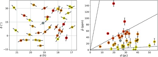
(Left) map and (right) bias-corrected polarization, |$\hat{\boldsymbol{ p}},$| versus distance d for interstellar control stars within 35○ and 30 pc of ζ Aql (which is indicated by the grey data points; in the right-hand panel, this is the prediction of the interstellar model of Cotton et al. 2017b). Distances and coordinates were obtained from SIMBAD (mostly Gaia DR3 values, with a handful of Hipparcos results), and polarization measurements from Bailey et al. (2010), Marshall et al. (2016), Piirola et al. (2020), and Bailey et al. (2020b), with two additional values from Marshall et al. (in preparation). Black pseudo-vectors on the map points indicate the position angles (but not the magnitudes) of the interstellar polarizations. For the d–|$\hat{\boldsymbol{ p}}$| plot, observed polarizations p were debiased using the method of Wardle & Kronberg (1974), as first discussed by Serkowski (1958): |$\hat{\boldsymbol{ p}} = \left({p^2-\sigma _p^2}\right)^{1/2}$| for p > σp, or |$\hat{\boldsymbol{ p}} = 0$| otherwise (which corrects for p being positive definite). We then transformed the multi-wavelength results to a standardized effective wavelength of 450 nm by adopting a Serkowski law (equation 2) with λmax = 470 nm, appropriate for stars within the Local Hot Bubble (Marshall et al. 2016; Cotton et al. 2019), and K set by equation (3). Stars are colour-coded in terms of increasing |$\hat{\boldsymbol{ p}}/d$| (yellow→red) and numbered in order of increasing angular separation from ζ Aql: 1, HD 173880; 2, HD 173667; 3, HD 171802; 4, HD 175638; 5, HD 187691; 6, HD 182640; 7, HD 190406; 8, HD 165777; 9, HD 176337; 10, HD 168874; 11, HD 162917; 12, HD 190412; 13, HD 181391; 14, HD 185124; 15, HD 164651; 16, HD 195034; 17, HD 164595; 18, HD 187013; 19, HD 163993; 20, HD 159561; 21, HD 161096; 22, HD 159332; 23, HD 161797; 24, HD 164259; 25, HD 180409; 26, HD 193017; 27, HD 156164; 28, HD 157347; 29, HD 200790; 30, HD 197210; 31, HD 153210; 32, HD 155060; 33, HD 153808; 34, HD 202108. Dashed lines, given as guides in the right-hand panel, correspond to |$\hat{p}/d$| values of 0.2, 2.0, and 20.0 ppm pc−1.
Such small polarizations imply very little foreground dust and interstellar reddening. Serkowski, Mathewson & Ford (1975) found E(B − V) ≳ p/9 per cent for nearby stars, suggesting a barely non-zero extinction. For the purposes of correcting the observed flux distribution we adopt |$E(B-V) = 0{${_{.}^{\rm m}}}005$| as a suitably small, if arbitrary, round-number estimate; our results are very insensitive to the exact value (Table 4).
2.3.3 Projected rotation velocity
There is, additionally, some sensitivity to the surface-rotation profile (i.e. the variation, or otherwise, of ω with colatitude θ). For example, models generated with the ester stellar-structure code, discussed in Appendix B5, have a differential rotation profile that results in vesin i values ∼4 km s−1 smaller than does solid-body surface rotation.
Our modelling takes these factors fully into account; the overall range of acceptable vesin i values is ∼300–325 km s−1, with vesin i = 306 km s−1 for our final preferred model (Section 4).
2.3.4 Companion stars
The Washington Double Star Catalog (WDS; Mason et al. 2001) lists four visual companions to ζ Aql A (=WDS J19054+1352A); of these, only the B component, at separation ρ = 7″ (De Rosa et al. 2014; Gaia Collaboration 2021a), is close enough to potentially affect the observations discussed in this paper. (It is also the only physical companion, according to Gaia astrometry.)
The B component was discovered by Burnham (1874), who described it as ‘not fainter than...11 mag’. Wallenquist (1947) reported a visual2 magnitude difference of |$\Delta {v} = 8{${_{.}^{\rm m}}}45$|, while |$\Delta {G}=7{${_{.}^{\rm m}}}85$| (Gaia Collaboration 2021a) and |$\Delta {K} = 4{${_{.}^{\rm m}}}87$| (De Rosa et al. 2014). The colours and absolute magnitudes are consistent with an early-M dwarf companion, which would contribute <1 per cent of the flux at λ<1|$\mu$|m (<0.1 per cent at λ<0.6 |$\mu$|m), rising to ∼3 per cent only for λ ≳ 4 |$\mu$|m. The B component is therefore of no importance for the observations and analysis reported here.
As pointed out to us by our referee, the Gaia image parameters can provide additional information on potential close companions. The Renormalised Unit Weight Error (RUWE) for the ζ Aql A astrometric solution is 2.5, which initially appears to be rather large compared to the value of ∼1 expected for well-behaved solutions of single stars. However, we find that this is value is actually typical of very bright stars; the 548 stars in DR3 with G ≤ 4.0 have a median RUWE of 2.73. The ipd_gof_harmonic_amplitude parameter is a measure of image asymmetry; its value of 0.09 is fully consistent with a circular image (Fabricius et al. 2021). Peterson et al. (2006) also imply that companions with ΔR ≲ 8 within |$0{_{.}^{\prime\prime}} 5$| of ζ Aql A are ruled out by their interferometric observations.
2.3.5 Is ζ Aql A a spectroscopic binary?
At the time of writing, the WDS carries an unattributed note that ‘A is a spectroscopic binary’. We have been unable to find any documented source of that report. We therefore examined the sixty-three good-quality high-resolution spectra discussed in Appendix B, obtained between 2005 May and 2014 June, which sample time-scales of minutes, hours, days, and years. Simple visual inspection reveals no obvious line-profile or radial-velocity variations, and cross-correlation velocity measurements of the Ca ii K line yield an r.m.s. dispersion of only 3.6 km s−1 (cp. the resolution element, ∼4.6 km s−1, and vesin i, ∼300 km s−1). We proceed on the assumption that if ζ Aql A is indeed a spectroscopic binary, then that is of no consequence for our analysis.
2.3.6 Exozodiacal-dust emission
Absil et al. (2008) reported a K-band excess of (1.69 ± 0.27) per cent of the photospheric flux,3 based on differences between short-baseline interferometric visibilities observed with CHARA and those predicted from a colour-based surface-brightness estimate of the angular diameter. Using a different detector (though the same instrument and methodology), Nuñez et al. (2017) obtained a ΔK of (1.23 ± 0.38) per cent, attributing this excess to hot (∼1000 K) exozodiacal dust.
The flux contribution from dust emission of this nature is again too small to have any direct consequences for our study. In principle, if aligned grains were involved, they might influence the photopolarimetry; however, current evidence suggests that the grains responsible for exozodiacal emission are too small to produce polarization at optical wavelengths (Marshall et al. 2016).
2.3.7 Interferometry
Finally, long-baseline optical interferometry can provide a useful check on our results. We found two reports in the literature: Peterson et al. (2006) briefly summarize an otherwise unpublished detailed analysis of NPOI measurements, while Boyajian et al. (2012) give a mean angular diameter from CHARA data. Results are included in Table 1; the angular diameters from the two studies differ by ∼7 per cent (∼3.5σ). Since the NPOI angular diameter (|$\sim \, VR$| passband) is larger than the CHARA value (|$\sim K$|), the discrepancy cannot be attributed to the possible exozodiacal-dust emission discussed in Section 2.3.6.
3 MODELLING
The principal motivation for our modelling is to determine values for basic stellar parameters from the photopolarimetry. We conducted our analysis in the framework of standard Roche geometry (e.g. Collins 1963), with ω-model gravity darkening (Espinosa Lara & Rieutord 2011).
While the photometric variability suggests the possibility of some departure from axial surface-brightness symmetry, it is at a very low level (and in any case, we have no way of characterizing it in an appropriate manner). Because our polarimetric observations were taken at arbitrary phases, we do not anticipate systematic effects, and the bootstrap error analysis accommodates any increase in observational scatter that may arise.
3.1 Overview
Photospheric polarization was computed using the code described by Cotton et al. (2017a) and Bailey et al. (2020b), which calculates local surface intensities using the synspec spectral-synthesis program (Hubeny, Stefl & Harmanec 1985; Hubeny 2012), modified for fully polarized radiative transfer using the vlidort package (Spurr 2006). The underpinning atmosphere models are custom atlas9 line-blanketed LTE calculations (Castelli & Kurucz 2003).
The model polarization depends principally on four quantities (or equivalent surrogates): a reference temperature and gravity (e.g. polar values Tp, gp); the inclination of the rotation axis to the line of sight, i; and the rotation parameter, ωe/ωc.
We can reduce this four-dimensional parameter dependency to a two-dimensional grid by exploiting complementary observations which independently constrain the temperature and gravity (Section 3.2), allowing us to compute predicted polarizations as functions of i and ωe/ωc alone (at the self-consistent Tp, gp values).
3.2 Reducing the 4D dependency
3.2.1 Temperature
The method underpinning our temperature determinations is closely akin to the Infra-Red Flux Method of Blackwell & Shallis (1977), the basic principle being that the ratio of the observed fluxes in two suitable regions is a measure of temperature. Ideally, ‘suitable’ regions should have strongly different temperature dependences (e.g. be on either side of the peak of the flux distribution), and should record a significant part of the total luminosity.
We used V photometry and the UV flux from observations made with the International Ultraviolet Explorer (IUE), as summarized in Table 1. We investigated the use of longer-wavelength (RIJ) photometry in place of V, but found that this did not afford any useful gain in sensitivity (in part because of increasing observational uncertainties).
We used all available archival IUE observations obtained through its spectrographs’ large apertures at low resolution (resolving power R ≃ 350), which provide the most reliable flux measurements. The nine short-wavelength (∼115–198 nm) and nine long-wavelength (∼185–335 nm) flux-calibrated spectra were combined with weights proportional to exposure times, excluding image LWR 7295, which has a notably poor signal:noise ratio. All fluxes were corrected for the adopted interstellar extinction using a Seaton (1979) curve, with AV/E(B − V) = 3.1. The UV flux accounts for ∼25–30 per cent of the luminosity, and the V band for ∼10 per cent (cf. Fig. 8).
3.2.2 Metallicity, radius
Conversion of the observed flux ratio to a temperature is achieved by means of model-atmosphere flux distributions. This introduces a metallicity dependence, principally through line blanketing, whereby the observed UV flux is reproduced by lower-temperature models at lower metallicity. Gray et al. (2003) and Wu et al. (2011) report [M/H] = −0.68 ± 0.09, −0.52 ± 0.16, respectively, for ζ Aql; the synthetic spectra described in Appendix B also indicate substantially subsolar metallicity (cf. Fig 6). Our analysis is not sensitive to the precise value (Table 4); we adopt [M/H] = −0.5 as a suitable round-number value (for calculation of both parameter grids and model polarizations). This results in effective temperatures ∼2 per cent lower than would be inferred from solar-abundance models.4
With the temperature established, the observed flux level directly yields the angular diameter, which can be converted into a stellar radius given the distance.
3.2.3 Rotational effects
Significant rotation introduces dependences on ωe/ωc and i to the modelled fluxes, through gravity darkening and aspect effects. However, for a given (or assumed) value of i, the equatorial rotation velocity, ve, follows directly from the observed projected rotation velocity, vesin i, thereby establishing ωe (from the equatorial radius). For a given (or assumed) value of ωe/ωc, the corresponding mass can then be inferred (from equation 1). Consequently, for any specified i, ωe/ωc combination, there is a unique pair of temperature and polar-gravity values (and associated mass and radius) that reproduce the observed fluxes.
To determine those values in practice, we run a series of models to calculate fluxes at 100-K steps in Teff, for specified i, ωe/ωc pairs [at given vesin i, d, [M/H], and E(B − V)]. These models are computed in full limb- and gravity-darkened Roche geometry, using the code described by Howarth (2016), with atlas9 intensities from Howarth (2011). At each Teff, we determine the polar radius that reproduces the observed flux (UV or V) using a simple interval-halving algorithm, in order to establish a locus of acceptable values in Teff, log (gp) space. The required final result is given by the intersection of the UV and V loci (which is well defined for this Teff regime, confirming that these passbands are ‘suitable’ in the sense discussed in Section 3.2.1).
4 RESULTS
Fig. 4 shows selected results of the Teff/log (gp) modelling described in Section 3.2. Our first parameter grid was constructed with models based on the Hipparcos parallax (as it is more precise than the Gaia value) and the ‘Occam’s razor’ assumption of solid-body surface rotation (consistent with the quite strong upper limit on differential rotation obtained from the line-profile analysis reported in Section B3), using equation (B2a) to link vesin i and ωe/ωc.
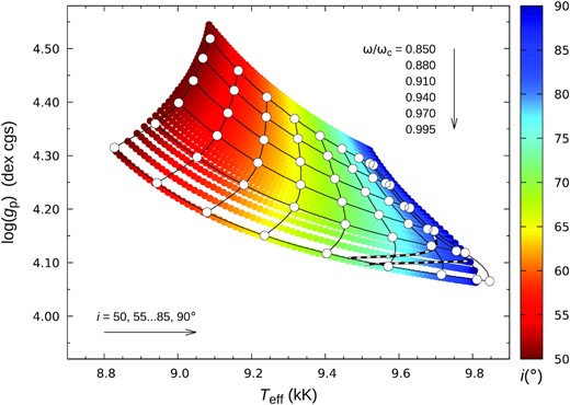
Grids of Teff, log (gp) values that reproduce the observed V, UV fluxes as functions of ωe/ωc and axial inclination, i. The base grid, colour-coded for inclination, shows results for the full set of models based on solid-body surface rotation and the Hipparcos parallax (i = 50–90○ at 0.5○ steps; ωe/ωc in the range 0.850–0.995 at steps of 0.005, with vesin i from equation B2a). The sparse grid of connected larger white dots shows a subset of corresponding results for models based on the Gaia parallax and ester differential rotation (Appendix B5), sampled as labelled in the Figure. The near-horizontal dashed lines are loci of models from each grid which have equatorial rotation periods that match the TESS photometric period.
Detailed polarization models were constructed for each parameter-grid point, as set out in Section 3.1, with results passband-integrated for comparison with the observations. The resulting χ2 map is shown in Fig. 5. Confidence intervals on this map were generated from bootstrapped data sets by evaluating best-fit inclinations for each ωe/ωc from the χ2 maps, for 1000 samplings. The 1σ ranges give the corresponding Δχ2, from which the confidence intervals may be inferred.
![Map of χ2 comparisons of observed and modelled polarizations (models based on solid-body surface rotation, the Hipparcos parallax, and [M/H] = −0.5). The dashed black line shows an analytical approximation to the minimum-χ2 locus (equation 5), with solid black lines corresponding to 1σ, 2σ, and 3σ confidence intervals on the range of acceptable models (Section 4). Dash–dot lines show the loci of solid-body surface-rotation models with equatorial rotation periods that match the TESS photometric period (upper, lower for Hipparcos, Gaia parallaxes, respectively). The solid white lines are corresponding results for ester-model differential rotation. Grey lines are for Gaia-parallax, ester-rotation models which have equatorial rotation periods differing from Pphot by +1/ −1 per cent (upper/lower lines). White dots mark four of the models listed in Table 5, with the yellow star corresponding to the adopted ‘base’ model therein.](https://oup.silverchair-cdn.com/oup/backfile/Content_public/Journal/mnras/520/1/10.1093_mnras_stad149/1/m_stad149fig5.jpeg?Expires=1750221637&Signature=NPTs23BKtmE4TfdkaroycQw3Nk2Ngc9RLRB2XQ1ZdPhwP8ykZm-9O9holV5tgG-ursYovEKdccaU-NNzAfwax74rR4GjefZzodztJgaYVM1H54k8r-Uox31pCGfTUy5BU24JY~GFXn2-KzbADXIwiQkplFFhhngafZwaQMVo4ivh7NDbV28a5gMy9RIWxDY3tBQBqrF7pYtudOpO4JA7D6YLUolBpqkl3f4czQq70eEZGk5t8h~RkIyx-jt7tOAIU43pinWQMWCnaYYuDsvu99v~K4C-i3b0C5tPIA0PBo-VIepp~pB9lGxz66M7zkBEH8RxyuK6Rrdvoqr06VD7Rw__&Key-Pair-Id=APKAIE5G5CRDK6RD3PGA)
Map of χ2 comparisons of observed and modelled polarizations (models based on solid-body surface rotation, the Hipparcos parallax, and [M/H] = −0.5). The dashed black line shows an analytical approximation to the minimum-χ2 locus (equation 5), with solid black lines corresponding to 1σ, 2σ, and 3σ confidence intervals on the range of acceptable models (Section 4). Dash–dot lines show the loci of solid-body surface-rotation models with equatorial rotation periods that match the TESS photometric period (upper, lower for Hipparcos, Gaia parallaxes, respectively). The solid white lines are corresponding results for ester-model differential rotation. Grey lines are for Gaia-parallax, ester-rotation models which have equatorial rotation periods differing from Pphot by +1/ −1 per cent (upper/lower lines). White dots mark four of the models listed in Table 5, with the yellow star corresponding to the adopted ‘base’ model therein.
Stellar parameters for initial models (solid-body surface rotation), spanning the range of allowed inclinations. For given i, the value of ωe/ωc follows from equation (5) (excepting the ‘ω2 ±’ models), and thence vesin i from equation (B2). The final three rows are the position angles of the stellar rotation axis and the interstellar polarization (each in the range 0:180○), and the magnitude of peak polarization (equation 2). The ‘ω2 +’ and ‘ω2 −’ columns correspond to changes of ±2σ in ωe/ωc at the extremes of i. The majority of the tabulated results were obtained by adopting the Hipparcos parallax, with the final two columns being for the Gaia parallax, at the extremes of allowed inclinations.
| Parameter | Unit | Hipparcos | ω2+ | ω2 − | Gaia | ||||||
|---|---|---|---|---|---|---|---|---|---|---|---|
| i | ○ | 60 | 70 | 80 | 90 | 63 | 90 | 58 | 90 | 60 | 90 |
| ωe/ωc | 0.972 | 0.953 | 0.943 | 0.998 | 0.954 | 0.999 | 0.931 | 1.000 | 0.943 | ||
| vesin i | km s−1 | 324 | 316 | 312 | 311 | 323 | 312 | 324 | 309 | 319 | 311 |
| Teff | kK | 9.02 | 9.44 | 9.63 | 9.68 | 9.14 | 9.71 | 8.98 | 9.66 | 9.02 | 9.68 |
| Tp | kK | 10.60 | 10.79 | 10.90 | 10.90 | 10.70 | 10.99 | 10.53 | 10.82 | 10.60 | 10.90 |
| Te | kK | 6.47 | 8.19 | 8.56 | 8.68 | 7.05 | 8.62 | 6.65 | 8.74 | 6.45 | 8.69 |
| Rp | R⊙ | 2.13 | 2.14 | 2.15 | 2.15 | 2.14 | 2.14 | 2.12 | 2.16 | 2.19 | 2.21 |
| Re | R⊙ | 3.14 | 2.84 | 2.76 | 2.73 | 3.09 | 2.76 | 3.10 | 2.71 | 3.23 | 2.81 |
| Prot | h | 10.20 | 10.23 | 10.58 | 10.68 | 10.33 | 10.73 | 9.86 | 10.64 | 10.66 | 10.97 |
| |$\overline{\theta }$| | mas | 0.97 | 0.91 | 0.89 | 0.89 | 0.96 | 0.89 | 0.97 | 0.88 | 0.97 | 0.89 |
| log (gp) | dex cgs | 4.17 | 4.19 | 4.18 | 4.18 | 4.16 | 4.17 | 4.19 | 4.20 | 4.14 | 4.17 |
| log (ge) | dex cgs | 2.52 | 3.48 | 3.59 | 3.64 | 2.88 | 3.57 | 2.71 | 3.70 | 2.48 | 3.63 |
| M | M⊙ | 2.42 | 2.58 | 2.55 | 2.57 | 2.40 | 2.46 | 2.55 | 2.69 | 2.41 | 2.64 |
| log (L/L⊙) | dex | 1.63 | 1.67 | 1.69 | 1.70 | 1.65 | 1.70 | 1.61 | 1.69 | 1.65 | 1.72 |
| θ* | ○ | 71.4 | 71.5 | 71.5 | 71.5 | 71.4 | 71.5 | 71.3 | 71.4 | ||
| θi | ○ | 56.8 | 55.4 | 53.7 | 53.7 | 58.1 | 54.1 | 55.2 | 51.5 | ||
| p(λmax) | ppm | 22.0 | 20.2 | 18.4 | 18.3 | 24.0 | 18.7 | 20.2 | 16.6 | ||
4.1 The rotation-period ‘problem’...
Table 3 shows that, for the initial parameter grid, the surface rotation periods, Prot, along the χ2 ‘valley’ of Fig. 5 are in the range 10.2–10.7 h (for i = 60 → 90○). These values are sufficiently close to the TESS photometric period (Pphot = 11.1 h; Section 2.2) to suggest that the photometric period may very well be the rotation period.
In part to see if the model Prot values could be straightforwardly reconciled with Pphot, we conducted parameter-sensitivity tests, and also recalculated the parameter grid with the Gaia parallax (which, being smaller, leads to slightly larger radii, hence larger values of Prot for given ve). Selected results are included in Tables 3 (Gaia parallax, columns 11, 12) and 4 (sensitivity tests).
Parameter sensitivity to fixed inputs, showing differences (model minus base) with respect to a reference model having i = 80○, ωe/ωc = 0.953, vesin i = 312.3 km s−1, [M/H] = −0.50, Hipparcos parallax (π = 39.28 mas), |$E(B-V) = 0{${_{.}^{\rm m}}}005$|, and solid-body surface rotation.
| Parameter | Base | [M/H] | π/mas | E(B − V) | UV flux | vesin i | ωe/ωc | ||||
|---|---|---|---|---|---|---|---|---|---|---|---|
| value | =0.0 | =38.23 | |$=0{${_{.}^{\rm m}}}0$| | × 1.05 | /1.05 | +5 km s−1 | −5 km s−1 | +0.01 | −0.01 | ||
| Teff | kK | 9.632 | +0.174 | +0.002 | −0.038 | +0.091 | −0.090 | −0.001 | +0.001 | +0.020 | −0.018 |
| log (gp) | dex cgs | 4.180 | +0.014 | −0.012 | +0.001 | +0.005 | −0.005 | +0.014 | −0.014 | −0.015 | +0.015 |
| Rp/R⊙ | 2.148 | −0.067 | +0.058 | −0.005 | −0.025 | +0.025 | +0.000 | −0.001 | −0.008 | +0.007 | |
| Re/R⊙ | 2.762 | −0.087 | +0.074 | −0.007 | −0.032 | +0.032 | +0.000 | −0.001 | +0.031 | −0.028 | |
| M/M⊙ | 2.547 | −0.079 | +0.069 | −0.006 | −0.029 | +0.030 | +0.083 | −0.081 | −0.107 | +0.104 | |
| log (L/L⊙) | 1.690 | +0.003 | +0.023 | −0.009 | +0.006 | −0.006 | +0.000 | +0.000 | +0.007 | −0.007 | |
| Prot | h | 10.575 | −0.330 | +0.285 | −0.025 | −0.122 | +0.125 | −0.165 | +0.170 | +0.055 | −0.049 |
The inferred effective temperature is, unsurprisingly, mildly sensitive (at the ∼100 K level) to [M/H], and to the value of the integrated UV flux, but other parameters (including Prot) appear to be quite robustly determined, with changes that are generally within the spread of values resulting from the i, ωe/ωc indeterminancy. This robustness propagates into the polarization modelling; a solar-abundance test grid (with concomitant changes in all basic parameters) gives a χ2 map that is practically indistinguishable from that shown in Fig. 5, confirming our expectation that the modelled polarization is primarily sensitive to i and to ωe/ωc, with relatively little dependence on other parameters (within reasonable bounds).
Although confirming the obvious result that smaller parallax (greater distance, hence larger radius) and smaller vesin i should push Prot to larger values, the model rotation periods in Tables 3 and 4 still all fall short of Pphot. The differences are smallest for the highest-inclination, Gaia-parallax models, with the extreme i = 90○ model in Table 3 requiring a reduction of only ∼5 km s−1 in vesin i to force agreement. However, Fig. B1(f) indicates that even as small a change as this is barely compatible with the line-profile analysis (for a continuum placement chosen to give consistency with solid-body surface rotation, which already results in lower vesin i values than would otherwise be found; Fig. B3).
We conclude that the combined hypotheses of both (i) solid-body surface rotation and (ii) Pphot = Prot, while not completely ruled out, are at best only marginally consistent with the data.
4.2 ...and some possible resolutions
There are several possible circumstances that could address this modest discrepancy between Prot and Pphot. For example, reducing the Gaia parallax by ∼2σ would increase the distance, model radius, and hence Prot, by a further ∼2 per cent (although the parallax would then be ∼11σ from the Hipparcos value). Such ‘fine tuning’ cannot be excluded; nevertheless, we should also not discount the possibility that Pphot need not necessarily be identical to the solid-body rotation period.
We note, for example, that both g- and r-mode pulsation periods can be in the same range as the rotation period. The attraction of pulsation as the origin of photometric variability is that it does not require time-variable magnetic fields to be invoked as a mechanism to generate rotational modulation through starspots (in a broad sense). Where magnetic fields have been directly detected in OBA stars (which are thought to have primarily radiative envelopes), they appear to be fossil remnants, an interpretation consistent with associated highly reproducible, strictly periodic photometric and spectroscopic variability (e.g. Hubrig & Schöller 2021). This behaviour contrasts with much of the low-amplitude variability revealed by space photometry and widely attributed to rotational modulation (e.g. Balona & Abedigamba 2016).
Saio et al. (2018) found a low-frequency ‘hump’ in time-series power spectra at frequencies just below the rotation frequency, resulting from r-mode pulsation with azimuthal wavenumber |m| = 1. Subsequently, Lee & Saio (2020) and Lee (2021, 2022) have shown that overstable convective modes in the core of an early-type star can couple with g modes in the radiative envelope, provided the core rotates slightly faster than the envelope. These modes are therefore candidates for the processes underlying the photometric variability.
However, the r-mode modelling suggests a more complex frequency spectrum than is exhibited by ζ Aql A, while the periods driven by overstable convective modes should necessarily be shorter than the surface rotation periods (whereas, we find to the contrary, that Pphot ≳ Prot). While pulsational variability close to the rotation frequency remains a possibility, arguments in favour of that hypothesis do not appear compelling at present.
4.3 Differential rotation?
If, instead, the photometric variability is attributed to rotational modulation of surface-brightness inhomogeneities then differential surface rotation offers a straightforward solution to the discrepancy between the modelled (equatorial) rotation period, Prot(e), and Pphot: spots could simply be at latitudes rotating with a different angular speed.
As described in Appendix B2, an ad hoc parametrization of differential rotation was considered as part of our initial examination of rotational velocities. That analysis of the line-profile shape found no direct evidence for substantial differential rotation. However, a purely empirical approach cannot rule out lower-level differential rotation, and necessarily introduces an arbitrary element (i.e., an ad hoc characterization of the dependence of ω on colatitude θ).
For a second phase of the analysis, we therefore pursued a direct physical approach, using surface-rotation profiles, ω(θ), generated from ester 2D stellar-structure models, as elaborated in Appendix B5 (and illustrated in Fig. B2).
We first repeated the exercise of establishing the relationship between vesin i and ωe/ωc for these differentially-rotating models (cf. Appendices B4,B5), then generated new parameter grids (for both Hipparcos and Gaia parallaxes). Selected results are incorporated into Figs 4 and 5. Fig. 5 shows that only the combination of Gaia parallax and ester rotation profiles gives agreement between Prot(e) and Pphot at i, ωe/ωc values that are consistent with the polarimetry, without requiring any fine tuning.
This result arises because ester-type differential rotation has greatest angular velocity at temperate latitudes (Fig. B2), leading to projected equatorial rotation velocities that are generally ∼1–2 per cent smaller than rigid-rotator results (Appendix B5). The relationships between vesin i and ωe/ωc are essentially independent of parallax, but with lower ve values favoured by lower ωe/ωc and by higher inclinations. The combination of these effects, along with their non-linear dependences on ωe/ωc, means that, within the χ2 valley of Fig. 5, Prot(e) matches Pphot only for Gaia+ester models, at high inclinations (i ≳ 80○, such that ve ≃ vesin i) for the ωe/ωc values indicated by the photopolarimetry.
Given the sensitivity of Prot(e) to rather small changes in vesin i, this is clearly not a unique result (nor a strong validation) of the ester rotation profile. For example, an arbitrary surface-rotation law of the form of equation B1, with α ∼ −0.03, would give a similar outcome. Nevertheless, the success of the (almost) ‘no free parameters’ ester models in bringing about agreement between Prot(e) and Pphot is encouraging and suggestive.
A further caveat is that Fig. 5 is not fully self-consistent, as the various Pphot = Prot(e) lines are calculated under slightly different sets of assumptions, while the χ2 map is specifically for solid-body surface rotation and the Hipparcos parallax. We have not addressed this minor inconsistency, for several reasons:
We consider the existing calculations already to be sufficient to demonstrate that the modelled Prot(e) and observed Pphot can readily be reconciled; while other stellar parameters are insensitive to details of the rotation profile and parallax.
We know the χ2 map is very insensitive to most input parameters (including small changes in parallax), excepting the i, ωe/ωc pair. While any sensitivity to differential surface rotation is less clear, it is unlikely to be large, given the small departures from solid-body rotation implied by the ester profiles (and the empirical limits on strongly differential rotation).
If the photometric variability does arise from starspots, we do not know their latitude(s). Although we have focused on reconciling the equatorial rotation period of the models with Pphot, the spot rotation periods could easily be 1–2 per cent different (in either direction) in the presence of differential surface rotation. As shown in Fig. 5, such small differences can have a relatively large effect on the location of the Prot(e) locus in the i, ωe/ωc plane, which is likely to dominate the uncertainties.
5 DISCUSSION
Selected numerical results for the Gaia+ester parameter grid are given in Table 5 (other parameter grids give results intermediate between those in Tables 3 and 5). We take the ‘base’ model listed there, for which Prot(e) = Pphot, as our adopted specific solution. If starspots do give rise to the photometric variability, then the combination of high axial inclination and ∼continuous variation implies that they must have an extensive distribution in longitude.
| Parameter | Unit | Base | Variants | |||
|---|---|---|---|---|---|---|
| i | ○ | 84.9 | 82.4 | 77.9 | 90.0 | 90.0 |
| ωe/ωc | 0.946 | 0.931 | 0.968 | 0.957 | 0.925 | |
| vesin i | km s−1 | 306 | 304 | 311 | 308 | 303 |
| Teff | kK | 9.693 | 9.638 | 9.645 | 9.741 | 9.661 |
| Tp | kK | 10.952 | 10.817 | 11.020 | 11.063 | 10.814 |
| Te | kK | 8.680 | 8.733 | 8.434 | 8.634 | 8.790 |
| Rp | R⊙ | 2.21 | 2.22 | 2.19 | 2.20 | 2.22 |
| Re | R⊙ | 2.82 | 2.78 | 2.89 | 2.84 | 2.77 |
| Prot(e) | h | 11.12 | 11.00 | 11.00 | 11.20 | 11.07 |
| |$\overline{\theta }$| | mas | 0.89 | 0.88 | 0.90 | 0.89 | 0.88 |
| log (gp) | dex cgs | 4.15 | 4.18 | 4.14 | 4.14 | 4.18 |
| log (ge) | dex cgs | 3.60 | 3.68 | 3.47 | 3.53 | 3.70 |
| M | M⊙ | 2.53 | 2.71 | 2.42 | 2.41 | 2.73 |
| log (L/L⊙) | dex | 1.72 | 1.71 | 1.73 | 1.74 | 1.71 |
The line-profile modelling for the adopted solution is shown in Fig. 6, the predicted and observed polarizations in Fig. 7, and the flux distributions in Fig. 8. All these comparisons show satisfactory agreement between models and observations.
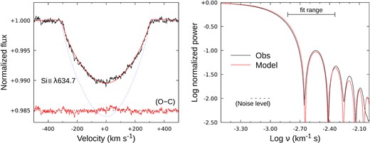
Left: observed and modelled Si ii profiles for the base model of Table 5 (vesin i = 306 km s−1; ester rotation, Gaia parallax). The model line depth has been scaled by 0.95× to facilitate comparison of line shapes; the dotted blue line shows an otherwise identical model (including the ad hoc scaling) for solar abundances. Right: the normalized Fourier transforms, showing the frequency range over which the observed and modelled transforms were compared (Section B2); the white-noise power level is indicated.
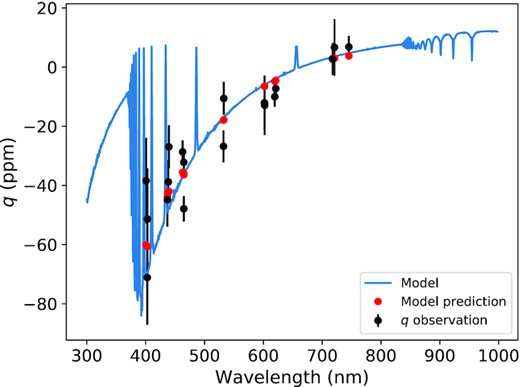
Comparison of observed and modelled polarizations. Red dots are passband-integrated model results. The ‘observed’ values have been corrected for foreground interstellar polarization, and rotated so that the polarization is entirely in q. The model is for solid-body surface rotation at i = 85○, ωe/ωc = 0.95.
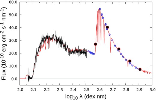
Comparison of measured and modelled fluxes. Observed IUE and UBVRI fluxes are shown in black. Optical spectrophotometry from Breger (1976) and Adelman, Pyper & White (1980), normalized at 500 nm, is shown as small blue dots (but was not used in the modelling). The ‘base’ model of Table 5, reddened with |$E(B-V) = 0{${_{.}^{\rm m}}}005$|, is shown in red.
The mean angular diameters predicted by the tabulated models are in excellent accord with the interferometric value given by Boyajian et al. (2012; 0.895 ± 0.017 mas), but are inconsistent with the interim analysis reported by Peterson et al. (2006; cf. Table 1); their values of i = 90○, ωe/ωc = 0.99, θ* = 45○ are also at odds with the photopolarimetric results (Table 3).5
5.1 Comparison with evolutionary models
We compare our empirical results with models of the evolution of rotating stars from Georgy et al. (2013) in Fig. 9.6 Their grids are for a range of ZAMS rotation rates, ωe/ωc(0), and include metallicities representative of solar and LMC abundances (Z = 0.006, corresponding to [M/H] ≃ −0.4). All our empirically determined masses fall within the range |$M=2.53^{+0.20}_{-0.13}\,\mbox{M}_{\odot }$|, in excellent agreement with the evolutionary mass for the solar-abundance tracks. The LMC-abundance tracks suggest evolutionary masses ∼0.3 M⊙ lower, barely consistent with empirical values.
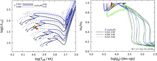
Left: Hertzsprung–Russell diagram. Evolutionary tracks are from Georgy et al. (2013) for the indicated ZAMS masses (in solar units), metallicities Z, and initial (ZAMS) ωe/ωc values. Yellow stars show all the solutions from Table 5, although they are almost inseparable in this plot. Red dots show results from Table 3; additional solutions from the sensitivity tests (Table 4) all fall under the yellow stars. Right: evolution of model ωe/ωc values. Overall, evolution is from higher to lower gravities; the ∼horizontal regions at log (gp) ≃ 4 correspond to the main-sequence phase.
Main-sequence A-type stars show a range of surface-abundance anomalies, usually involving selective metal enhancements (the Am, Ap, and HgMn stars); only stars in the λ Boo class are noted for their metal depletions. This group is also characterized by relatively rapid rotation. While ζ Aql is not a classic λ Boo star in terms of its spectral morphology (Gray, personal communication), its subsolar metallicity may arise through a similar mechanism, generally thought to involve photospheric accretion of depleted gas (e.g. Venn & Lambert 1990; Jermyn & Kama 2018). In that case, we would expect solar abundances to be more relevant to its evolution, as found in these comparisons
At these masses, the evolutionary tracks are not strongly sensitive to the precise value of ωe/ωc(0), although a high value is, of course, required for ζ Aql A. A ZAMS value close to ∼0.95 is consistent with observations (Fig. 9, right-hand panel).
6 SUMMARY AND CONCLUSIONS
We have presented new, very precise photopolarimetry of ζ Aql (Table 2). Modelling those observations, together with supplementary analyses of the flux distribution and rotational velocity, allows us to determine the locus of allowed combinations of i and ωe/ωc (Fig. 5). The polarimetry alone cannot break the degeneracy between these two parameters, but limits their values to i ≳ 60○, ωe/ωc ≳ 0.93.
Periodic photometric variability, demonstrated here for the first time (from TESS observations), provides additional constraints under the plausible assumption that the newly established photometric period, Pphot = 11.12 h, can be identified with the rotation period. The rotation periods of models based on rigid-body surface rotation are only marginally consistent with Pphot, requiring extreme values and fine tuning of parameters to push ve and/or the parallax to appropriately low values. However, model equatorial rotation periods are found to be in good agreement with Pphot for the combination of Gaia parallax and the differential surface rotation predicted by ester models.
The inferred physical parameters of ζ Aql A are quite insensitive to these issues, as demonstrated by the small range of solutions listed in Tables 3–5; our adopted specific characterization is given in column 3 of Table 5. Taking the full ranges of parameter values in that Table as a reasonably conservative estimate of the 1σ uncertainties, we find |$M = 2.53\pm 0.16\, \mbox{M}_{\odot }$|, log (L/L⊙) = 1.72± 0.02, |$R_{\rm p}= 2.21\pm 0.02\, \mbox{R}_{\odot }$|, Teff = 9693 ± 50 K, |$i = 85{^{+5}_{-7}}^\circ$|, and ωe/ωc = 0.95 ± 0.02.
Comparison of our results with grids of single-star evolution calculations shows excellent agreement for solar-abundance models, but poorer agreement with models at lower metallicities that approximately match the depleted surface abundances. This suggests that the observed photospheric depletions may not be global, but instead confined only to the surface layers.
ACKNOWLEDGEMENTS
This paper is based in large part on data obtained with the Anglo-Australian Telescope at Siding Spring Observatory; we acknowledge the traditional owners of the land on which the AAT stands, the Gamilaraay people, and we pay our respects to elders past and present. We made use of the Washington Double Star Catalog, maintained at the U.S. Naval Observatory, as well as observations made with the International Ultraviolet Explorer and TESS satellites, obtained from the MAST data archive at the Space Telescope Science Institute, which is operated by the Association of Universities for Research in Astronomy, Inc., under NASA contract NAS 5-26555. Funding for the TESS mission is provided by the NASA Explorer Program. CFHT data were accessed by using the facilities of the Canadian Astronomy Data Centre, operated by the National Research Council of Canada with the support of the Canadian Space Agency. We also benefitted from NASA’s Astrophysics Data System bibliographic service, and the SIMBAD data base, operated at CDS, Strasbourg, France. We thank Nicholas Borsato, Dag Evensberget, Behrooz Karamiqucham, Jonathan Marshall, and Jinglin Zhao for contributions to observing runs, our anonymous referee for useful remarks, and Conny Aerts, Derek Buzasi, Richard Gray, and Michel Rieutord for helpful correspondence. DVC thanks the Friends of MIRA for their support.
DATA AVAILABILITY
The new polarization data used for this project are listed in Table 2. All other data are from publicly accessible archives.
Footnotes
Wallenquist used a wedge photometer; therefore, although the observation was visual, it is nevertheless a measurement, not merely an estimate.
The similarity of the implied ΔK, 4|${_{.}^{\rm m}}$|4, to that of the B component must be coincidental; the field of view of the instrument used to detect the excess is only |$0{_{.}^{\prime\prime}} 8$| (fwhm). However, Absil et al.’s discussion of the infrared photometric results will be compromised by their neglect of the companion star’s flux contribution.
We define the (global) effective temperature for a gravity-darkened star through the stellar luminosity,
where |$T_{\rm eff}^{\ell }$| is the local (latitude-dependent) effective temperature and the integrals are over surface area. The ratio of polar to effective temperatures is solely a function of ωe/ωc (for given gravity-darkening and surface-rotation prescriptions); in the case of ω-model gravity darkening and rigid-body surface rotation, Tp/Teff = 1.09 → 1.16 for ωe/ωc = 0.85 → 0.99.
The Tp, ωe/ωc, i triplet reported by Peterson et al. (2006) requires θp≃ 0.75 mas (|$\overline{\theta }$| ≃ 0.88 mas) in order to reproduce the observed V magnitude. The disagreement with their published value, θp= 0.815 ± 0.005 mas, suggests that there may be typographical errors in their tabulated numbers.
It is an early version of this comparison that underpinned the choice of parameters adopted for the ester modelling described in Section B5.
We observe that this formulation, widely used in the cool-star community, is entirely ad hoc; its form can be traced back to Carrington (1863, p. 223, albeit with an exponent of |$7/_{4}$|).
‘Normalized’ here means dividing the power by the lowest-frequency value, which accounts for any small residual differences between observed and modelled line strengths.
In this particular case, the line equivalent width is roughly constant over the range of relevant temperatures, and it is the temperature dependence of the continuum that is the dominant effect. The ‘visible’ parts of the star still provide sufficient information to constrain vesin i and α, for given ωe/ωc.
REFERENCES
APPENDIX A: SUMMARY OF OBSERVING RUNS
Technical details of the observing runs leading to the results given in Table 2 are summarized in Table A1. HIPPI and HIPPI-2 are dual-beam photopolarimeters that use ferroelectric liquid crystals (FLCs) for primary modulation at 500 Hz, in order to overcome seeing noise and thereby to achieve high precision. The FLC used for all HIPPI/-2 observations of ζ Aql was manufactured by Boulder Nonlinear Systems; the performance of this unit has evolved over time, an issue addressed by the reduction pipeline used to process all the data from both instruments (Bailey et al. 2020a).
We made use of two types of Hamamatsu photomultiplier tube (PMT) as detectors; the blue-sensitive H10720-210, which we denote ‘B’, and red-sensitive H10720-20, ‘R’. Six broadband filters were employed: custom-built 425-nm and 500-nm ‘short-pass’ and 650-nm ‘long-pass’ filters (425SP, 500SP, and 650LP, respectively; Bailey et al. 2020a), SDSS g′ and r′, and Johnson V. The r′ filter was paired with both the R and B detectors; the 650LP filter only with R; and the remainder only with B.
Telescope optics introduce a small wavelength-dependent polarization, which was removed by reference to observations of low-polarization standard stars (cf. Table A1).
Summary of observing runs.
| Telescope and instrument set-upa | Tel. calibrationb | ||||||||||
|---|---|---|---|---|---|---|---|---|---|---|---|
| Run ID | Date rangec | Instr. | Tel.d | f/ | Ap. | Mod. | Filter | Det.e | n | qTP | uTP |
| (UT) | (″) | (ppm) | (ppm) | ||||||||
| 2005_04 | 04/25–05/08 | PlanetPol | WHT | 11 | 5.2 | PEM | BRB | APD | 1 | (Note f) | |
| 2015_10 | 10/14–11/02 | HIPPI | AAT | 8 | 6.6 | BNS-E1 | g′ | B | 1 | −50.4 ± 1.1 | −0.2 ± 1.1 |
| 2017_08 | 08/12–07/04 | HIPPI | AAT | 8 | 6.6 | BNS-E2 | 425SP | B | 1 | −7.3 ± 3.6 | 8.5 ± 3.6 |
| 500SP | B | 1 | −10.0 ± 1.7 | −0.4 ± 1.6 | |||||||
| g′ | B | 1 | −9.1 ± 1.5 | −2.6 ± 1.4 | |||||||
| r′ | R | 1 | −10.4 ± 1.3 | −7.0 ± 1.3 | |||||||
| 650LP | R | 1 | −8.2 ± 2.3 | −5.1 ± 2.4 | |||||||
| 2018_07 | 07/15–07/23 | HIPPI-2 | AAT | 16g | 11.9 | BNS-E4 | 425SP | B | 2 | −5.6 ± 6.4 | 19.8 ± 6.3 |
| 500SP | B | 2 | 1.9 ± 1.4 | 18.4 ± 1.4 | |||||||
| g′ | B | 1 | −12.8 ± 1.1 | 4.1 ± 1.0 | |||||||
| V | B | 2 | −20.3 ± 1.5 | 2.3 ± 1.5 | |||||||
| r′ | B | 1 | −10.4 ± 2.2 | 3.7 ± 2.2 | |||||||
| r′ | R | 1 | −12.7 ± 1.2 | 0.4 ± 1.2 | |||||||
| 650LP | R | 1 | −6.6 ± 1.9 | 4.0 ± 1.9 | |||||||
aInstr. is the instrument; ‘Tel.’, ‘f/’ the telescope and its f-ratio; ‘Ap.’ the angular diameter, on the sky, of the photometer entrance aperture; ‘Mod.’ the modulator; ‘Det.’ the detector; and n the number of independent observations. Further details, including transmission curves for all components and characterizations of each modulator at the relevant epochs, can be found in Hough et al. (2006) and Bailey et al. (2020a). bThe observations used to determine the telescope-induced polarization, TP, and the high-polarization standards observed to calibrate position angle, are described by Marshall et al. (2016, run 2015_10), Cotton et al. (2019, run 2017_08), and Bailey et al. (2020a, run 2018_07). cDates given are inclusive of ζ-Aql and standard-star observations. dWHT, 4.2-m William Herschel Telescope (altazimuth mount); AAT, 3.9-m Anglo-Australian Telescope (equatorial mount). eB, R indicate blue- and red-sensitive photomultiplier tubes, respectively (Section 2.1); APD indicates PlanetPol’s Avalanche Photo-Diodes, which resulted in a broad red bandpass (BRB) extending beyond ∼1 |$\mu$|m. fThe telescope-polarization function for this altazimuth telescope is discussed by Bailey et al. (2010). gFocal ratio increased by using a 2× negative achromatic lens.
APPENDIX B: ROTATIONAL VELOCITY
The equatorial rotation velocity provides an important constraint on the stellar mass. A summary of published estimates of vesin i for ζ Aql A is given in Table B1; Abt & Morrell (1995) provide the only primary measurement on the Slettebak et al. (1975) system that we have been able to locate. They note the absence of reliable fast-rotating calibrators in their data set, and mark their measurement as uncertain. We therefore undertook a new analysis in order to determine a modern precise value for vesin i, using the Fourier-transform method (e.g. Carroll 1933; Smith & Gray 1976).
Literature vesin i values.
| Value (km s−1) | Source | Notes |
|---|---|---|
| Primary sources: | ||
| 175 | Westgate (1933) | [1] |
| 365 | Slettebak (1954) | |
| 350 | Slettebak (1966) | [2] |
| 305 | Palmer et al. (1968) | |
| 295: | Abt & Morrell (1995) | |
| Secondary sources: | ||
| 335 | Boyarchuk & Kopylov (1964) | [3] |
| 345 | Uesugi & Fukuda (1982) | [4] |
| 317 | Royer et al. (2002) | [5] |
Note.[1] ζ Aql is identified by Westgate only as Boss 4858; though unattributed, this refers to [Lewis] Boss (1910), not his son’s later, better-known ‘General Catalogue’ ([Benjamin] Boss 1937). [2] Most tabulated values given to the nearest 50 km s−1. [3] Appears to be a straight, albeit proleptic, average of Slettebak (1954) and Palmer et al. (1968) values. [4] Weighted average of rescaled earlier results. [5] Rescaling of Abt & Morrell (1995) result. Uncertainty of ±38 km s−1 quoted by Cochetti et al. (2020).
B1 Data
A search of online archives showed that observations obtained with the ESPaDOnS echelle spectropolarimeter at the Canada–France–Hawaii Telescope (CFHT) are of particularly good quality, and numerous. After rejecting a handful of relatively low-quality exposures, we corrected relevant sections of each of the remaining sixty-three spectra for weak telluric absorption (dividing individual spectra by a scaled telluric template constructed from the data merged in topocentric velocity space), then merged them (after correcting to heliocentric velocities). The resulting noise-weighted mean spectrum has a continuum signal:noise ratio of ≳3000 at ∼635 nm (as measured from residuals to low-order polynomial fits), at a resolving power of R ≃ 65 000. We identified no obvious line-profile or radial-velocity variability in these data (Section 2.3.5).
B2 Modelling: ad hoc characterization of differential rotation
Latitudinal differential rotation introduces changes to line-profile shapes, principally by modifying the Doppler redistribution of absorption arising at temperate latitudes (for given ve and sin i; changes in gravity darkening introduce further, but secondary, effects). This in turn affects the Fourier transform of the profiles – notably, the separation of the first and second minima (e.g. Reiners, Schmitt & Kürster 2001; Reiners & Schmitt 2002).
We computed synthetic spectra (incorporating full Roche-model rotational effects) over a space intended to cover the likely range of parameter values at suitable sampling densities:
vesin i in the range 270:330 km s−1, at steps of 2 km s−1;
sin i, 0.72:1.00 @ 0.02;
ωe/ωc, 0.85:0.99 @ 0.01; and
α, −0.24:+0.24 @ 0.03.
First results for regions around Ca ii K, Mg ii 448.1 nm, and Si ii 634.7 nm showed that significantly subsolar metallicity is required to match observed line strengths, in accord with reports by Gray et al. (2003) and Wu et al. (2011); we obtained reasonable agreement for [M/H] ≃ −0.5, and adopted that value. We then focused on the |$\rm{Si {\small II}}$| λ634.7 line profile for analysis, as it is one of the very few features not to show obvious blending in the spectra employed. (Although least-squares deconvolution is ostensibly capable of addressing the blending issue, and of improving the overall signal:noise, its underpinning principles do not hold when gravity darkening is significant, as is the case here. Moreover, systematics, rather than stochastic noise, prove to dominate uncertainties in the conclusions.)
For each model spectrum, the required values for Teff and polar radius (a surrogate for polar gravity in these circumstances) were those that reproduce the observed V, UV fluxes, for the matching vesin i, ωe/ωc, and inclination values, as discussed in Section 3.2, but for rigid rotation (regardless of the spectrum-synthesis value of α). This approximation, adopted for computational expedience, is of no consequence for the vesin i analysis (as is also true for the adopted metallicity).
The comparison between observed and modelled λ634.7 nm profiles was conducted in Fourier space, using the rms differences between normalized transforms8 as a test statistic. Precise numerical results depend on the exact frequency (inverse velocity) interval chosen for the comparison, but our general conclusions are insensitive to this, for any reasonable values. We used the range (1.5–4.5) × 10−3 km−1 s, which encompasses the first two minima in the transform (Fig 6); including the third minimum does not materially change any conclusions, but starts to run into the noise. We found no evidence for any additional broadening processes (‘macroturbulence’) beyond the basic physical mechanisms integral to the modelling.
B3 Ad hoc characterization: an empirical limit on differential rotation
Some results of the initial analysis are summarized in Fig. B1. The basic empirical test for differential rotation is embodied in panel (a), where the minimum rms FT O−C for any (sin i, ωe/ωc) combination is shown as a function of vesin i and α. This figure hints at possibly antisolar differential rotation (i.e. negative α), which would contrast with the handful of positive-α A-star detections reported in the literature (Reiners & Royer 2004; Ammler-von Eiff & Reiners 2012).
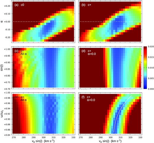
Heatmaps summarizing comparisons of observed and model Fourier transforms for the |$\rm{Si {\small II}}$| λ634.7 line; the test statistic is the rms difference between observed and modelled normalized Fourier transforms (so smaller values mean better matches), taking the minimum values over marginal variables. Panels (a) and (b), marginalized over ωe/ωc and i, represent results for two slightly different rectifications of the observed profile, ‘c0’ and ‘c+’, described in Section B3. Panels (c) and (e) are marginalized over all values of α, while (d) and (f) are for solid-body surface rotation (α ≡ 0; panels (c)–(f) are all based on the c+ rectification). The solid line in panel (f) is equation (B2).
However, we find that quite small revisions to the adopted continuum normalization can introduce significant changes to the transform (cf. Dravins, Lindegren & Torkelsson 1990). We label our initial, ‘by eye’, continuum as ‘c0’ in the accompanying figures. Modifying the observed profile by division [resp., multiplication] with a cosine bell of half-width 320 km s−1 and peak amplitude 0.1 per cent of this initial continuum gives a slightly deeper [shallower] line of slightly different shape arising from the slightly higher [lower] continuum, labelled c+ [c−]. The c+ continuum leads to the results shown in Fig. B1(b), which are entirely consistent with solid-body surface rotation.
Continuum uncertainties in the rectified observations are certainly possible at this level (if only because of unrecognized weak line blends). Furthermore, although the comparison model spectra can be rectified simply by division with the corresponding model continuum, in practice this does not lead to a result well suited to comparison to observations. A degree of subjectivity therefore also enters in rectifying the models (even though this was done in an automated procedure), accommodating further potential uncertainty. We conclude that a conservative interpretation of our results is that the initial line-profile analysis alone does not provide any compelling direct evidence for differential rotation in ζ Aql A, and constrains |α| to ≲ 0.05.
B4 Ad hoc characterization: ωe/ωc dependence
Fig. B1 also illustrates the sensitivity of vesin i to other parameters of interest. The line profile offers no useful diagnostic potential for axial inclination, but there is a clear dependence of vesin i on ωe/ωc (at any fixed α; e.g. panel f). This has a straightforward interpretation: as a consequence of gravity darkening, the high-velocity equatorial belt becomes less evident in the spectrum at high ωe/ωc, requiring an increase in vesin i in order to fill in the extreme wings of the line profile (cf. Townsend, Owocki & Howarth 2004).9
(in km s−1), where ϖ = ωe/ωc − 0.9, and the (a), (b) numerical values are from otherwise identical analyses based on Hipparcos and Gaia parallaxes, respectively (and confirm the expectation of negligible sensitivity of vesin i to distance). Equation (B2a) is shown as a white line in Fig. B1(f), and represents our adopted characterization of vesin i as a function of ωe/ωc for these α ≡ 0 models (valid over the range 0.85 ≤ ωe/ωc ≲ 0.99).
B5 ESTER modelling
As discussed in Section 4.1, an initial analysis based on assumed solid-body surface rotation and the Hipparcos parallax was challenged by disparities between rotation periods implied by the models and the TESS photometric period. We therefore examined the question of differential rotational further, under the constraint of theoretical models of differential surface rotation, rather than an arbitrary ad hoc formulation. To this end, we computed a series of structure models using the ester code10 (Espinosa Lara & Rieutord 2013; Rieutord, Espinosa Lara & Putigny 2016). Ester computes the stellar structure self-consistently with the radial and latitudinal differential rotation and the meridional circulation resulting from driving by the baroclinic torque (at solar abundance).
Initial parameter modelling indicated M ≃ 2.5 M⊙, Xc ≃ 0.7, ωk ≃ 0.8; ester surface-rotation results for this parameter set are shown in Fig. B2 (and were used for most of our subsequent modelling). The sensitivity to parameter variations from this baseline set is also illustrated. Even at rather rapid rotation, only quite modest departures from solid-body surface rotation are predicted, and they are insensitive to precise values of the free parameters (within the range of uncertainty of our results).
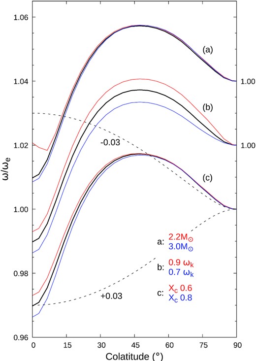
Differential surface rotation predicted from ester 2-D stellar-structure models. The reference model in each group (shown in black) is for M = 2.5 M⊙, Xc = 0.7, ωe = 0.8ωk, with the sensitivity to these parameters illustrated by results for other values, as labelled. The dashed lines show the simple ad hoc differential-rotation characterization of equation (B1), for the labelled values of the α parameter.
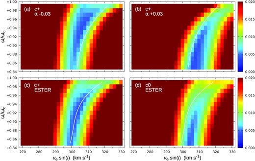
The sensitivity of inferred vesin i to assumptions in respect of differential surface rotation and rectification. Panels (a) and (b) are results for two different values of α, assuming the ad hoc characterization of equation (B1); for reference, the solid line is equation (B2a), the fit to the α = 0.0 (solid-body surface rotation) results shown in Fig. B1(f). Panels (c) and (d) show results for the reference-model ester rotation profile (Fig. B2), and two different rectifications discussed in Section B3.
