


ABSTRACT
Black hole X-ray binaries display significant stochastic variability on short time-scales (0.01–100 s), with a complex pattern of lags in correlated variability seen in different energy bands. This behaviour is generally interpreted in a model where slow fluctuations stirred up at large radii propagate down through the accretion flow, modulating faster fluctuations generated at smaller radii. Coupling this scenario with radially stratified emission opens the way to measure the propagation time-scale from data, allowing direct tests of the accretion flow structure. We previously developed a model based on this picture and showed that it could fit the Neutron star Interior Composition Explorer (NICER; 0.5–10 keV) data from the brightest recent black hole transient, MAXI J1820+070. However, here we show it fails when extrapolated to higher energy variability data from the Insight-Hard X-ray Modulation Telescope(HXMT). We extend our model so that the spectrum emitted at each radius changes shape in response to fluctuations (pivoting) rather than just changing normalization. This gives the strong suppression of fractional variability as a function of energy seen in the data. The derived propagation time-scale is slower than predicted by a magnetically arrested disc (MAD), despite this system showing a strong jet. Our new model jointly fits the spectrum and variability up to 50 keV, though still cannot match all the data above this. Nonetheless, the good fit from 3 to 40 keV means the quasi-periodic oscillation (QPO) can most easily be explained as an extrinsic modulation of the flow, such as produced in the Lense–Thirring precession, rather than arising in an additional spectral-timing component such as the jet.
1 INTRODUCTION
The nature and geometry of the X-ray emission region in black hole binaries are still controversial, especially in the low/hard state, where most of the power is emitted in a spectrum quite unlike a standard disc (Shakura & Sunyaev 1973). Spectral fitting alone is degenerate, with proposed geometries being a compact source on the spin axis (lamppost), extended emission along the jet direction (jet corona), extended coronal emission on top of an underlying accretion disc (sandwich), and extended coronal emission that replaces the accretion disc (truncated disc/hot inner flow; see e.g. Poutanen, Veledina & Zdziarski 2018). The truncated disc/hot inner flow model has the advantage that it gives a framework to explain the evolution of the spectrum and its fast variability properties together (Done, Gierliński & Kubota 2007), although there are persistent questions over the extent of disc truncation from modelling the reflected emission and its associated iron line (e.g. Buisson et al. 2019; but see Zdziarski et al. 2021a). Another way to track the extent of the disc is the quasi-thermal emission arising from the same X-ray irradiation of the disc, which gives rise to the iron line and reflected emission (De Marco et al. 2015; Wang et al. 2022). Photons that are not reflected are reprocessed in the disc, producing a thermal reverberation signal. This gives a soft lag, where variations of soft photons follow those of hard photons with a light travel time delay. Reverberation size scales do indeed point to a truncated disc, with a truncation radius that decreases as the source spectrum softens (De Marco et al. 2021). Perhaps the most compelling evidence for a truncated disc is the new polarization results for the low/hard state of Cyg X-1. These rule out the X-ray emission region being aligned with the jet and, instead, require it to be aligned with the accretion flow (Krawczynski et al. 2022). Truncated disc/hot inner flow models are thus strongly favoured, motivating our work in exploring how we can derive the physical properties of the hot flow.
The fast variability (0.01–100 s) gives independent constraints on the accretion flow. It shows many complex properties that change as a function of energy and variability time-scale (see e.g. the review by Uttley et al. 2014). The most promising framework in which to explain these is with propagating fluctuations (Lyubarskii 1997; Kotov, Churazov & Gilfanov 2001). The idea is that variability is generated in the accretion flow (e.g. by the turbulent dynamo magnetorotational instability – MRI; Balbus & Hawley 1991), with a characteristic time-scale that is shorter at smaller radii. Fluctuations generated at any radius in the hot flow propagate down so that slower fluctuations stirred up at larger radii propagate down to modulate the faster fluctuations produced at smaller radii. This produces correlated but lagged multi-time-scale variability in the entire hot flow (Lyubarskii 1997; Kotov et al. 2001). These lags can be seen directly in the data if the flow produces different spectra at different radii, with the observed ‘hard lags’ (fluctuations at 10–20 keV lagging behind the same fluctuation at 2–3 keV; Miyamoto et al. 1988; Nowak, Wilms & Dove 1999) requiring that smaller radii have harder spectra, which seems physically intuitive. Numerical models combining the propagating fluctuations process with a spectrally inhomogeneous hot flow have shown general agreement with the variability properties observed by the Rossi X-ray Timing Explorer (RXTE) in the 3–30 keV bandpass (Arévalo & Uttley 2006; Ingram & Done 2011, 2012).
However, accurately reproducing all the observed timing properties with the propagating fluctuations model turned out to be more difficult than expected in these first quantitative models, which considered only the variability in the hot flow. One approach is simply to bypass this complexity and use phenomenological models of the intrinsic variability and its lags. This is especially useful if the goal is simply to measure reverberation lags as in the reltranscode (Ingram et al. 2019). However, our goal is instead to make a physical model of the hot flow, self-consistently producing its spectrum and variability. Such models can then be used to measure physical properties, e.g. the propagation speed, which constrains the nature and geometry of the hot flow. Hence we extend the hot flow propagating fluctuation models to get a better match to the data. There are many potential ways to do this, but the goal is to identify the physical processes that make the most impact on the observed data.
One difficulty with models of propagating fluctuations through the hot flow is that this typically gives rise to a single-peaked power spectrum (Arévalo & Uttley 2006; Ingram & Done 2011, 2012), whereas the observed power spectra are often double peaked (Belloni, Psaltis & van der Klis 2002; Pottschmidt et al. 2003; Axelsson, Borgonovo & Larsson 2005; Grinberg et al. 2014). It is possible to change the time-scales and amplitude of variability with radius in the hot flow to match the data, but it seems fine-tuned (Mahmoud & Done 2018a,b). Another issue is that the observed power spectra often span a very broad range in frequencies, which is difficult to quantitatively match by the fairly small range of radii spanned by the hot flow without going to extreme parameters (Ingram & Done 2011, 2012; Mahmoud & Done 2018a,b).
A key to matching both the power spectral shape and width was the recognition that the disc generates considerable variability in the low/hard state, in addition to that expected from the hot flow (Wilkinson & Uttley 2009; Uttley et al. 2011). While the disc does not contribute to the RXTE bandpass (>3 keV) in the low/hard state, its variability will propagate down into the hot flow, so it will strongly affect the variability properties. Rapisarda et al. (2016) proposed that the inner edge of the disc had a much longer variability time-scale than the outer edge of the hot flow due to its smaller scale height, and showed that this naturally produces double-peaked power spectra (but see Veledina 2016 for another potential mechanism). The slowly variable disc also widens the range of time-scales on which the X-ray flux varies even when the truncation radius is only a few tens of gravitational radii (Rapisarda et al. 2016).
Modelling of the broad-band X-ray variability demonstrates how the timing properties give additional information about the nature of the accretion flow. Combining these with spectra (spectral-timing studies) gives an even more powerful tool, as it uses all the information from the energy spectrum and its fluctuations (power spectra) together with causal connections (lags/leads; e.g. Axelsson & Done 2018; Mahmoud, Done & De Marco 2019; De Marco et al. 2021; Wang et al. 2021). In our previous work (Kawamura et al. 2022, hereafter K22), we developed a spectral-timing model based on propagating fluctuations from a turbulent disc through a spectrally inhomogeneous (approximated by two Comptonization regions) flow that generates variability at each radius. We also incorporated reverberation of the variable Comptonization components illuminating the disc to perform a self-consistent spectral-timing analysis. We applied the model to the recently discovered black hole transient MAXI J1820+070 (Kawamuro et al. 2018; Tucker et al. 2018), which has been widely studied (e.g. Kara et al. 2019; Shidatsu et al. 2019; Bright et al. 2020; Homan et al. 2020; Axelsson & Veledina 2021; Ma et al. 2021; Tetarenko et al. 2021; Wang et al. 2021; You et al. 2021; Prabhakar et al. 2022) thanks to its exceptional brightness, low galactic absorption (Uttley et al. 2018), and intensive monitoring by multiple telescopes. K22 fit the time-averaged energy spectrum for the Neutron star Interior Composition Explorer (NICER; 0.5–10 keV) + the Nuclear Spectroscopic Telescope Array (NuSTAR; 3–73 keV) and used this to develop a model for the variability below 10 keV seen in NICER. However, NuSTAR has less capability for fast timing, so K22 could not investigate the variability at higher energies, which means that we could not fully probe the innermost parts of the hot flow. Better constraints on propagation require extending the bandpass for fast timing to higher energies.
Here we use contemporaneous data from the Insight-Hard X-ray Modulation Telescope(HXMT; Section 2) to test our model at higher energies. We predict the high-energy power spectra and phase lags and show how these fail to describe several key features of the data (Section 3). We give the model maximal freedom by fitting only the timing data rather than using the full spectral-timing data, and consider several ways to extend our propagating fluctuation model to better match the data (Section 4). In particular, the phase lags give a clear indication that the propagation time through the flow is slower than the time-scale on which fluctuations are generated (Rapisarda, Ingram & van der Klis 2017), but the full energy dependence of the variability is quite difficult to fit. The key to matching the power spectra is to allow the Comptonization spectra to pivot, so that they change in shape and normalization in response to the fluctuations (Mastroserio, Ingram & van der Klis 2018, 2019; Mastroserio et al. 2021). This is physically expected from Comptonization models (Veledina 2016, 2018) and is observed (Malzac et al. 2003; Gandhi et al. 2008; Yamada et al. 2013; Bhargava et al. 2022). We are able to get a good match to the timing properties (power spectra and phase-lag spectra) from 2.6 up to 48 keV by including spectral pivoting, as well as separation of generator and propagation time-scale. We implement this as a full spectral-timing model and find we can fit all the data in the 2.6–48 keV bandpass, though the model for both spectra and timing diverge from the data above this energy (Section 5). We discuss the physical properties of the accretion flow, comparing them with theoretical hot flow models (Section 6), and then conclude that the current data quality is still better than the best physical models of the flow, which motivates further development (Section 7). All of the technical details of the model formalism are given in the appendices so that the main text stresses the physical aspects of the model.
2 OBSERVATION AND DATA REDUCTION
We investigate the bright low/hard state of MAXI J1820+070 observed by Insight-HXMT: 2018 March 22 10:46:53 to 2018 March 24 02:49:49 (Obs. ID: P0114661003). The same data are studied in Wang et al. (2020), Ma et al. (2021), and Yang et al. (2022). The observation time is slightly later than that we studied in K22 (Obs. ID: 1200120106; 2018 March 21), but there are simultaneous NICER data (Obs. ID: 1200120108; 2018 March 23) corresponding to these Insight-HXMT data. We checked that the energy spectrum, power spectra, and phase-lag spectra in these simultaneous NICER data are almost identical to K22.
We used the Insight-HXMT Data Analysis Software package (hxmtdas) v2.04 to calibrate and screen the data using the same criteria as in Yang et al. (2022). We checked that the spectral and variability properties did not change substantially over the observation and then merged all the data to achieve high signal-to-noise ratio.
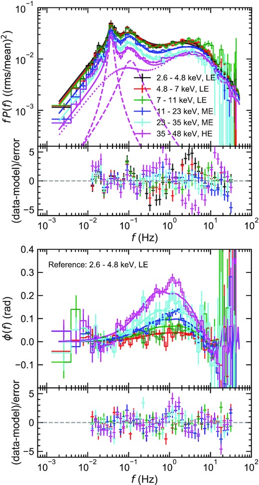
The resulting energy spectrum is shown in Fig. 1 (top). The different colours represent different telescopes (red: LE; green: ME; blue: HE; Zhang et al. 2020). The energy spectrum from ME has a dip of around 22 keV (light green), which is associated with silver fluorescent lines generated within the detector (Li et al. 2020). Following You et al. (2021), we added 1.5 per cent systematic errors to all spectral data.
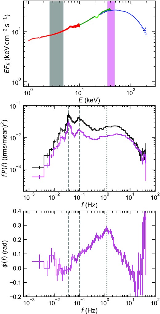
Spectral-timing properties of MAXI J1820+070 observed by Insight-HXMT. Top: time-averaged energy spectrum. Red, green, and blue markers represent LE, ME, and HE telescopes, respectively. The dip around 22 keV (light green) is associated with fluorescent lines of silver generated within the ME detector. The coloured regions show the low (black: 2.6–4.8 keV) and high (magenta: 35–48 keV) used to extract light curves. Middle: power spectra calculated for low- and high-energy bands. Both these have the characteristic double peak shape, but with the QPO and its harmonic (marked with dashed lines) superimposed. The high-energy power spectrum is very similar in shape to that at low energy, but with lower normalization (compare to the model in Fig. 2f). Bottom: phase-lag spectrum between the light curves in the low- and high-energy bands. The lags are defined as positive if variations in higher energy bands lag behind those in lower energy bands (hard lags). The frequency at which the phase lag is maximum is marked with a dotted line. This is substantially lower than the characteristic frequency of the second peak in the power spectrum (compare to the model in Fig. 2h).
To study the fast variability, we split the background-subtracted light curves into segments of |$256\, {\rm s}$| with |$1/128\, {\rm s}$| time bins (215 points), where we avoided any data gaps. We only used the data where all telescopes were active to calculate light curves, using the same time selection for every energy band. We calculate the white-noise-subtracted power spectra and the cross-spectra from each 256 s segment and average them over different segments and logarithmically spaced Fourier frequencies (Uttley et al. 2014; Ingram 2019). All power spectra are normalized such that their integral over frequency corresponds to the fractional variance (Miyamoto et al. 1991; Vaughan et al. 2003). Phase-lag spectra are calculated from the cross-spectra, using the relation between the phase-lag spectrum ϕ(f) and cross-spectrum C(f), ϕ(f) = tan −1(ℑ[C(f)]/ℜ[C(f)]), where ℜ[⋅⋅⋅] and ℑ[⋅⋅⋅] denote the real and imaginary parts, respectively. Phase lag relates to time lag via the relation 2|$\pi$|ft(f) = ϕ(f).
Fig. 1 (middle) shows the power spectra of the 2.6–4.8 keV (black) and 35–48 keV (magenta) light curves These energy bands are marked in the energy spectrum with shaded regions. A quasi-periodic oscillation (QPO) and its harmonic exist around 0.036 and 0.1 Hz (shown with dashed lines), in addition to the broad-band variability.
Fig. 1 (bottom) shows the phase-lag spectrum between these two energy bands. The convention throughout this paper is that positive lags mean that the harder energy band lags behind the softer one. The phase lag peaks at |${\sim}1.2\, {\rm Hz}$| (shown with a dotted line), which is not at the same frequency as the high-energy peak in the power spectra. This is unexpected as simple propagating fluctuations models have the same peak frequency both in the power spectrum and cross-spectrum (Ingram & van der Klis 2013; Rapisarda et al. 2016). The QPO fundamental appears to affect the phase lag between these two energy bands, creating a dip in the phase-lag spectrum around the corresponding frequency (Ma et al. 2021). The effect of the second harmonic on the phase lag is not so clear between these energy bands, but we note it does have an impact on different choices of energy bands (Ma et al. 2021).
For all of the data fits performed in this paper, we use xspec 12.12.1 (Arnaud 1996). We formatted variability data and created a diagonal dummy response such that xspec can import power spectra and phase-lag spectra as a function of Fourier frequency. We developed our model as an xspec model. Being able to perform timing fits with the common tool in spectral fits is beneficial in performing spectral-timing fits. For example, we will perform a joint fit to energy spectrum, six power spectra, and five phase-lag spectra in Section 5. We ignore variability below |${\sim}10^{-2}\, {\rm Hz}$| because it behaves differently from other Fourier frequencies. Yang et al. (2022) interpreted this low-frequency variability as the QPO subharmonic.
3 PROPAGATION AND REVERBERATION IN OUR PREVIOUS MODEL
3.1 Summary of our previous work
We start with a summary of our previous physical model. Fundamentally we assume that variability is generated by fluctuations in density in the flow, which propagate inwards as accretion rate fluctuations. Thus the variability generated at each radius propagates down with the accretion flow so that slower fluctuations generated at large radii imprint on faster fluctuations generated at small radii. These fluctuations in mass accretion rate change the luminosity emitted in the spectrum at that radius.
We then need additional assumptions to turn this into a quantitative model, as we have to assume the form of radial stratification for both the spectrum and variability and how fluctuations are generated and propagated. We expand on each of these below.
We assume a basic geometry that is a truncated disc/hot inner flow, as shown in Fig. 2(a) with emissivity at each radius set by the Shakura–Sunyaev thin disc approximation (Fig. 2b). These two assumptions alone are enough to roughly set the transition radius from the inner edge of the disc to the outer edge of the hot flow by energetics to ∼45Rg, though instead we set this from the QPO frequency, assuming the Lense–Thirring precession (Ingram, Done & Fragile 2009). The similarity of the two estimates gives support to the Lense–Thirring interpretation. In all the following, we use the convention that R = rRg, where Rg = GMBH/c2.
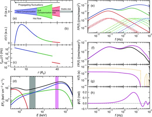
Model set-up and predictions from K22. Here we show only the intrinsic components, rather than including reflection/reverberation, to focus on the physics of the propagation. (a) Assumed accretion flow geometry (height as a function of radius). There is an outer stable disc (grey) that is highly turbulent on its inner edge, forming the variable disc region. Inwards of this is the turbulent hot flow. (b) Radial emissivity, assumed to be similar to that of a thin disc. (c) Frequency at which variability is generated at each radius. There is a discontinuity between the variable disc and hot flow as their scale heights are different, so their characteristic time-scales should be different. Sample parameter values are (Bf, mf) = (4, 1) for the hot flow and (Bd, md) = (0.03, 0.5) for the variable disc. (d) Time-averaged energy spectra modelled (black) assuming a disc for the stable and variable disc emission (red), while the hot flow is assumed to be approximated by two Comptonization components, soft (green) and hard (blue). The relative luminosity in each component, together with the emissivity in (b), roughly sets the size scale of each region, so that the hard Comptonization is for rin–rsh = 6–16, the soft Comptonization for rsh–rds = 16–32, and the variable disc for rds–rout = 32–45. (e) Sample power spectra of the local mass accretion rate in each spectral region. The dashed lines represent the variability generated at each radius, with r = 45, 38, 33 (in the variable disc: red), 30, 22, 16 (in the soft Comptonization: green), and 12, 9, 6 (in the hard Comptonization: blue) from left to right. The frequency, at which each radius fP(f) has its peak, corresponds to the local generator frequency fgen(r). The solid lines show the total (generated plus propagated) variability at r = 38 (red), 22 (green), and 9 (blue). (e) Power spectra for two energy bands highlighted in (d). Any given energy band is not just a single component. The low-energy band (black) contains roughly equal amounts of soft and hard Comptonization, while the high-energy band (magenta) has mostly hard Comptonization, but with some contribution from the soft Comptonization as well. Thus the power spectra of the light curves in the low- and high-energy bands are more similar than those of the soft and hard Comptonization components in (e). None the less, there is still more high-frequency power in the high-energy band than in the low-energy band, but at lower frequencies, the power spectra are identical as both contain the same propagated power. (g) Time-lag spectra for the low- and high-energy band light curves. The orange dotted line shows the intrinsic lag of the soft Comptonization light curve compared to the hard Comptonization light curve. This is ∼50 ms, which is longer than the measured lag of the high-energy band light curve versus the low-energy band due to the mixture of spectral components in each band. (h) Lag between high- and low-energy bands as a phase lag rather than a time lag (related by ϕ(f) = 2|$\pi$|fτ(f)). This peaks around the frequency of the high-energy peak in the power spectrum.
Spectrally, we assume that the flow emits a single component at each radius. This might be unique to each radius, with e.g. each radius in the disc emitting a blackbody with temperature T(R), while the hot flow emits a Comptonized spectrum whose parameters (electron temperature, and optical depth) scale smoothly with radius. However, spectral models are quite degenerate so we approximate the emission from the truncated disc region (rout–rds) as a disc blackbody, and we approximate the hot flow as two zones as physically we do expect that there are two main regions in the flow. Close to the disc, seed photons for Comptonization are predominantly from the disc. However, it is quite easy for this Comptonization to become optically thick along the equatorial direction, shielding the inner regions from the disc photons so that seed photons are predominantly from cyclo-synchrotron (Poutanen & Veledina 2014). Thus we assume that radii from rds–rsh emit soft Comptonization, while radii from rsh–rin emit hard Comptonization (rin < rsh < rds < rout; Fig. 2a and d). Both Comptonization components illuminate the disc to produce reflection, while the energy not reflected is (mostly) thermalized, enhancing the cool disc emission. K22 show that these assumptions give a good fit to the energy spectrum from 0.5 to 80 keV.
As noted above, we assume the QPO is set by the Lense–Thirring precession of the entire hot flow, and the first bump in the power spectrum is set by the turbulent disc (Ingram & Done 2011). This sets (Bd, md) = (0.03, 0.5) and rout = 45.
The dashed lines in Fig. 2(e) show three sample power spectra for the generated variability of the local mass accretion rate in each region (variable disc: red; soft Comptonization: green; hard Comptonization: blue; the middle ring of each highlighted in a darker colour). The functional form is a zero-centred Lorentzian with the cut-off frequency corresponding to the local generator frequency fgen(r), which yields the peak at fgen(r) in the fP(f) representation.
K22 assumed that the propagation time-scale was the same as that on which the fluctuations were generated and called this the viscous time-scale (Lyubarskii 1997; Arévalo & Uttley 2006; Ingram et al. 2009). This assumption sets the propagation speed at any radius vp(r) = rfgen(r) in units of c. However, here we will revisit this assumption, so to avoid confusion, we do not use the term ‘viscous time-scale’ but use ‘generator time-scale’ and ‘propagation time-scale’ in this paper to make it clear which one we mean. K22 also assumed that the fluctuating energy release only changed the normalization of the spectral component emitted at that radius, not its shape.
The solid lines in Fig. 2(e) show the propagated (total) power spectra from each region (disc: red; soft Comptonization: green; and hard Comptonization: blue). This is not the same as the power spectrum in any given energy band as Fig. 2(d) shows that each energy band contains a mix of components.
Fig. 2(f) shows the power spectra for the two chosen energy bands, low (2.6–4.8 keV: black) and high (35–48 keV: magenta), also highlighted in the same colours in Fig. 2(d). While neither band contains the disc emission component, both bands contain the propagated disc variability. The low-energy band also contains both soft and hard Comptonization, so has the generated/propagated power in the soft Comptonization region, plus some of the highest frequency power generated in the hard Comptonization region. The high-energy band is dominated by the hard Comptonization emission, with variability that is propagated down from both the disc and soft Comptonization region, plus the highest frequency power generated/propagated through the hard Comptonization region. Thus the power spectra are almost identical for below |${\sim}1\, {\rm Hz}$|, indicating that variability on these slow time-scales is propagated from the outer regions rather than generated at their emission regions, while they diverge at the highest frequencies where the low-energy band does not include as much of the hard Comptonization component as the high-energy band.
The propagation time-scale is explicitly seen in the time lag (Fig. 2g). The luminosity weighted mean radius of the soft Comptonization band is 22Rg, whereas that for the hard Comptonization band is 11Rg. This lag time (integrating 1/(rfprop(r))) is 51 ms, as seen as the value of the approximately constant time lag at low frequencies (orange dashed line). The time lag drops when the variability starts to be dominated by the generated variability (which is not correlated) rather than the propagated variability, i.e. at approximately the generator time-scale of the hard Comptonization region. At the highest frequencies, the lag also produces oscillatory structure at high frequencies, by the interference generated by the mass accretion rate in the hard Comptonization region being the same as in the soft Comptonization region, but lagged by the mean propagation time-scale. This oscillatory structure has a period of 50 ms. However, the intrinsic lag from the spectral components is diluted by a factor of ∼3 when looking at the low- and high-energy bands rather than the soft and hard Comptonization components. This is because the low-energy band includes both soft and hard Comptonization, while the high-energy band is dominated by the hard Comptonization. While the value of the measured lag time changes, the oscillatory structure period remains at the propagation time-scale.
This oscillation can be seen more clearly in Fig. 2(h), which shows the phase lag rather than time lag, so each time-scale is multiplied by the factor 2|$\pi$|f. In this representation, the phase lag peaks at a frequency between the high-frequency peak in the power spectra at low and high energy. By comparison to the panel above, it is also clear that the oscillatory structure at high frequencies has the same period as in the undiluted (orange) time lags.
All model parameters are summarized in Table 1 and we give a more quantitative model summary in Appendix A.
Summary of our model parameters. The variable flow is spectrally composed of the variable disc region and soft (outer) and hard (inner) Comptonization regions. We call the entire Comptonization region the hot flow.
| Symbol | Meaning | Units | Default |
|---|---|---|---|
| MBH | Black hole mass | M⊙ | 8 |
| Nr | Number of rings splitting the variable flow | 40 | |
| rin | Inner radius of the hard Comptonization | Rg | 6 |
| rsh | Transition radius between the hard Comptonization and soft Comptonization | Rg | 16 |
| rds | Transition radius between the disc and soft Comptonization | Rg | 32 |
| rout | Outer radius of the variable disc | Rg | 45 |
| Fvar,f (Fvar,d) | Fractional intrinsic variability per radial decade in the hot flow (variable disc) | 0.8 | |
| D | Damping factor | 0 | |
| Bf (Bd) | Coefficient of the generator frequency in the hot flow (variable disc) | 0.03 | |
| mf (md) | Power-law index of the generator frequency in the hot flow (variable disc) | 0.5 | |
| |$B^{(\mathrm{p})}_{\mathrm{f}}$| (|$B^{(\mathrm{p})}_{\mathrm{d}}$|) | Coefficient of the propagation frequency in the hot flow (variable disc) | 0.03 | |
| |$m^{(\mathrm{p})}_{\mathrm{f}}$| (|$m^{(\mathrm{p})}_{\mathrm{d}}$|) | Power-law index of the propagation frequency in the hot flow (variable disc) | 0.5 | |
| γ | Power-law index of the emissivity | 3 | |
| b(r) | Inner boundary condition of the emissivity | |$1-\sqrt{r_{\mathrm{in}}/r}$| | |
| t0,h (t0,s) | Time delay of the top hat impulse response of reverberation for the hard (soft) Comptonizationa | s | 5.5 × 10⁻³ |
| Δt0,h (Δt0,s) | Time duration of the top hat impulse response of reverberation for the hard (soft) Comptonizationa | s | 10 × 10−3 |
| S0(E) | Fractional contribution of spectral components to the fluxb,c,d | 0.5 | |
| η0,h (η0,s) | Constant term of the sensitivity of the hard (soft) Comptonization to change in mass accretion ratee | 1 | |
| η1,h (η1,s) | Gradient term of the sensitivity of the hard (soft) Comptonization to change in mass accretion ratee | 0 |
aParameters are required when the reverberation is considered.
bEach spectral component has its own parameter: S0(E) consists of Sd(E), Ss(E), |$S^{(\mathrm{r})}_{\mathrm{s}}(E)$|, Sh(E), and |$S^{(\mathrm{r})}_{\mathrm{h}}(E)$| (see Section 3).
cS0(E) is replaced by η(E)S0(E) for timing fits when the spectral pivoting is included (Section 4.2).
dS0(E) is calculated from spectral models for spectral-timing fits (Section 5).
eParameters are required for spectral-timing fits (Section 5).
The fluctuating soft and hard Comptonization regions illuminate the outer disc and produce a reflected/reprocessed signal that lags behind the generated and propagated flow variability by the light travel time to the disc. The reflected emission itself is not strong, though this real reverberation signal will add to the soft lags produced by interference in the propagation (hard) lags seen in Fig. 2(g). However, at lower energies, the photons that are not reflected heat the disc, giving a thermal reverberation signal that is strong at energies close to that of the disc emission (|${\lesssim}2\, {\rm keV}$|; Kara et al. 2019). This reverberation signal gives an independent check on the assumption of the disc truncation radius, and the fact that it is consistent (De Marco et al. 2021) gives strong supporting evidence for the underlying assumption that the QPO mechanism is the Lense–Thirring precession. Our previous model includes the reverberation, along with the propagating fluctuations (K22).
K22 showed that this model gave a fairly good fit to the energy dependence of the power spectrum across the NICER energy band (0.5–10 keV) and to the lags between the same fluctuations in different energy bands as a function of frequency. However, while the spectral components were built from NuSTAR data, which extended above 10 keV, this instrument does not have a sufficient area to do high-time-resolution studies, so the model prediction at higher energies could not be tested.
This outburst of MAXI J1820+070 was also monitored by Insight-HXMT (Ma et al. 2021; You et al. 2021; Yang et al. 2022), which does have a sufficient effective area at high energies. As mentioned in the previous section, the Insight-HXMT data are not absolutely simultaneous with the NICER/NuSTAR data set we used in K22, but they are very close in time, and spectral-timing properties are nearly constant during these periods. Hence we take the spectral-timing model of K22, use it to predict the higher energy behaviour, and compare it to the Insight-HXMT data.
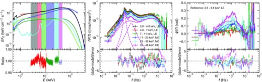
3.2 Comparison of our previous model to Insight-HXMT data
We compare the predictions of our previous model to the power spectra for the 2.6–4.8 and 35–48 keV bands and the phase-lag spectrum between these bands calculated from the Insight-HXMT observation data in Fig. 3 (left). Model parameter values are summarized in Table 2, which also contains those for the rest of the columns in Fig. 3. The lower energy band is well reproduced by our previous model from K22, as expected, as it is within the NICER energy range over which K22 got good fits. However, the power spectrum at the higher energy band is clearly overestimated, and the phase lag between the two is completely wrong, peaking at too high a frequency with a lag that is too short to match the data.
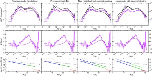
The effect of the model updates on the timing properties. Each figure shows the low (2.4–4.8 keV: black) and high (35–48 keV: magenta) energy band power spectra (upper) and phase-lag spectra (middle), with data shown as the stepped line with errors and the model as the smooth curve. The lower panel shows the propagation frequency (solid) and generator frequency (dashed) used in the model calculations, with the Keplerian frequency (dash–dotted) for reference. Left: predictions from the previous model from K22 (Section 3) built from a full spectral-timing fit to the 0.5–10 keV data. Mid-left: fitting with the previous model (Section 3), ignoring the time-averaged spectrum. Mid-right: extending the model to include a different propagation and generator time-scale (Rapisarda et al. 2017). This shifts the frequency of the phase-lag peak but does not change the power spectra. We also gave the model the freedom to include damping (Mahmoud & Done 2018b), but the best-fitting value was close to zero, so this is not shown (Section 4.1). Right: including spectral pivoting and a difference in generator and propagation time-scale (Section 4.2). This allows the power spectral normalization of the high-energy band to be lower than at low energies, giving a significant improvement in the consistency of the model calculations.
Model parameter values used in Fig. 3. Common parameter values used in all fitting are MBH = 8, Nr = 40, rin = 6, rout = 45, |$B_{\mathrm{d}}=B^{(\mathrm{p})}_{\mathrm{d}}=0.03$|, |$m_{\mathrm{d}}=m^{(\mathrm{p})}_{\mathrm{d}}=0.5$|, γ = 3, and |$b(r)=1-\sqrt{r_{\mathrm{in}}/r}$|. The transition radii are fixed to rsh = 17.8, rds = 32.1 for the left-hand column and rsh = 16, rds = 32 for other columns, although these differences are too subtle to become important. Other constraints are Fvar,f = Fvar,d and D = 0. The mark ‘(f)’ means that a value of the corresponding parameter is fixed.
| Symbol | Left | Mid-left | Mid-right | Righta |
|---|---|---|---|---|
| Fvar,d | 0.8 (f) | 0.53 | 0.59 | 0.8 (f) |
| Bf | 6 (f) | 11.9 | 342 | 560 |
| mf | 1.2 (f) | 1.50 | 2.42 | 2.73 |
| |$B^{(\mathrm{p})}_{\mathrm{f}}$| | =Bf | =Bf | 80.1 | 166 |
| |$S_\mathrm{d}(2.6\textrm {--}4.8\, {\rm keV})$| | 0.001 (f) | 0 (f) | 0 (f) | 0 (f) |
| |$S_\mathrm{s}(2.6\textrm {--}4.8\, {\rm keV})$| | 0.356 (f) | 0.505 | 0.471 | 0.305 |
| |$S_\mathrm{h}(2.6\textrm {--}4.8\, {\rm keV})$| | 0.330 (f) | =1 − Ss(E) | =1 − Ss(E) | 0.571 |
| |$S^{(\mathrm{r})}_\mathrm{s}(2.6\textrm {--}4.8\, {\rm keV})$| | 0.307 (f) | 0 (f) | 0 (f) | 0 (f) |
| |$S^{(\mathrm{r})}_\mathrm{h}(2.6\textrm {--}4.8\, {\rm keV})$| | 0.006 (f) | 0 (f) | 0 (f) | 0 (f) |
| |$S_\mathrm{d}(35\textrm {--}48\, {\rm keV})$| | 0 (f) | 0 (f) | 0 (f) | 0 (f) |
| |$S_\mathrm{s}(35\textrm {--}48\, {\rm keV})$| | 0.213 (f) | 0.348 | 0.277 | −0.056 |
| |$S_\mathrm{h}(35\textrm {--}48\, {\rm keV})$| | 0.474 (f) | =1 − Ss(E) | =1 − Ss(E) | 0.476 |
| |$S^{(\mathrm{r})}_\mathrm{s}(35\textrm {--}48\, {\rm keV})$| | 0.134 (f) | 0 (f) | 0 (f) | 0 (f) |
| |$S^{(\mathrm{r})}_\mathrm{h}(35\textrm {--}48\, {\rm keV})$| | 0.179 (f) | 0 (f) | 0 (f) | 0 (f) |
a|$S_{0}(E)$| means η(E)S0(E) in this column.
4 TIMING FITS: EXPLORING THE ADDITIONAL PROCESSES REQUIRED TO MATCH THE HIGH-ENERGY VARIABILITY
Finally, we only have the soft and hard Comptonization components with the constraints of Ss(E) + Sh(E) = 1. We do not include any models for the QPO features for simplicity.
We keep the black hole mass of MBH = 8 M⊙ (Torres et al. 2020) and emissivity profile, i.e. γ = 3 and |$b(r)=1-\sqrt{r_{\mathrm{in}}/r}$| (Novikov & Thorne 1973; Shakura & Sunyaev 1973), where we assume that radiation energy from the annulus ranging from r to r + Δr is proportional to r−γb(r)2|$\pi$|rΔr. In K22, the transition radii rsh, rds were calculated from the emissivity profile and spectral decomposition. However, we lack spectral decomposition. In addition, it turned out that model calculations are hardly affected by small changes in these parameters. Thus, we simply fix these transition radii to typical values, rsh = 16 and 32.
We show the result of the joint fit to the power spectra for 2.6–4.8 and 35–48 keV and the phase-lag spectrum between these energy bands in Fig. 3 (mid-left). The fit is not qualitatively improved even giving the K22 model maximal freedom to fit without constraints from the time-averaged energy spectrum. The K22 model always has a high-energy-band power spectrum similar to that in the low-energy band everywhere except at the highest frequencies. Yet the data have very different power spectral normalizations even at low frequencies where propagation should dominate.
Plainly, while the previous model from K22 was designed to fit the data below 10 keV, it does not extrapolate to the higher energies, so does not adequately describe the physics of the propagation of fluctuations through the flow. This is important as K22 show that the propagation speed is a key determinant of the nature of the hot flow, which can allow large-scale magnetically dominated flows (magnetically arrested disc – MAD) to be distinguished from those with turbulent dynamo (standard and normal evolution – SANE) models. The poor applicability of our previous model to higher energy bands motivates our study to improve it.
4.1 Suppressing variability at high energies with a constant spectral shape
The major feature missing in the previous model for the power spectra is the strong suppression of fractional variability at high energies. The generation/propagation of fluctuations in the model, where slower fluctuations generated outer regions propagate down through the flow, always leads to an increase in variability with energy, as long as the spectrum hardens inwards. In contrast, the Insight-HXMT observation data show that plainly the high-energy broad-band power spectrum is a factor of ∼3 lower than the low-energy power spectrum at all frequencies (Fig. 1, middle). This decrease in fractional variability with energy was not seen in the NICER energy band (|${\lesssim}10\, {\rm keV}$|; K22). But it has been seen before, in e.g. the RXTE data of other black hole binary low/hard states (e.g. Nowak et al. 1999; Axelsson & Done 2018 for Cyg X-1; Malzac et al. 2003 for XTE J1118+480). In the context of other propagating fluctuations models, it was modelled by the damping of high-frequency fluctuations as they propagate inwards (Arévalo & Uttley 2006; Rapisarda et al. 2017), and by decreasing the intrinsic variability power generated in the inner regions (Mahmoud & Done 2018b). To implement these effects in our model, we introduce two new parameters. One is a damping parameter D, which suppresses high-frequency variability by exp(−DfΔt), where Δt is the propagation time. The damping effect is ignored if D = 0. We also allow the intrinsic variability amplitude to be different between the hot flow Fvar,h and disc Fvar,d (the previous model from K22 has Fvar,f = Fvar,d).
The modified model formalism due to the damping effect is given in Appendix B. Other additional effects, Fvar,d ≠ Fvar,f and fgen(r) ≠ fprop(r), just alter the power spectrum of intrinsic mass accretion rate variability at nth ring |A(rn, f)|2 (equation A1) and the propagation time from the outer kth ring to the inner nth ring Δtk, n (equation A3), respectively, without affecting any other equations containing |A(rn, f)|2 and Δtk, n. As in the last part of the previous section, we attempt to reproduce only variability properties based on the propagating fluctuations process rather than full spectral timing. We keep those parameters fixed that are fixed in the previous fit.
Even with all these additional effects, the model is still not capable of matching the observation data. The damping parameter D is pegged to its lower bound of zero, indicating that the damping described above is ineffective in improving the fit (Mahmoud et al. 2019). This is because our model assumes that the intrinsic variability has a cut-off at the local generator frequency fgen(r), as shown in Fig. 2(c). This assumption already includes some aspects of damping. The MRI (Balbus & Hawley 1991, 1998) is expected to produce variability up to quite fast time-scales. However, only variability slower than the local propagation time can propagate inwards as the faster variability is viscously damped out (Churazov, Gilfanov & Revnivtsev 2001; Cowperthwaite & Reynolds 2014; Hogg & Reynolds 2016; Ingram 2016; Bollimpalli et al. 2020; Turner & Reynolds 2021). Our assumptions about the intrinsic variability are an approximation of this physical picture. The damping parameter being pegged to zero indicates there is no need for additional damping effects. We did not find an improvement in the fits using separate variability amplitude between the variable disc region and hot flow region, either.
Fig. 3 (mid-right) shows the results of a joint fit to the power spectra for 2.6–4.8 and 35–48 keV and the phase-lag spectrum between these energy bands by allowing fgen(r) ≠ fprop(r) for the hot flow. For clarity, we removed the other additional effects that did not make a difference, i.e. Fvar,d = Fvar,f and D = 0.
Although we see a slightly better match to the observed peak frequency of the phase-lag spectrum than the previous fit, the model still underestimates its amplitude. More importantly, we still do not solve the essential issue: the model calculates similar or larger variability for higher energy bands, inconsistent with the observation that the power spectral amplitude is larger for the lower energy band. Mahmoud & Done (2018b) and Mahmoud et al. (2019) introduce more complex radial dependence for the intrinsic variability, emissivity, and damping to capture energy-dependent variability properties. However, some assumptions involved with these complications remain to be tested. We do not explore the complex radial structure further and conclude that those additional effects implemented here are less effective than required by the high signal-to-noise ratio data obtained by Insight-HXMT.
We note that the difficulty in reproducing the observation data here lies in joint fitting to the power spectra and phase-lag spectrum. It is possible to reproduce power spectra for these energy bands with the current model fairly well, ignoring the phase-lag spectrum. In this case, however, the lower energy photons would come from inner regions, because inner regions are more variable than outer regions, and predict soft lags, which is completely in disagreement with the observed hard lags. This points to the importance of modelling cross-spectra and power spectra.
4.2 Spectral pivoting
So far, we have assumed that the spectral shape of each component does not vary in time. However, this is unphysical because mass accretion rate fluctuations make spectral parameters, e.g. the optical depth and electron temperature, vary on short time-scales (Malzac et al. 2003; Gandhi et al. 2008; Yamada et al. 2013; Bhargava et al. 2022). This oversimplification limits the model’s flexibility to reproduce energy-dependent variability data. Hence we now allow the spectral shapes to fluctuate (Veledina 2016, 2018; Mastroserio et al. 2018, 2019, 2021), along with their amplitude. The schematic picture of the spectral pivoting is shown in Fig. 4 (top).
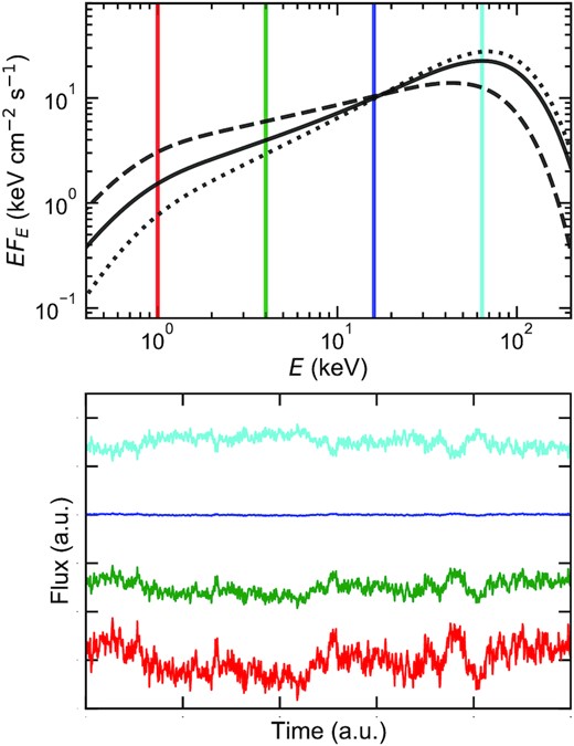
Schematic picture of the effect of spectral pivoting as implemented here. Top: instant local energy spectra when the mass accretion rate at the corresponding radius is higher than, equal to, and lower than the average (dashed, solid, and dotted, respectively). Bottom: light curves of the local flux for different energies, |$1\, {\rm keV}$| (red), |$4\, {\rm keV}$| (green), |$16\, {\rm keV}$| (blue), |$64\, {\rm keV}$| (cyan) as marked in the top panel. Each light curve is normalized by its average and offset for clarity. The light curves in the lower energy bands (red and green) are positively correlated with the local mass accretion rate, but the fluctuations have lower amplitude as the energy increases, going to zero at the pivot point at 16 keV, and then switching to negative correlation at higher energies (cyan).
Here, we give concise explanations of how the spectral pivoting is implemented and what the model gets to be able to handle with this update. More detailed formalism is found in Appendix C. A constant spectral shape means that the spectrum at every energy reacts to mass accretion fluctuations in the same way. We consider the mass accretion rate and energy spectrum at a certain radius. By defining the average and difference from the average as |$\dot{m}_0$| and |$\Delta \dot{m}(t)$| for the mass accretion rate and as S0(E) and ΔS(E, t) for the spectrum, the constant spectral shape is equivalent to |$\Delta S (E, t)/S_0 (E)=\Delta \dot{m} (t)/\dot{m}_0$|, which is independent of energy E. To let the spectral shape vary in time, we give the spectrum sensitivity to |$\Delta \dot{m}(t)$| as a function of energy, η(E), and redefine |$\Delta S (E, t)/S_0 (E)=\eta (E) \Delta \dot{m} (t)/\dot{m}_0$|, which now depends on energy. The amplitude of sensitivity parameter |η(E)| regulates how sensitive the spectrum is to a change in the mass accretion rate from its average, while its sign determines whether the spectrum reacts positively or negatively. The spectrum gets higher (lower) with an increase in mass accretion rate if η(E) > 0 (<0). The energy at which η(E) crosses zero, called the pivoting point, does not react to a change in mass accretion rate. Light curves of local flux for different energies are illustrated in Fig. 4 (bottom). We note that we do not simulate light curves in the model calculations. The decrease in η(E) with energy, i.e. the spectrum being less sensitive to |$\Delta \dot{m}(t)$| for higher energies, could let the power spectrum decrease with energy, as observed for MAXI J1820+070, even if the mass accretion rate is more variable for central regions emitting higher energy photons. In our implementation, there arises no lag between different energies from the spectral pivoting itself except for the phase lag of |$\pi$| when η(E1)η(E2) < 0. Our new model shares this feature of spectral pivoting with the model developed by Veledina (2016, 2018). The new model returns to the previous one by setting η(E) = 1.
Each spectral component is expected to show its own sensitivity pattern. We give the sensitivity parameter to each spectral component, |$\eta _{\mathrm{Y}}(E)\, (\mathrm{Y}={\mathrm{d, s, h}})$|, where the subscripts stand the variable disc, soft Comptonization, and hard Comptonization, respectively. With the implementation of spectral pivoting, all |$S_{\mathrm{Y}}(E)\, (\mathrm{Y}={\mathrm{d, s, h}})$| contained in the analytic expressions of power spectra and cross-spectra is replaced by ηY(E)SY(E) (see Appendix C for the derivation). This means that the model’s flexibility is not bound by the constraint (3) anymore because time-averaged spectra always appear as the product with their sensitivity. In addition, ηY(E)SY(E) can be negative in contrast to 0 ≤ SY(E) ≤ 1. The spectral pivoting gives freedom to the model in this way.
We attempt to fit the variability properties with the new model. We have ηY(E)SY(E) as model parameters, instead of SY(E). The negligible disc emission Sd(E) = 0 results in ηd(E)Sd(E) = 0. We fix D = 0, in which all intrinsic variability propagates inwards without any loss. We also fix Fvar,d = Fvar,f to the typical value of 0.8 because the sensitivity parameter η(E) can regulate the variability amplitude.
The simultaneous fit to the power spectra for 2.6–4.8 and 35–48 keV and the phase-lag spectrum between these energy bands with the new model is shown in Fig. 3 (right). We see significant improvement in variability modelling by allowing the spectral shapes to vary in time. Our new model captures the energy-dependent variability, pointing to the importance of spectral pivoting in modelling variability at high energies.
Joint fit to six power spectra (top) and five phase-lag spectra (bottom) across 2.6–48 keV with our new model including the spectral pivoting. We include two Lorentzian functions for the QPO (dashed) and harmonic (dotted). In the calculation of phase-lag spectra, the lowest band of 2.6–4.8 keV is chosen as the reference band. The lower plot for each panel is the difference between data and model divided by 1σ errors. The new model including the spectral pivot successfully reproduces all the timing data across this bandpass.
| Symbol | Value |
|---|---|
| Fvar,d | 0.8 (f) |
| Bf | 401 |
| mf | 2.59 |
| |$B^{(\mathrm{p})}_{\mathrm{f}}$| | 108 |
| |$\eta _{\mathrm{s}} S_\mathrm{s}(2.6\textrm {--}4.8\, {\rm keV})$| | 0.315 |
| |$\eta _{\mathrm{h}} S_\mathrm{h}(2.6\textrm {--}4.8\, {\rm keV})$| | 0.588 |
| |$\eta _{\mathrm{s}} S_\mathrm{s}(4.8\textrm {--}7\, {\rm keV})$| | 0.242 |
| |$\eta _{\mathrm{h}} S_\mathrm{h}(4.8\textrm {--}7\, {\rm keV})$| | 0.601 |
| |$\eta _{\mathrm{s}} S_\mathrm{s}(7\textrm {--}11\, {\rm keV})$| | 0.189 |
| |$\eta _{\mathrm{h}} S_\mathrm{h}(7\textrm {--}11\, {\rm keV})$| | 0.617 |
| |$\eta _{\mathrm{s}} S_\mathrm{s}(11\textrm {--}23\, {\rm keV})$| | 0.116 |
| |$\eta _{\mathrm{h}} S_\mathrm{h}(11\textrm {--}23\, {\rm keV})$| | 0.549 |
| |$\eta _{\mathrm{s}} S_\mathrm{s}(23\textrm {--}35\, {\rm keV})$| | 0.049 |
| |$\eta _{\mathrm{h}} S_\mathrm{h}(23\textrm {--}35\, {\rm keV})$| | 0.498 |
| |$\eta _{\mathrm{s}} S_\mathrm{s}(35\textrm {--}48\, {\rm keV})$| | −0.052 |
| |$\eta _{\mathrm{h}} S_\mathrm{h}(35\textrm {--}48\, {\rm keV})$| | 0.484 |
| χ2/degrees of freedom | 1095.0/457 |
We find that the new model matches observations well for all energy bands whilst keeping parameter values similar to those found in the joint fitting for 2.4–4.8 and 35–48 keV only (Fig. 3, right). It is interesting to note that the spectral parameter for the soft Comptonization component μs(E)Ss(E) decreases with energy and finally reaches a negative value at the highest energy band of 35–48 keV. This means that the soft Comptonization component increases for an increase in mass accretion rate at low energies (|${\lesssim}35\, {\rm keV}$|), whereas it decreases at high energies (|${\gtrsim}35\, {\rm keV}$|), showing the pivoting point of |${\sim}35\, {\rm keV}$|.
Although the broad-band variability has been studied with Insight-HXMT observations (e.g. Wang et al. 2020; Yang et al. 2022), we succeeded in reproducing it with a physically motivated model for the first time. In addition, while propagating fluctuations models have been applied up to |${\sim}35\, {\rm keV}$| (Mahmoud & Done 2018a,b) with RXTE observations, we extend the energy range up to 48 keV using Insight-HXMT observations with significantly improved residuals. Our successful modelling shows the propagating fluctuations scenario holds good up to high-energy bands, keeping it the most plausible explanation for the aperiodic variability.
5 JOINT SPECTRAL-TIMING FIT WITH SPECTRAL PIVOTING
To connect the time-averaged spectrum and variability consistently, we take reverberation into account in our timing model. Its implementation is updated from that in K22 mainly due to the inclusion of spectral pivoting. We summarize how the reverberation behaves in our new model here, while the detailed formalism is described in Appendix D.
The illuminating Comptonization spectrum changing its shape with time results in the reflected spectrum also changing its shape with time. As in the previous section, we consider a certain radius. Along with the mass accretion rate and direct emission, we account for the reflected emission associated with the direct emission. Defining the average and difference from it as |$S^{(\mathrm{r})}_{0}(E)$| and ΔS(r)(E, t), we assume |$\Delta S^{(\mathrm{r})}(E, t)/S^{(\mathrm{r})}_{0}(E) = (\Delta S(E, t)/S_{0}(E))\otimes h(t)=\eta (E) (\Delta \dot{m}_{0}(t)/\dot{m}_{0})\otimes h(t)$|. We use the superscript ‘(r)’ to stand for the reflected emission. The convolution in time is denoted by ⊗, and h(t) is called the impulse response, which is the time evolution of reflected emission for a flash of illumination. All information as to the disc response, such as the delay for the direct emission due to an additional light crossing path and the duration due to the different delay times for different locations of reflection, are encoded in h(t).
The relation of spectral variation between the direct and reflected emission means that the reflected emission follows variations of the direct emission at the corresponding energy with some time delay, as long as the variability is slow enough not to be washed out via reprocessing, i.e. via the operation of the convolution. In the simple case of h(t) = δ(t − τ), variations of the reflected emission exactly lag behind those of the direct emission with the time delay of τ: |$\Delta S^{(\mathrm{r})}(E, t)/S^{(\mathrm{r})}_{0}(E)=\Delta S(E, t-\tau)/S_{0}(E)$|.
We note the difference in the model calculations between the timing fits (Section 4.2) and spectral-timing fits. In the timing fits, η(E)S0(E) is a model parameter, and it is impossible to disentangle this product. On the other hand, S0(E) and η(E) are separately modelled in the spectral-timing fits. The former is calculated from spectral models, the latter is from equation (9).
In the joint spectral-timing fit, we fix the seed photon temperature of Comptonization components to the typical disc temperature in this state, |$kT_{\mathrm{seed, s}}=kT_{\mathrm{seed, h}}=0.2\, {\rm keV}$| (De Marco et al. 2021; K22). Since the electron temperature is difficult to constrain from the energy band of interest, we fix it to |$kT_{\mathrm{e, s}}=kT_{\mathrm{e, h}}=23\, {\rm keV}$|, as in K22. While we allow the inner radius of the reflector for the hard Comptonization component to be free, we fix that for the soft Comptonization component to Rin,s = 45Rg corresponding to the outer edge of the variable flow located at rout = 45. Following K22, we fix the inclination angle to i = 66° (Torres et al. 2020) and Fe abundance to ZFe = 1.1. We also set the black hole spin to a* = 0, consistent with rin = 6 in the timing model, and use the high electron density of |$N_{\mathrm{e}}=10^{20}\, {{\rm cm}^{-3}}$| (García et al. 2016; Mastroserio et al. 2021). The delay and duration of the impulse response are, in principle, derived from the location and geometry of illuminating source and reflector. However, in the geometry assumed, the time-scales of reverberation |${\lesssim}10\, {\rm ms}$| (corresponding to the light crossing of ≲250Rg for MBH = 8 M⊙) are shorter than variability time-scales of interest (|$20\, {\rm ms}\textrm {--}100\, {\rm s}$|). In addition, reverberation signatures are unclear across the energy bands of interest (|$2.6\textrm {--}48\, {\rm keV}$|), and small alterations of the impulse response due to small changes of the accretion flow geometry do not significantly affect the variability properties. Thus, we simply fix |$t_{0, \mathrm{s}}=t_{0, \mathrm{h}}=6\, {\rm ms}$| and |$\Delta t_{0, \mathrm{s}}=\Delta t_{0, \mathrm{h}}=10\, {\rm ms}$| as typical values. The top-hat impulse response with these values appears to be good approximations of more realistic ones (K22).
The results of simultaneous modelling of the energy spectrum, six power spectra, and five phase-lag spectra are shown in Fig. 6. The comparison between the data and model is also plotted as the ratio for the energy spectrum and the difference divided by 1σ errors for the variability. Model parameter values are found in Table 4. Overall, our new model successfully reproduces both time-averaged and variability properties, although the discrepancies are seen in the phase-lag spectrum between 35–48 and 2.6–4.8 keV (magenta), which is discussed in Section 6.3. This modelling is the first simultaneous fit to spectrum and variability using our model. The uncertainties of the derived parameter values are evaluated with a Markov chain Monte Carlo (MCMC) analysis in Appendix E.
Spectral-timing fit to the time-averaged energy spectrum (left), six power spectra (middle), and five phase-lag spectra (right) across 2.6–48 keV with our new model including spectral pivoting. In the left-hand panel, the soft Comptonization and its associated reflection are plotted with the green and light green lines, while the hard Comptonization and its associated reflection are plotted with the blue and light blue lines. The black line shows their sum. We include the effect of galactic absorption of |$N_{\mathrm{H}}=1.4 \times 10^{21}\, {{\rm cm}^{-2}}$| on the spectral components. The colours of the shaded regions in the energy spectral plot show the energy band used in the power spectra and phase-lag spectra. In the middle panel, the power spectrum at the highest energy band includes the QPO and harmonic, as in Fig. 5. The bottom panels show residuals. The data-to-model ratio is used for the energy spectrum, while the difference between data and model divided by 1σ errors is used for power spectra and phase-lag spectra. We successfully fit all the data in this bandpass with our updated model including the spectral pivoting, except for a slight underestimate of the phase-lag spectrum around the peak for the highest energy band.
Model parameter values derived from the joint spectral-timing fit in Fig. 6. Fixed parameters related to the spectrum are the seed photon temperature |$kT_{\mathrm{seed, s}}=kT_{\mathrm{seed, h}}=0.2\, {\rm keV}$|, electron temperature |$kT_{\mathrm{e, s}}=kT_{\mathrm{e, h}}=23\, {\rm keV}$|, Fe abundance ZFe = 1.1, inclination angle i = 66°, black hole spin a* = 0, electron density |$N_{\mathrm{e}}=10 ^{20}\, {{\rm cm}^{-3}}$|, inner radius of reflection region Rin,s = 45Rg, and outer radii of reflection region Rout,s = Rout,h = 1000Rg. The subsubscript ‘s’ (‘h’) denotes the soft (hard) Comptonization or its associated reflection component. Fixed parameters related to variability are the same as in Table 2 in addition to the extra parameters about reverberation, |$t_{0, \mathrm{s}}=t_{0, \mathrm{h}}=6\, {\rm ms}$| and |$\Delta t_{0, \mathrm{s}}=\Delta t_{0, \mathrm{h}}=10\, {\rm ms}$|.
| Component | Model | Symbol | Value |
|---|---|---|---|
| Spectral parameters | |||
| Soft Comptonization and reflection | nthcomp | Γs | 1.81 |
| norms | 1.38 | ||
| relxillCp | log10ξs | 3.44 | |
| |$\mathrm{norm}^{(\mathrm{r})}_{\mathrm{s}}$| | 0.0395 | ||
| Hard Comptonization and reflection | nthcomp | Γh | 1.50 |
| normh | 2.11 | ||
| relxillCp | Rin,h | 78 | |
| log10ξh | 1.70 | ||
| |$\mathrm{norm}^{(\mathrm{r})}_{\mathrm{h}}$| | 0.0328 | ||
| Variability parameters | |||
| Broad-band | Our model | Bf | 862 |
| mf | 2.81 | ||
| |$B^{(\mathrm{p})}_{\mathrm{f}}$| | 189 | ||
| η0,s | 1.023 | ||
| η1,s | −0.568 | ||
| η0,h | 1.527 | ||
| η1,h | −0.580 | ||
| χ2/d.o.f. | 1993.1/1795 | ||
The spectral variation derived from the fit is shown in Fig. 7. The spectra for the mass accretion rate being its average and double the average are plotted with solid and dashed lines. For illustration purposes, we ignore all effects from the impulse response for reverberation, such as time delay, i.e. we assume h(t) = δ(t). This means that the Comptonization and its associated reflection behave completely in the same way, |$\Delta S(E, t)/S_{0}(E)=\Delta S^{(\mathrm{r})}(E, t)/S^{(\mathrm{r})}_{0}(E)$|. Generally, all spectra are less sensitive for higher energies to mass accretion rate fluctuations, which results in a decrease in the power spectrum with energy. We see the pivoting point at |${\sim}50\, {\rm keV}$| for the soft Comptonization and its reflection, which roughly agrees with that at |${\sim}35\, {\rm keV}$| derived from the fit only to the timing properties in the previous section.
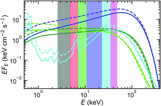
Changes in the shape of the energy spectral components due to changes in mass accretion rate derived from the spectral-timing fit in Fig. 6. The average energy spectrum for the soft (green) and hard (blue) Comptonization components and their reflected emission (pale green and cyan, respectively) are shown as solid lines, while the dashed lines show the effect of doubling the mass accretion rate.
6 DISCUSSION
6.1 Generator time-scale and propagation time-scale
The characteristic time-scales on which the fluctuations are propagated at each radius are derived from the spectral-timing fit (Fig. 6). We compare the propagation frequency derived (solid) to those predicted by different hot flow models (dash–dotted) in Fig. 8. The theoretical propagation frequencies for the advection-dominated accretion flow (ADAF; Narayan, Kato & Honma 1997), standard and normal evolution (SANE; Narayan et al. 2012), magnetically arrested disc (MAD; Narayan et al. 2012), and jet emitting disc (JED; Marcel et al. 2018) are calculated in a standard way by dividing the accretion speed by radius assuming MBH = 8 M⊙ (see K22 for details). The propagation frequency derived from our previous model from K22 is also plotted (dashed).
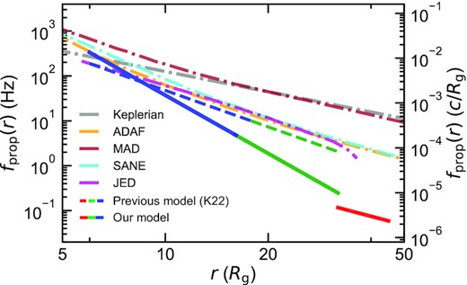
Propagation frequency (solid) as a function of radius derived from the spectral-timing fit. Red, green, and blue colours denote the variable disc, soft Comptonization, and hard Comptonization regions, respectively. The propagation frequency derived from our previous work and predicted from theoretical models are plotted with a dashed line and dash–dotted lines (see K22 for details). A black hole mass of MBH = 8 M⊙ is assumed. The Keplerian frequency is also plotted with a grey dash–dotted line for reference. We caution that none of these models except the JED-SAD has an explicit transition from the flow to the disc.
In K22, we found fairly good agreement of the derived propagation time-scales with those in ADAF, SANE, and JED rather than MAD. The propagation time-scale derived from our new model is now not very similar to any theoretical predictions. Here, allowing the generator and propagation frequencies to be different makes their radial dependence steeper, i.e. from fprop(r) ∝ r−2.7 to fprop(r) ∝ r−4.31. This steep radial dependence is required to reproduce both the observed large phase lags and high-frequency broad-band variability simultaneously. Indeed, the propagation time-scale derived is robust against uncertainties of the relationship between the generator time-scale and propagation time-scale. Using our new model including the spectral pivoting, the assumption of fgen(r) = fprop(r) also gives a similar propagation time-scale, although the fit is not as good as that obtained in the previous section with fgen(r) ≠ fprop(r). The key feature that our new model requires is a slow propagation speed enough to reproduce observed phase lags. The propagation time-scale of MAD (brown dash–dotted line) is too short to explain the observed phase lags. Thus, our results still prefer SANE rather than MAD, although MAXI J1820+070 displays a powerful jet (Bright et al. 2020).
6.2 Origin of QPOs
Our full spectral-timing modelling accounts for all the X-ray spectrum and rapid variability except for the QPOs. We model these QPOs by adding peaked Lorentzian components in the power spectra. No extra component is added to the phase-lag spectra simply because the QPO features are not very clear across 2.6–48 keV. We did not add any other spectral components for the QPOs, implicitly assuming that the QPO is a modulation of the spectral components already included in the model (multiplicative) rather than being associated with an additional spectral component (additive).
Our successful modelling does not give much room for an additional emission component only related to the QPOs (Fig. 6), supporting the assumption above. This result is consistent with a QPO produced predominantly from a global mode of flow rather than an intrinsic change in intensity with QPO frequency. We specifically have in mind the Lense–Thirring (vertical) precession of the entire hot flow, where the observed luminosity of the Comptonization component(s), including all their stochastic variability, are modulated by the changing projected area of the translucent hot flow as the viewing angle changes with QPO phase (Fragile et al. 2007; Ingram et al. 2009; Ingram & Done 2011, 2012). This picture agrees with the new polarization results for Cyg X-1 in the low/hard state, which requires the hot X-ray emitting plasma to be radially extended (Krawczynski et al. 2022). Conversely, the alternative model of a precessing jet suggested by Ma et al. (2021) is challenged by the polarization results because it requires the hot X-ray emitting region to align with the jet.
6.3 Limitations of our new model
Our new model gives a poor fit to both the energy spectrum and phase lags beyond ∼40–50 keV. From Fig. 6 (left), the spectral model clearly underestimates the data above ∼100 keV. The hard Comptonization spectrum rolls over too fast to match the observed data. The comparison of the phase-lag spectrum between the model and data at high energies is shown in Fig. 9. The model phase lags increase smoothly with energy to |${\sim}40\, {\rm keV}$| (Fig. 6, right) but then saturates to a constant value rather than continually increasing as in the data. The lag behaviour arises as the fraction of the total spectrum that is made of the hard (and long lagged) Comptonization spectrum increases up to around |${\sim}40\, {\rm keV}$|, but after this point, the hard Comptonization dominates, leading to the saturation of lag.
The predicted high-energy phase lags (lines) versus the data (points), calculated using the standard 2.6–5.8 keV reference band. The lowest energy band on this plot is 35–48 keV (magenta), which is the highest energy band included in the spectral-timing fits. The predicted phase lags at higher energies saturate beyond 40 keV, unlike the data, which show a clear increase in phase lag with energy, pointing out the limitations of the model.
The spectral mismatch could be fixed if there is additional stratification of the energy spectrum of the hot flow, so the very innermost regions produce an even hotter/harder Comptonization component. In many ways, this is quite natural. The two Comptonization components used here for the spectral decomposition are only an approximation to a continuous flow with (presumably) continuous stratification, even if we do expect there physically to be two main regions. Close to the disc, seed photons for Comptonization are predominantly from the disc. However, it is quite easy for this Comptonization to become optically thick along the equatorial direction, shielding the inner regions from the disc photons so that seed photons are predominantly from cyclo-synchrotron (Poutanen & Veledina 2014). None the less, there could still be some radial temperature/spectral hardness gradients in this second region that could produce additional emissions at the hardest energies (Poutanen & Veledina 2014). We note that the JED models (e.g. Marcel et al. 2018) also predict a continuously increasing temperature/harder spectrum with radius in their hot flow.
However, including the additional harder Comptonization component probably does not fully solve issues with the phase lag, as the amount of increased lag should be rather small as the propagation speed is already high. Yet the data show a large increase in lag between high-energy bands. It seems more likely that there are other factors at work affecting the lags, potentially related to changing temperature in the flow.
There is another feature that is lacking from our new model. It is a physical description of the spectral pivoting from the Comptonization process. Currently, the model assumes that the spectra pivot in a synchronous way, i.e. the local spectrum at every energy responds to fluctuations of the local mass accretion rate simultaneously. Although the magnitude of the response can be different between different energies, as seen in Fig. 7, there is no causal connection between them. There can be 0 or |$\pi$| of phase lags arising from the spectral pivoting itself (the phase lag of |$\pi$| arises if one energy band is above the pivoting point and the other band is below it, i.e. η(E1)η(E2) < 0). Thus, in our new model, the lags between different energies are still due to the propagating fluctuation process, as is the case for the model developed by Veledina (2016, 2018). The spectral pivoting implemented in our new model can strongly affect power spectra but has only a relatively mild effect on phase-lag spectra. Indeed, our new model is able to reproduce energy-dependent power spectra fairly well up to |${\sim}100\, {\rm keV}$|, even though it fails to match the phase-lag spectra.
However, the physical picture of Comptonization described above should give a characteristic spectral pivoting pattern. A fluctuation from the edge of the truncated disc first gives a change in seed photons to the soft Comptonization. Assuming an increase in seed photons, it increases the Compton cooling on the light travel time without any change in electron heating, so the spectrum softens. Then, after the accretion time-scale (propagation time-scale), the same fluctuation modulates the soft Comptonization by increasing the electron density, increasing the heating rate, and causing the spectrum to harden. This gives an asynchronous rocking of the soft Comptonization, where two mutually correlated but lagged variability sources form its time-dependent behaviour. By contrast, in the hard Comptonization region, the fluctuation gives a synchronous change in seed photons and electron heating as both are produced together around its outer edge. The synchronous pivoting implemented in our model may be limiting its ability to properly model the data, as it is suppressing a real lag that occurs from the two time-scales propagation mechanism in the soft Comptonization.
It is worth noting that our implementation of the spectral pivoting is different from that in the reltrans model (e.g. Mastroserio et al. 2018; Ingram et al. 2019). Mastroserio et al. (2018, 2021) and Mastroserio, Ingram & van der Klis (2019) consider the non-linear effects in the time-varying continuum spectrum and have two variable terms in its expression to allow lags to arise from the spectral pivoting itself (Kotov et al. 2001). However, not specifying the underlying process causing the spectral pivoting may make reltrans too flexible in producing the observed hard-lag data. On the other hand, our new model has only one variable term, i.e. the local mass accretion rate, in the expression of the local spectrum. The local spectrum varies linearly to this term, which does not produce lags except for |$\pi$|. As mentioned above, our model relies on the hard lags caused by the combination of the propagating fluctuations process and energy-dependent emission profile (Veledina 2016, 2018).
We suspect that this lack of a physical spectral pivoting model, including the light crossing time spectral softening and the propagation time, is the major reason our new model fails to fit the phase-lag spectra from 50 to 150 keV. This more physical model for spectral pivoting is beyond the scope of this paper but will be considered in future work.
7 CONCLUSIONS
We have studied X-ray spectral-timing properties of the black hole binary MAXI J1820+070 in the bright low/hard state using Insight-HXMT observation data. Particularly, we have focused on the energy-dependent broad-band variability on time-scales from milliseconds to seconds.
We started with testing our previous model from K22, which included the propagating fluctuations process and reverberation, and successfully explained soft X-ray timing properties (|${\lt}10\, {\rm keV}$|), and found that it cannot be applied to higher energy bands. The key variability feature that our previous model missed was the decrease in fractional power spectrum with energy above |${\sim}10\, {\rm keV}$|, which is difficult to explain with the simple propagating fluctuations picture but is typically observed (Nowak et al. 1999; Malzac et al. 2003; Axelsson & Done 2018). We have seen that additional effects proposed in the literature, such as the damping (Rapisarda et al. 2017; Mahmoud & Done 2018b), are not very effective in reproducing both observed power spectra and phase-lag spectrum simultaneously.
We updated our model by implementing spectral pivoting. This is physically expected in a Comptonization model with fluctuating power (Malzac et al. 2003; Gandhi et al. 2008; Veledina 2016; Mastroserio et al. 2018). This, plus allowing the propagation speed to be different from the time-scale on which fluctuations are generated, allows us to reproduce both power spectra and phase-lag spectra across the 2.6–48 keV band. The pivoting reduces the amplitude of the response of the spectrum at high energies compared to low energies, suppressing the power spectral normalization at high energies but keeping its shape. We are finally able to do a full spectral-timing fit in the 2–50 keV bandpass, demonstrating that our timing model can be self-consistently combined with spectral models.
The propagation derived from the spectral-timing fit favours SANE over MAD, as the propagation speed is too fast to explain the observed lags for MAD. Our spectral model for the accretion flow consists of emission from the turbulent disc, plus soft and hard Comptonization regions and their associated disc reflection. These spectral components fit all the emissions in our bandpass, and their timing components fit all of the power spectra and phase lags apart from the QPO. Thus there is very little room for any additional spectral component to make the QPO, supporting models where the QPOs originate from a global modulation (multiplicative process) of the existing hot flow such as the Lense–Thirring precession (Ingram et al. 2009) rather than e.g. an additional component from the jet (Ma et al. 2021).
None the less, our new model still has some limitations, with clear discrepancies with data above |${\sim}40\, {\rm keV}$|. The observed phase lags keep on increasing up to ∼150 keV while those in our model saturate above |${\sim}40\, {\rm keV}$|. These may point to a more complex description of spectral pivoting and/or additional spectral stratification of the inner parts of the hot flow, but clearly, they show that the data are better than the best current models of the hot flow. We stress that this is a motivation for better physical modelling of the flow so that we can robustly use the observed spectral and timing data to explore the underlying nature and geometry of the accretion flow in the region where the jet is launched.
ACKNOWLEDGEMENTS
We thank Zi-Xu Yang, Liang Zhang, and Xiang Ma for help with Insight-HXMT data reduction. We acknowledge the anonymous referee for their valuable comments. This work was supported by JSPS KAKENHI, grant numbers 18H05463 and 20H00153, and WPI MEXT. TK acknowledges support from JST SPRING, grant number JPMJFS2108 and JSPS Overseas Challenge Program for Young Researchers. CD acknowledges support from the STFC consolidated grant ST/T000244/1. Our work also benefited from discussions during the workshop at the International Space Science Institute (Bern).
We dedicate this work to the memory of Magnus Axelsson, who died suddenly as we were finishing the paper.
DATA AVAILABILITY
The observational data underlying this paper are available at http://hxmten.ihep.ac.cn/. The model will be shared upon reasonable request to the corresponding author.
REFERENCES
APPENDIX A: SUMMARY OF OUR PREVIOUS MODEL
We give the detailed formalism of our model in the whole appendix. We start with the summary of our previous model presented in K22 before formulating model updates made in this work in the subsequent appendices. We note that while we assume three radially stratified spectral components as the variable flow, i.e. Ns = 3 (see Fig. 2a), the formalism can be straightforwardly applied to an arbitrary number of spectral components. Needless to say, the formalism is the simplest for the single spectral component, Ns = 1.
We split the variable flow ranging from rin to rout into Nr rings logarithmically, such that the central radius of the nth ring, rn, and the distance between neighbouring central radii, Δrn = rn − rn + 1, follow Δrn/rn = constant (n = 1, 2, ..., Nr from outer to inner rings). We use the radius rn in units of gravitational radii Rg = GMBH/c2, where |$G,\ M_{\mathrm{BH}}, \ \mathrm{and} \ c$| are the gravitational constant, black hole mass, and speed of light in vacuum, respectively. The number of rings Nr determines the resolution of the model calculation (Ingram & van der Klis 2013). The larger number of Nr allows more accurate calculations of power spectra and cross-spectra for high frequencies at the expense of computation efficiency.
APPENDIX B: INCLUDING DAMPING EFFECTS
We summarize the expressions of power spectra and cross-spectra for the local mass accretion rate and flux, where the damping effects are taken into account. The derivations are described in Rapisarda et al. (2017) appendix A, and in Mahmoud & Done (2018b) appendix A. We note that the damping effects are excluded in any results presented since they turned out to be ineffective for this work.
APPENDIX C: INCLUDING SPECTRAL PIVOTING
The only difference that appeared in the expression of X(E, f) (compare equations A11 and C3) is the presence of the new parameter η(E, rn). Allowing the spectral variation is equivalent to regarding S0(E) in equation (A11) as η(E, rn)S0(E, rn). Because of this replacement, the spectral pivoting releases the model from the constraint (A8) in the sense that the model calculations always require the product η(E, rn)S(E, rn), not S0(E, rn). The spectral pivoting gives much flexibility to the model in this way, as seen in the successful modelling in Fig. 3 (rightmost) compared to the failed ones in the rest of the columns.
APPENDIX D: MODIFYING REVERBERATION
The variable disc component is unlikely to contribute to the reflected emission. In this regard, the variable disc component is distinct from the soft and hard Comptonization components. However, in terms of formalism, it is simple to assume that every spectral component in the variable flow, i.e. every direct component, has its associated reflected component. Therefore, we account for the reflected component for the variable disc in the formalism and remove it in parameter space.
APPENDIX E: MCMC FIT
We demand 28 free parameters in the spectral-timing fit performed in Section 5. In addition to these many free parameters, our model computations are quite expensive, even though not prohibitive. These situations make it difficult to properly estimate the errors on the derived parameter values.
Here, we perform a Markov chain Monte Carlo (MCMC) fit to evaluate the uncertainties of the model parameter values. We use the chain command in xspec, in which we employ the Goodman–Weare algorithm with 100 walkers and 100 000 steps in total. Whereas in Section 5, we free the normalizations of the lorentz model used to capture QPO features in the power spectra, we fix all of them in the MCMC fit. Fixing them decreases 12 free parameters because there are two lorentz models for each of the six energy bands, enabling the MCMC analysis with 16 free parameters. We burn 1000 steps because the χ2 values converge after ∼1000 steps.
The corner plots for all 16 free parameters are shown in Fig. E1. The distribution is generally centrally peaked for every free parameter, signifying good convergence. The parameters regulating the propagation time-scale, |$B^{(\mathrm{p})}_{\mathrm{f}}$| and |$m^{(\mathrm{p})}_{\mathrm{f}}$|, take values among 160–240 and 2.78–2.88, respectively. These spreads give rise to the spreads of the propagation time-scale as narrow as the line width in Fig. 8. Thus, the result of our analysis that the propagation time-scale derived fairly disagrees with any theoretical predictions in Fig. 8 is robust.
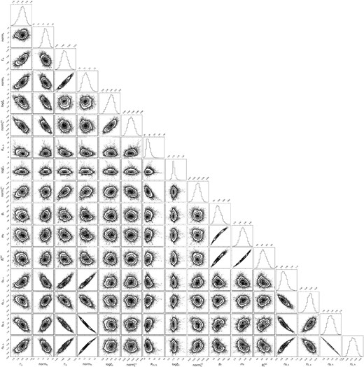
Corner plots for 16 free parameters of the spectral-timing fit in Section 5. Every free parameter has its row and column. The correlation between two free parameters is shown at the intersection of the corresponding row and column. The distribution of each parameter is shown at the rightmost (top) of the corresponding row (column). We use the corner module (Foreman-Mackey 2016) to produce the plots. The figure is viewed clearly in the digital version.
Author notes
Deceased.
