


ABSTRACT
In this paper, we present COMET, a Gaussian process emulator of the galaxy power spectrum multipoles in redshift space. The model predictions are based on one-loop perturbation theory and we consider two alternative descriptions of redshift-space distortions: one that performs a full expansion of the real- to redshift-space mapping, as in recent effective field theory models, and another that preserves the non-perturbative impact of small-scale velocities by means of an effective damping function. The outputs of COMET can be obtained at arbitrary redshifts, for arbitrary fiducial background cosmologies, and for a large parameter space that covers the shape parameters ωc, ωb, and ns, as well as the evolution parameters h, As, ΩK, w0, and wa. This flexibility does not impair COMET’s accuracy, since we exploit an exact degeneracy between the evolution parameters that allows us to train the emulator on a significantly reduced parameter space. While the predictions are sped up by two orders of magnitude, validation tests reveal an accuracy of |$0.1\, {{\ \rm per\ cent}}$| for the monopole and quadrupole (|$0.3\, {{\ \rm per\ cent}}$| for the hexadecapole), or alternatively, better than |$0.25\, \sigma$| for all three multipoles in comparison to statistical uncertainties expected for the Euclid survey with a tenfold increase in volume. We show that these differences translate into shifts in mean posterior values that are at most of the same size, meaning that COMET can be used with the same confidence as the exact underlying models. COMET is a publicly available python package that also provides the tree-level bispectrum multipoles and Gaussian covariance matrices.
1 INTRODUCTION
Models of galaxy clustering statistics inspired by perturbation theory will be one of the main avenues for extracting cosmological information from ongoing and upcoming galaxy surveys, such as the Dark Energy Spectroscopic Instrument (DESI; Levi et al. 2013) and Euclid (Laureijs et al. 2011). That is because on sufficiently large scales, where the validity of the perturbative models can be guaranteed, they reach an unparalleled degree of accuracy, making them a very robust and reliable analysis tool. However, even though perturbative methods have been frequently and successfully used in the analysis of past data sets (e.g. Beutler et al. 2017; Sánchez et al. 2017; Ivanov, Simonović & Zaldarriaga 2020; d’Amico et al. 2020; Semenaite et al. 2022), they cannot be blindly applied to future measurements. The density field associated with each observed population of galaxies will be differently biased with respect to the underlying dark matter field, will have undergone different levels of non-linear evolution, and will be subject to different statistical uncertainties, all of which influence the range of scales on which we can trust the perturbative models. Consequently, each new analysis will need to be accompanied by careful studies of their validity by propagating choices in the modelling, as well as the impact of potential systematics, on to the final results: the cosmological parameters.
Such a task requires running a large number of Monte Carlo Markov Chains (MCMCs) in order to determine the posterior parameter distributions, each of which typically takes of the order |${\cal O}(10^6)$| likelihood evaluations for convergence. Although a single evaluation of the perturbation theory models is comparatively fast, even when performing full-shape fits, and can be executed in |$\sim 1\, \mathrm{s}$| (e.g. Chudaykin et al. 2020; Chen et al. 2021), this still amounts to considerable computational costs. We intend to greatly facilitate this task by constructing an emulator for various clustering statistics in perturbation theory, in particular the multipoles of the redshift-space galaxy power spectrum, that is capable of drastically reducing the time needed for making model predictions (see DeRose et al. 2022; Donald-McCann, Koyama & Beutler 2022, for a similar approach). We thus follow a recent string of works, which introduced emulators as a means of overcoming the much higher computational costs of running simulations, which are needed to extend models of galaxy clustering into the deeply non-linear regime. This enabled efficient modelling of the non-linear matter power spectrum for a set of cosmological parameters (Heitmann et al. 2009; Euclid Collaboration 2019, 2021; Giblin et al. 2019; Angulo et al. 2021), but in combination with a halo occupation distribution model also of the galaxy power spectrum (Kwan et al. 2015; Kobayashi et al. 2020), and the galaxy correlation function in redshift space (Zhai et al. 2019; Yuan et al. 2022). Furthermore, a hybrid approach that makes use of a perturbative expansion of the galaxy bias relation, but obtains all ingredients from simulations was proposed for the galaxy power spectrum in Zennaro et al. (2021), Aricò, Angulo & Zennaro (2021), Kokron et al. (2021), and Pellejero Ibañez et al. (2022). While the accuracy of these emulators is limited by the usually small number of training samples, it is straightforward to build large training sets for models purely based on perturbation theory. Our demand is therefore somewhat different: we want a flexible emulator that covers a large space of model parameters, brings large improvements in computation time and yet does not compromise on the principal advantage of perturbation theory, its accuracy.
In order to satisfy that demand, it is important to keep the parameter space over which the emulator is build as small as possible. As in Donald-McCann et al. (2022) and Aricò et al. (2021), we make use of the fact that all model parameters related to the galaxy bias expansion can be factorized and so their dependence does not need to be emulated. However, what sets our emulator apart from these other works is that it is build around the recently proposed evolution mapping approach (Sánchez et al. 2022), which further limits the emulation parameter space. In this approach, the cosmological parameters are split into two classes: shape parameters, such as the physical baryon and cold dark matter densities, ωb, ωc, and the spectral index ns, and evolution parameters, such as the Hubble parameter |$h \equiv H_0/(100\, \mathrm{km}\, \mathrm{s}^{-1}\, \mathrm{Mpc}^{-1})$|, the scalar amplitude of fluctuations As, the dark energy equation of state parameters, w0, wa, and the curvature density parameter ΩK. At any given redshift, the evolution parameters can only affect the amplitude of the linear matter power spectrum, provided it is expressed in units of Mpc (opposed to the conventional |$h^{-1}\, \mathrm{Mpc}$|), and thus follow an exact degeneracy (Sánchez 2020; Sánchez et al. 2022). Evolution mapping exploits that degeneracy by mapping models with different evolution parameters from one to the other by simply relabelling the redshifts that correspond to the same value of σ12, the RMS of density fluctuations in spheres of radius |$12\, \mathrm{Mpc}$|. We show that this degeneracy extends to the models of perturbation theory considered here, although in redshift-space we additionally need to account for the dependence on the growth rate f. Hence, by training our emulator in terms of σ12 and f in combination with the shape parameters, we can model the effect of the full set of evolution parameters and at arbitrary redshifts. In redshift-space clustering we also need to account for the Alcock-Paczynski (AP) effect (Alcock & Paczynski 1979; Ballinger, Peacock & Heavens 1996a), which requires the assumption of a fiducial background cosmology. We do not include the AP effect in the emulator itself, but in a separate step, and therefore retain more flexibility, which allows us to support any fiducial cosmologies.
This paper is organized as follows. In Section 2, we start by reviewing the perturbative expressions for the galaxy power spectrum multipoles, which our emulator is based on. In particular, we consider two separate models, which differ in their treatment of the real- to redshift-space mapping and show how they can be related. Readers familiar with this material can skip ahead to Section 3, where we describe in detail the evolution mapping approach, as well as further design choices and the computational performance of our emulator. In Section 4, we conduct a series of stringent validation tests of our emulator and propagate any emulation uncertainties on to the posterior distributions of the model parameters, demonstrating no relevant loss in accuracy. We conclude in Section 5 with a comparison to related works and an overview of the capabilities of our python package COMET.
2 OVERVIEW OF PERTURBATION THEORY MODELS
In this work, we consider the emulation of the redshift-space power spectrum multipoles of biased tracers for two different perturbative models. These models differ solely in their treatment of redshift-space distortions with one performing a full expansion of the real-to-redshift space mapping, while the other partly retains the non-perturbative nature of this mapping. Examples of the first category of models are the recent effective field theory (EFT) models of Ivanov et al. (2020) and d’Amico et al. (2020), which introduce a series of counterterms that are meant to capture the effect from small-scale, virialized velocities of galaxies on the power spectrum. Models, such as TNS (Taruya, Nishimichi & Saito 2010) or the one proposed by Sánchez et al. (2017), fall into the second category and account for the virialized velocity impact via an effective damping function that represents the velocity difference generating function (VDG). For the remainder of this paper, we will refer to these two models as EFT and VDG models, respectively.
2.1 Redshift-space power spectra in EFT and VDG models
We note that the VDG model as presented here differs from the TNS model (Taruya et al. 2010) in the effective damping function W∞ and in that the square bracket in equation (10) includes all contributions from quadratic bias, both local and non-local (Sánchez et al. 2017).
2.2 Galaxy bias expansion and stochasticity
In perturbation theory, we predict the clustering of biased tracers, such as dark matter haloes or galaxies, by first relating their overdensities to a series of properties of the underlying dark matter field. This is known as the galaxy bias expansion [see Desjacques, Jeong & Schmidt (2018a) for a comprehensive review], where each property (in the following also denoted as operator) captures an effect of the large-scale environment on the formation and evolution of galaxies, and the strength of that effect is encoded in the associated galaxy bias parameters. While the values of the bias parameters cannot be computed from first principles and also depend on the selection of the observed population of tracers, the various operators to be taken into account at each order of perturbation theory can be derived based on symmetry considerations (McDonald & Roy 2009; Chan, Scoccimarro & Sheth 2012; Assassi et al. 2014; Senatore 2015; Mirbabayi, Schmidt & Zaldarriaga 2015; Desjacques et al. 2018a; Eggemeier, Scoccimarro & Smith 2019).
The last two terms in equation (14) represent the relevant contributions from higher derivative operators and stochasticity, respectively. The former arise when taking into account that gravitational collapse occurs within patches of finite size R, meaning that on distance scales of comparable magnitude, the galaxy overdensity at position |$\boldsymbol{x}$| can no longer be assumed to depend on the matter properties at the same position alone. Expanding this spatial non-locality perturbatively leads to terms scaling as |$\sim R^2\, \nabla ^2 {\cal O}$| with |${\cal O}=\lbrace \delta \, ,\delta ^2\, ,{\cal G}_2\, ,\ldots \rbrace$| (Desjacques 2008; McDonald & Roy 2009; Desjacques et al. 2010, 2018a) and assuming that the scale R is of similar order as the non-linearity scale of the matter field, the term ∇2δ is the only one relevant for the power spectrum at next-to-leading order. Its bias parameter does not appear in the kernels in equations (A9) and (A10), because in Section 2.3 we will absorb it into the definition of one of the counterterms that carries the same scale dependence.
2.3 Definition of counterterms
The loop integrals in equation (8) or equation (12) are performed over the entire range of scales, even those where perturbation can no longer be applied. In order to construct a consistent theory, one needs to introduce a series of counterterms with adjustable amplitudes (i.e. a free parameter per counterterm), which are able to absorb any sensitivity to non-linear modes that might arise in the large-scale limit. It was shown in Senatore & Zaldarriaga (2014) and Desjacques et al. (2018b) that the required leading counterterms for the galaxy power spectrum in redshift-space scale as |$\sim \mu ^{2n}\, k^2\, P_L(k)$| with |$n=0\, ,1\, ,2$|, assuming them for simplicity to be local in time. The first of these scales exactly like the higher derivative bias contribution ∇2δ (see Section 2.2) and so we can absorb its coefficient, |$b_{\nabla ^2\delta }$|, into the corresponding counterterm parameter. The same counterterm also absorbs the leading effect from a breakdown of the perfect fluid approximation for the matter field (Pueblas & Scoccimarro 2009; Baumann et al. 2012; Carrasco, Hertzberg & Senatore 2012). Moreover, Desjacques et al. (2018b) demonstrated that the other two counterterms with n = 1 and n = 2 can account for the relevant velocity bias effects, which we have neglected in our description so far.
2.4 Infrared resummation
The model presented in the previous sections provides a good description of the broadband of the anisotropic galaxy power spectrum on mildly non-linear scales, but exhibits a non-negligible difference in terms of the amplitude of the BAO wiggles (e.g. Baldauf et al. 2015). The latter are most sensitive to large-scale bulk flows, which are responsible for the smearing of the BAO signal via the large-scale relative displacement field.
3 EMULATOR DESIGN
Our emulator is designed around a number of key ideas that minimise the emulation parameter space, while simultaneously keeping the emulator highly flexible, as well as applicable to arbitrary fiducial background cosmologies and a continuous range of redshifts. This is achieved by (1) employing the evolution mapping approach of Sánchez et al. (2022), (2) an exact treatment of Alcock–Paczynski distortions, and (3) a separate emulation of all contributions that are proportional to a unique combination of galaxy bias parameters. In the following, we describe these ideas and further design choices in detail.
3.1 Evolution mapping
3.2 Application of Alcock–Paczynski distortions and VDG damping function
The expression in equation (42) assumes that the power spectrum multipoles are estimated in infinitesimally thin shells k and for a continuous range of μ values. Both of these assumptions are not satisfied for actual measurements, where the multipoles are computed from discrete grids in Fourier space and by averaging over all wave modes that fall into shells of given widths (see e.g. Scoccimarro 2015). As shown in Taruya, Nishimichi & Bernardeau (2013), this leads to sizeable deviations from what equation (42) would predict, in particular for the higher order multipoles and for k values close to the fundamental frequency, kf, of the grid used for the measurements. As described in more detail in Appendix B, one can account for these discreteness effects in the theoretical predictions, which we have implemented as an option in COMET. Up to scales |$k \sim 60\, k_f$|, this comes at no additional computational cost compared to the computation via equation (42).
3.3 Emulated quantities
As is clear from the previous two sections, the task of our emulator is to provide the contributions |$P_{{\cal B}}(\boldsymbol{k}|z)$|. In total, there are 17 different contributions to take into account, summarized in Table 1. For |${\cal B} = b_1$| and |${\cal B}=1$|, we combine linear and one-loop terms, while for |${\cal B} = b_1^2$| we emulate them separately, allowing our emulator to also provide the IR resummed linear power spectrum, which can be useful for other computations. The stochastic contributions (involving the noise parameters |$N^P_0$|, |$N^P_{2,0}$|, and |$N^P_{2,2}$|) do not appear in this list because they do not depend on any cosmological quantities themselves and since we apply AP distortions and the finger-of-god damping separately (see equation 42), we can include them exactly.
Bias contributions to the power spectrum at linear and one-loop order, which scale as PL and |$P_L^2$|, respectively.
| |${\cal B}$| | |$b_1^2$| | b1 | 1 | |$b_1^2$| | |$b_1\, b_2$| | |$b_1\, \gamma _2$| | |$b_1\, \gamma _{21}$| | |$b_2^2$| | |$b_2\, \gamma _2$| | |$\gamma _2^2$| | b2 | γ2 | γ21 | c0 | c2 | c4 | |$b_1^2\, c_{\rm nlo}$| | |$b_1\, c_{\rm nlo}$| | cnlo |
|---|---|---|---|---|---|---|---|---|---|---|---|---|---|---|---|---|---|---|---|
| linear | |$\checkmark$| | |$\checkmark$| | |$\checkmark$| | |$\checkmark$| | |$\checkmark$| | |$\checkmark$| | |$\checkmark$| | |$\checkmark$| | |$\checkmark$| | ||||||||||
| one-loop | |$\checkmark$| | |$\checkmark$| | |$\checkmark$| | |$\checkmark$| | |$\checkmark$| | |$\checkmark$| | |$\checkmark$| | |$\checkmark$| | |$\checkmark$| | |$\checkmark$| | |$\checkmark$| | |$\checkmark$| |
3.3.1 Projection into multipoles and reconstruction of anisotropic power spectrum
3.3.2 Constructing ratios with the linear power spectrum
3.3.3 Summary
In summary, we thus require an emulation of the following quantities:
|$\beta _{{\cal B},\ell }(k|\boldsymbol{\Theta }_{\rm s},\sigma _{12},f)$| for ℓ = 0, 2, 4, and each |${\cal B}$| from Table 1 ,
|$P_L\left(k|z=1,\boldsymbol{\Theta }_{\rm s},\boldsymbol{\Theta }_{\rm e}^{\rm fixed}\right)$| ,
|$\sigma _{12}\left(z=1,\boldsymbol{\Theta }_{\rm s},\boldsymbol{\Theta }_{\rm e}^{\rm fixed}\right)$| ,
|$\sigma _{v}\left(z=1,\boldsymbol{\Theta }_{\rm s},\boldsymbol{\Theta }_{\rm e}^{\rm fixed}\right)$| .
We evaluate the ratios and PL on a range of scales extending from |$7 \times 10^{-4}\, \mathrm{Mpc}^{-1}$| to |$0.35\, \mathrm{Mpc}^{-1}$|, using a total number of 106 points, chosen such that they provide a dense sampling on scales relevant for the BAO wiggles.
3.4 Parameter space and training process
3.4.1 Parameter ranges
Our emulator is constructed for a total of five parameters. In addition to f and σ12, we consider the three shape parameters ωb, ωc, and ns. Each of them is allowed to vary within the ranges given in Table 2, which for the latter three were chosen to span roughly a 12, 30, and 11σ interval around the Planck 2018 best-fitting values, respectively. The growth rate and σ12 capture the dependence on redshift and an arbitrary set of evolution parameters,8 and therefore require a more generous support. None the less, the limits on f and σ12 impose restrictions on the range of redshifts for which our emulator can be used. In case of the growth rate the ranges can accommodate any redshift for ωc ≳ 0.107, while for the most extreme values of the allowed shape parameters the lower boundary imposes the limitation z ≳ 0.1. Tighter restrictions on the supported redshifts come from the range of σ12 and to demonstrate that we compare them in Fig. 1 against the Planck prediction of σ12 as a function of redshift using the best-fitting cosmological parameter values from Planck Collaboration VI (2020). When exploring cosmological parameters using a large-scale structure likelihood function, they will give rise to values of σ12 that are typically close (within |$\sim 10\, {{\ \rm per\ cent}}$|) to the Planck prediction, while the 1σ uncertainty on σ12 is of the order |$5\, {{\ \rm per\ cent}}$| for constraints from the BOSS galaxy survey (Semenaite et al. 2022). To account for these uncertainties, we plot a 20 per cent error band around the Planck prediction in Fig. 1 and expect that any sampled cosmological parameters will correspond to σ12 values falling roughly into that range. We see that this band leaves the σ12 range of our emulator at a redshift z ∼ 3, which means that COMET is no longer guaranteed to provide accurate predictions beyond that redshift.
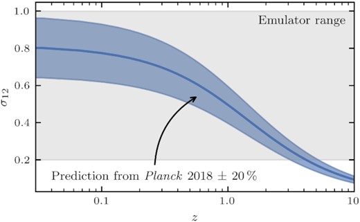
Prediction of σ12 as a function of redshift using the Planck 2018 TT, TE, EE + lowE + lensing best-fitting cosmological parameters. The blue-shaded band represents a 20 per cent variation around that prediction, while for comparison the supported range of values for σ12 in our emulator COMET is shown as the grey-shaded area.
Emulator parameter space and the supported range of values.
| Parameter | Min. emulator range | Max. emulator range |
|---|---|---|
| ωb | 0.0205 | 0.02415 |
| ωc | 0.085 | 0.155 |
| ns | 0.92 | 1.01 |
| σ12 | 0.2 | 1.0 |
| f | 0.5 | 1.05 |
| Parameter | Min. emulator range | Max. emulator range |
|---|---|---|
| ωb | 0.0205 | 0.02415 |
| ωc | 0.085 | 0.155 |
| ns | 0.92 | 1.01 |
| σ12 | 0.2 | 1.0 |
| f | 0.5 | 1.05 |
3.4.2 Generation of training data sets
We generate two separate training sets, one spanning the full parameter space intended for the ratios |$\beta _{{\cal B},\ell }$|, and another covering only the shape parameters for the remaining quantities. Both training sets are built by drawing a number of samples from a Latin Hypercube, using 1500 and 750 samples, respectively. In order to obtain an optimal coverage of the parameter spaces we repeat the sampling step 10 000 times and pick the set which maximizes the minimum (Euclidean) distance between any two of its points. We then evaluate all of the model ingredients using a numerical integrator and starting from camb-generated linear input power spectra. Before training the emulator, we perform one additional pre-processing step, in which we further reduce the dynamical range of the training data by taking the logarithm and in which we normalize each component, such that it has zero mean and unit variance over the full set of samples.
3.4.3 Gaussian process emulation
3.5 Computational performance
In this section, we measure the execution times of COMET for the two different RSD models, each for a different number of multipoles and number of scales. The computational performance will of course depend on the given platform, so the reader should keep in mind that all measurements reported here are based on a laptop equipped with an Apple M1 Pro processor, using one CPU (up to 3.22 Ghz) and a single thread.
We measure the execution times using the function perf_counter from python’s time module and in order to reduce uncertainties, we repeat the prediction of the power spectrum multipoles Nexec times for values of Nexec ranging from 1 to 35. We then fit a straight line to the resulting measurements as a function of Nexec, such that the slope of that line provides a robust estimate (and uncertainty) of the execution time per call. In Fig. 2, we plot these estimates for a varying number of scales spaced logarithmically between |$k_{\rm min} = 0.001\, \mathrm{Mpc}^{-1}$| and |$k_{\rm max} = 0.35\, \mathrm{Mpc}^{-1}$| for the EFT model in blue and the VDG model in orange. Filled symbols in each case correspond to the prediction of only the monopole, while open symbols also include the computation of the quadrupole and hexadecapole. We see that the execution times range from |$\sim 9.5\, \mathrm{ms}$| to |$\sim 11.5\, \mathrm{ms}$| for 50–300 bins in case of the EFT model. The VDG model takes on average about |$1\, \mathrm{ms}$| longer, due to the integration over μ also involving the evaluation of the effective damping function W∞. On the other hand, we see little difference between a prediction of just the monopole, or all three multipoles, since for the reconstruction of the anisotropic power spectrum the emulator of all three multipoles need to be called in any case.
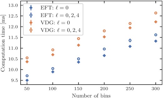
Computation time as a function of the provided number of bins for the EFT and VDG models, either for the monopole alone, or all three multipoles.
Considering that the execution time for other public codes, such as CLASS-PT (Chudaykin et al. 2020) or PyBird (D’Amico, Senatore & Zhang 2021) is of the order |$\sim 1\, \mathrm{s}$| (based on a timing estimate given by the authors of the former code, but using more than one CPU), COMET achieves a speed-up of at least two orders of magnitude.
4 VALIDATION OF THE EMULATOR
In this section, we perform a number of mock analyses based on synthetic data sets at multiple redshifts using statistical uncertainties corresponding to a volume ten times larger than that expected for the Euclid galaxy survey. These analyses not only allow us to determine the relative uncertainties introduced by the emulator, they also – and this is of much greater relevance – let us test how these uncertainties propagate to the posteriors of cosmological and galaxy bias parameters.
4.1 Generation of synthetic validation data
4.1.1 ΛCDM validation set
Our main validation sample consists of a set of flat ΛCDM cosmologies covering the parameters ωb, ωc, ns, h, and As for the EFT model, while for the VDG model we also include avir. Each validation set is generated by drawing 1500 random points within these five-, or six-dimensional parameter spaces, satisfying only the minimum and maximum values given in Table 3. For each point in the validation set, we compute the power spectrum multipoles using the exact model at the four redshifts z = 0.9, 1.2, 1.5, and 1.8, and making the following assumptions for the galaxy bias parameters: we fix the value of the linear bias using |$b_1(z) = \sqrt{1+z}$|, which provides a reasonable estimate of the bias of H α galaxies to be selected by Euclid (Rassat et al. 2008; di Porto, Amendola & Branchini 2012), whereas for γ2 we impose the excursion-set relation of Sheth, Chan & Scoccimarro (2013) and Eggemeier et al. (2020). We then determine the values of b2 and γ21 according to the peak-background-split and coevolution relations from Lazeyras et al. (2016) and Eggemeier et al. (2019), respectively, as functions of b1 and γ2, and set all other counterterm and stochastic model parameters to zero. Each of the synthetic multipoles accounts for Alcock-Paczynski distortions in an exact manner (i.e. not via the approximation discussed in Section 3.3.1), based on a fiducial flat ΛCDM cosmology at the same redshifts as the predictions and with fixed parameters h = 0.67 and ωm = ωc + ωb = 0.1432.
Parameters included in the ΛCDM validation set and their minimum and maximum values. The parameter avir is only included in the validation set for the VDG model and its minimum and maximum values are given in units of |$h^{-1}\, \mathrm{Mpc}$|.
| Parameter | Minimum | Maximum |
|---|---|---|
| ωb | 0.02100 | 0.02365 |
| ωc | 0.095 | 0.145 |
| ns | 0.93 | 1.00 |
| h | 0.55 | 0.85 |
| As | 0.8 | 3.0 |
| avir | 0.0 | 8.0 |
| Parameter | Minimum | Maximum |
|---|---|---|
| ωb | 0.02100 | 0.02365 |
| ωc | 0.095 | 0.145 |
| ns | 0.93 | 1.00 |
| h | 0.55 | 0.85 |
| As | 0.8 | 3.0 |
| avir | 0.0 | 8.0 |
In a second step, we construct statistical uncertainties for these synthetic measurements by adopting Gaussian covariances matrices, which are computed from the synthetic multipoles at each point in the validation set using the expressions given, for instance, in Grieb et al. (2016). In order to relate these uncertainties to the characteristics of the Euclid survey, we further assume tracer densities that match the number densities of H α galaxies in the Euclid Flagship I mock catalogues (see Table C1), as well as Euclid-like volumes. The latter are derived from redshift shells of width Δz = 0.2, centred on the respective redshifts for which the power spectrum multipoles have been evaluated, and covering a sky area of |$15\,000\, \mathrm{deg}^2$|. To increase the stringency of our validation tests, we then multiply these volumes by a factor of 10, which is equivalent with a reduction of the statistical uncertainties by a factor of ∼3.
We stress that the various choices in generating this synthetic data set are not meant to provide power spectrum measurements that closely mimic those of any real galaxy samples. Nonetheless, we expect the relative uncertainties, σℓ/Pℓ, to be well representative (apart from the stringency volume factor) for Euclid, such that we can make a meaningful assessment of the performance of our emulator.
4.1.2 Synthetic measurements for fixed set of parameters
For a further validation test we generate one more set of synthetic power spectrum multipoles at fixed cosmological and bias parameters. We compute the power spectrum multipoles from the exact model (in this case only for the EFT) at the same four redshifts as before, but using the bias parameter values for b1, b2, γ21, c0, c2, c4, cnlo, and |$N^P_0$| given in Table C1. The value for γ2 is again fixed in terms of the excursion set relation, while the cosmological parameters at all four redshifts are set to h = 0.67, ωc = 0.1212, ωb = 0.021996, ns = 0.96, and As = 2.11065. As described in Section 4.1.1, we then derive statistical uncertainties for these synthetic measurements in the Gaussian approximation, using the number densities specified in Table C1 and volumes that correspond to the same redshift shells as above, including the stringency factor of 10.
4.2 Results across ΛCDM validation set
Our goal is to quantify the impact of the emulation inaccuracies on mean parameter values and their uncertainties, when performing a full likelihood exploration using all three galaxy power spectrum multipoles. To that end we use the synthetic data vectors and covariance matrices described in Section 4.1.1 and for each combination of cosmological parameters in the validation set we run two MCMC,9 one with the exact theory model, the other using the emulator predictions. In those chains, we keep the cosmological parameters fixed, while varying a set of seven bias parameters: b1, b2, γ21, the constant shot noise N0, as well as the three counterterm parameters c0, c2, and c4; γ2 is fixed in terms of the aforementioned excursion set relation as a function of b1. We pick a maximum wavemode of |$0.3\, h\, \mathrm{Mpc}^{-1}$| for all three multipoles in this analysis, which means that any significant deviations between the true and emulated models up to that scale can lead to shifts between the posterior mean values recovered from the two chains, as well as to differences in the credible regions.
4.2.1 Relative inaccuracies
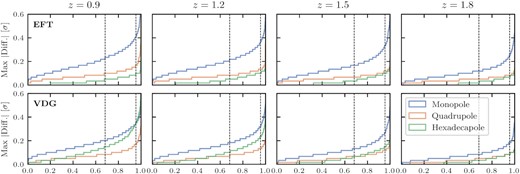
Before identifying the effects on the parameter constraints, let us first consider the relative differences between the exact model and the emulator as a function of scale. These are shown exemplarily for the EFT model at z = 0.9 in the upper panels of Fig. 3, where each line has been evaluated for a different point in the validation set and a randomly selected point from the chain over bias parameters that was run for the exact model. We see that the relative differences for the monopole (blue) and quadrupole (orange) grow between |$k = 0.1\, h\, \mathrm{Mpc}^{-1}$| and |$0.2\, h\, \mathrm{Mpc}^{-1}$|, after which they saturate and generally stay below the |$0.2\, {{\ \rm per\ cent}}$| threshold. This can be seen more clearly in the cumulative histogram in the fourth panel, which plots the maximum of the absolute relative difference over all scales and shows that there is only a vanishingly small fraction of cosmologies in the validation data sets that gives rise to discrepancies larger than |$0.2\, {{\ \rm per\ cent}}$|. In fact, we find that |$68\, {{\ \rm per\ cent}}$| of all validation samples have maximum uncertainties smaller than |$0.08\, {{\ \rm per\ cent}}$| and |$0.1\, {{\ \rm per\ cent}}$| for the monopole and quadrupole, respectively. The situation is slightly worse for the hexadecapole, where for the same fraction of validation samples the maximum differences are only below |$0.3\, {{\ \rm per\ cent}}$|, but this is mostly due to the hexadecapole crossing zero for many of the tested cosmologies. It is more meaningful to plot these differences in units of some estimate of the measurement uncertainties, and for the results in the lower panels of Fig. 3 we have picked the standard deviations taken from the covariance matrices discussed in Section 4.1.1. We now obtain the reversed picture: due to the monopole having the smallest uncertainties, its differences appear larger than for both, the quadrupole and hexadecapole, so it will dominate the impact on any parameter posteriors. However, |$68\, {{\ \rm per\ cent}}$| of the validation samples still have a maximum difference smaller than |$0.24\, \sigma$| at 10 times the Euclid volume for this redshift shell. The analogous results for the VDG model and the other redshifts are qualitatively very similar – we only note that the differences in units of the measurement uncertainties decrease with increasing redshift because of the decreasing tracer number densities and thus a larger contribution from shot noise (see Appendix C).
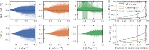
Inaccuracies of the emulated multipoles as a function of scale for the EFT model at z = 0.9. Differences are shown in per cent (upper panels) and in units of the standard deviation of our synthetic data set (covering 10 times the volume of a Euclid redshift shell, see Section 4.1.1; lower panels) for all cosmologies of the validation set and using a combination of bias parameters from a random point in each chain. The fourth panel shows the cumulative histogram of the maximum absolute differences over the full range of scales with the two vertical dashed lines indicating |$68\, {{\ \rm per\ cent}}$| and |$95\, {{\ \rm per\ cent}}$| of the validation samples.
4.2.2 Shifts in posterior means
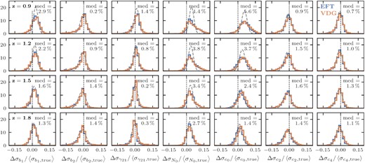
In order to study, the impact of these inaccuracies on the parameter posteriors, we extract the 1D-marginalized posterior means for each of the seven bias parameters from the two chains and compute their difference in units of the 1σ parameter uncertainty obtained from the chain using the exact model, σX, true (with X denoting any of the seven bias parameters). Fig. 4 shows the resulting histograms over the full validation set for all four redshifts and both of the RSD models. We clearly see that none of these cases produces any significant shifts in the varied parameters. More precisely, the means of the distributions stay consistently below |$0.1\, \sigma _{X,\mathrm{true}}$|, while the standard deviations reach a maximum of |$0.2\, \sigma _{X,\mathrm{true}}$|, showing that for the majority of the validation cosmologies we recover the true posterior means with high accuracy, while even the largest shifts remain negligible for the nominal Euclid volume. The parameters b1 and N0 generally display the smallest shifts, since they already get well constrained by the large-scale power spectrum, where the emulation inaccuracies are smallest. The higher order bias parameters b2 and γ21, as well as the counterterm parameters, on the other hand, are mostly constrained from the non-linear regime, such that they are more susceptible to the slightly larger emulation errors for k-modes beyond |$0.2\, h\, \mathrm{Mpc}^{-1}$|. The largest shift (with a mean value of |$\sim 0.25\, \sigma _{X,\mathrm{true}}$|) occurs for c4 in case of the VDG model at z = 0.9. As we will show in Section 4.4, this is because the VDG model is more heavily affected by inaccuracies from the reconstruction of the anisotropic power spectrum and these inaccuracies are most notable for the small-scale hexadecapole. Since c4 is mainly constrained by the hexadecapole, it absorbs these mismatches, resulting in the larger shifts. Finally, we note that the standard deviations for the distributions of the shifts are a little smaller than the value of the maximum difference (in units of σ) for |$68\, {{\ \rm per\ cent}}$| of the samples found in Section 4.2.1, but they are generally consistent, suggesting that the latter can serve as a good indicator for the performance of the emulator in explorations of the likelihood.
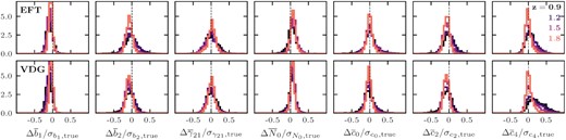
Distributions of the differences between the posterior mean values obtained from running MCMC with the exact and emulated model predictions. Chains were run for synthetic data including the monopole, quadrupole and hexadecapole up to |$k_{\rm max} = 0.3\, h\, \mathrm{Mpc}^{-1}$| with uncertainties corresponding to expected errors for the Euclid survey (see Section 4.1.1), but with ten times larger volumes. Each column shows the distribution for a different parameter varied in the chain in units of the respective standard deviation extracted from the chain using the true model, while the two different rows correspond to the different RSD models. The transition from dark to bright colours indicates increasing redshifts.
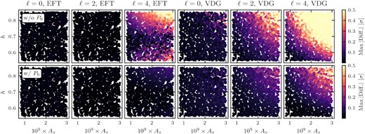
It is instructive to check whether the largest inaccuracies from the emulator occur dominantly in certain parts of the cosmological parameter space. For that reason in Figs 5 and 6, we plot the shifts in the linear bias parameter for the EFT and VDG models at z = 0.9, respectively, using all two-dimensional projections of the validation parameter set. We see indeed that for certain parameter combinations larger shifts (lighter colours) do not appear randomly, but in well separated regions: for instance, for the EFT model the most obvious separation occurs in the ωb–ωc parameter plane, showing that there are larger inaccuracies for large values of ωb and simultaneously small values of ωc. A similar trend can also be observed for the VDG model, in which case there is an additional tendency for larger shifts in the ωb–As parameter plane. We obtain similar results for the other redshifts, emphasizing that in central regions of the parameter space, in particular for values of ωb close to the Planck or Big Bang Nucleosynthesis priors, where one would preferentially sample the cosmological likelihood, the emulator performs best.
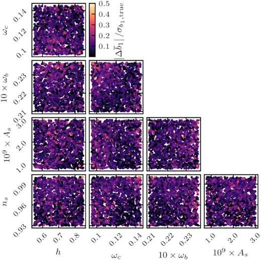
Shifts in the posterior means of b1 between the true and emulated EFT model at z = 0.9. Each panel shows a scatter plot of all validation samples, projected into different parameter planes.
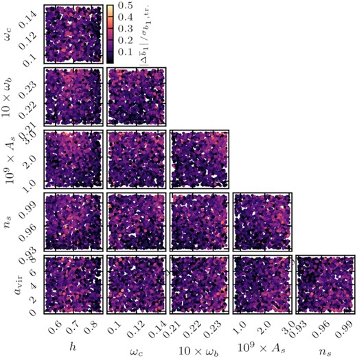
Same as Fig. 5, but for the VDG model at z = 0.9.
4.2.3 Impact on credible regions
Finally, let us consider how well we can recover the 1σ credible regions for the parameters varied in the chains. This is more difficult to quantify precisely because, unlike the posterior means, the credible regions are more heavily affected by sampling noise, i.e. they carry a stronger dependence on the initial seed used for the MCMC at fixed convergence criterion. Ideally, we would therefore first quantify the sampling noise for each point in the validation set by running multiple chains with different initial seeds and constructing probability distributions of the 1σ credible region for each parameter, which could be compared between the exact and emulated models. However, as that procedure is very costly due to the need of running many individual chains, we settle on an approximate comparison only.
First we assume that the sampling noise is independent of cosmology and that the values of the 1σ confidence limits for each bias parameter are drawn from Gaussian distributions with means |$\overline{\sigma }_{X,\mathrm{true/emu}}(\boldsymbol{\Theta })$| and variance |$\sigma _{X, \mathrm{sampling}}^2$|, where |$\boldsymbol{\Theta }$| denotes the dependence on cosmological parameters contained in the validation set. The difference in the estimated 1σ confidence limits between the true and emulated models is then also Gaussian distributed with mean |$\overline{\sigma }_{X,\mathrm{emu}}(\boldsymbol{\Theta }) - \overline{\sigma }_{X,\mathrm{true}}(\boldsymbol{\Theta }) = \Delta \overline{\sigma }_{X}(\boldsymbol{\Theta })$| and variance |$2\sigma ^2_{X,\mathrm{sampling}}$|. In the case that |$\Delta \overline{\sigma }_X(\boldsymbol{\Theta })$| is small or has negligible dependence on cosmology, we can regard each value ΔσX obtained at a different validation cosmology as being independently drawn from the same sampling noise distribution and we can interpret the offset of that distribution from zero mean as the accuracy with which we can recover the 1σ credible regions. On the other hand, if |$\Delta \overline{\sigma }_X(\boldsymbol{\Theta })$| strongly depends on cosmology, the distribution of ΔσX values over the validation set will be broader and/or have a different shape, and so we cannot immediately assess the significance of the differences in σX from the data we have generated.
In Fig. 7, we plot the distributions of ΔσX, normalized by the average over the entire validation set, <σX, true >, for the two RSD models and the four different redshifts. In order to quantify the sampling noise, we pick a ΛCDM cosmology with parameter values corresponding to the Planck 2018 TT, TE, EE + low E + lensing constraints, for which we run 1000 chains with the exact predictions for the EFT and VDG models at each redshift, and varying the same seven bias parameters as before, but with different initial seeds. We then determine |$\sigma ^2_{X,\mathrm{sampling}}$| in each case by fitting a Gaussian to the resulting distributions of σX/ < σX > −1, where <σX > is the average of σX over the 1000 different chains. This allows us to plot the reference sampling noise distributions (grey dashed lines in Fig. 7) as Gaussians with variance |$2\sigma _{X,\mathrm{sampling}}^2$| and mean given by the median of the EFT distributions (blue histograms).
Histograms of the differences in the |$68\, {{\ \rm per\ cent}}$| credible regions between the true and emulated models, normalized by the average 1σ constraints obtained from the true model of all validation samples, <σX, true >. Each column depicts a different parameter varied in the chains, while each row shows a different redshift of the synthetic data set; the two different colours correspond to the two RSD models. The grey dashed lines are Gaussian distributions, centred on the median value of the EFT histograms, and represent an estimate of the spread due to sampling noise alone (see the text for details).
From these plots, we observe that many of the histograms over the validation set are indeed consistent with sampling noise and moreover, in those cases the differences between σX, true and σX, emu are at the per cent level, which is insignificant compared to the spread due to sampling noise. Some parameters, in particular b1, N0, and c0, display broader or skewed distributions, suggesting that in those cases the cosmology dependence of the differences of σX is stronger. In those cases, we can only deduce that on average the differences are still at the per cent level (see median values), but it is not possible to judge their significance. The deviations from the sampling noise distributions are largest at z = 0.9, where the synthethic measurements uncertainties are smallest and hence where the emulation inaccuracies carry the strongest weight, while going to z = 1.8 gives again very good consistency with sampling noise for all parameters. We do not find any significant differences between the two RSD models.
4.3 Results for analysis with varying cosmological parameters
Finally, we analyse the synthetic power spectrum multipoles described in Section 4.1.2. As before, we run two chains, one with the exact model, the other using COMET, but instead of keeping the cosmological parameters fixed as in the previous section, we now also vary h, ωc, and As, setting only ns and ωb to their fiducial values. Out of the full set of bias parameters we include b1, b2, γ21, c0, c2, c4, and N0 in the chains, fixing γ2 and cnlo to the values used in the generation of the synthetic data. Since explorations of the likelihood with varying cosmological parameters is much more computationally expensive for our exact model code, we limits ourselves here to only a single case per redshift.
The chains are run using MultiNest (Feroz & Hobson 2008; Feroz, Hobson & Bridges 2009; Feroz et al. 2019) with 1800 live points in case of COMET and a standard Metropolis–Hastings sampler with a total number of 42 000 accepted steps in case of the exact model. After processing these chains with getdist (Lewis 2019) we obtain the 2d marginalized posteriors for the full set of parameters at redshift z = 0.9 shown in Fig. 8, where the results based on the exact model correspond to the blue contours, the ones based on COMET to the orange contours. We see that the agreement between the posteriors of the two models is close to perfect: the mean posterior values of all parameters are almost identical and any occurring shifts are well below the 1σ level, while the 1σ and 2σ credible regions are equally well recovered. Some slight differences can be observed in the tails of the posterior distributions, but these are most sensitive to the sampling routines and therefore most likely caused by differences in the two samplers used here. Although not shown, we find qualitatively very similar results at the three remaining redshifts, so that these findings confirm our results from Section 4.2 at fixed cosmology.
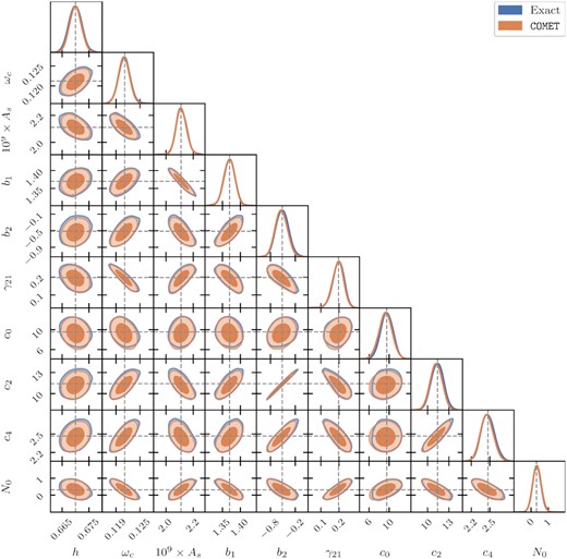
Comparison of the 2d and 1d marginalized posteriors obtained from running MCMC with the exact model and COMET for the EFT. The results shown stem from the synthetic data set at redshift z = 0.9, as described in Section 4.1.2 and using a volume corresponding to 10 times the volume of a Euclid redshift shell. The value of γ2 was constrained to the excursion set relation of Eggemeier et al. (2020), while cnlo was fixed to the fiducial value (see Table C1). The three counterterm parameters c0, c2, and c4 are given in units of |$(h^{-1}\, \mathrm{Mpc})^2$|. Vertical and horizontal dashed lines indicate the fiducial parameter values.
4.4 Reconstruction of anisotropic power spectrum
In this section, we report the impact of inaccuracies caused by reconstructing the full anisotropic power spectrum from the monopole, quadrupole, and hexadecapole only, as well as the approximate inclusion of the ℓ = 6 multipole discussed in Section 3.3.1. To that end we make again use of the validation set described in Section 4.1.1 and compute the first three multipoles for each validation cosmology using the exact model (i.e. without any input from the emulator), but without inclusion of Alcock–Paczynski distortions and, in case of the VDG model, without the FoG damping term. Like for our emulator, we then reconstruct the anisotropic power spectrum from those multipole moments, apply Alcock–Pacyznski distortions and FoG damping, and as a final step evaluate the observed multipoles. We can compare these predictions with those that do not make use of the multipole reconstruction in order to determine the differences as a function of the cosmological parameters.
This is shown in the top row of Fig. 9, where we plot the maximum difference (taken over all scales up to |$k_{\mathrm{max}} = 0.3\, h\, \mathrm{Mpc}^{-1}$|) in units of the synthetic standard deviations for each validation point at z = 0.9, projected into the h–As parameter plane. The first three panels depict these differences for the monopole to hexadecapole for EFT model, the next three for the VDG model. We note that for the EFT model there is virtually no impact on the monopole and quadrupole, even for measurement uncertainties corresponding to 10 times the volume contained in a Euclid redshift shell. The situation is different for the hexadecapole, where we obtain maximum differences of up to ∼0.5σ, in particular for large and small values of h. On the other hand, for the VDG model the effect is noticeably larger with maximum differences going well beyond 0.5σ for the hexadecapole (up to ∼2.5σ) and also more significant inaccuracies for the monopole and quadrupole, preferentially for large values of h and As. This happens because the FoG damping factor carries a significant additional line-of-sight dependence, which amplifies the contributions from higher multipole moments not included in the reconstruction.
Maximum differences up to |$k_{\mathrm{max}} = 0.3\, h\, \mathrm{Mpc}^{-1}$| (in units of the standard deviation of our synthetic data set, see Section 4.1) for each point of the validation set between the exact computation of the power spectrum multipoles and when the anisotropic power spectrum before application of Alcock-Paczynski distortions and FoG damping is obtained from a Legendre decomposition truncated at finite order. In the top row the latter is based on the first three non-zero multipoles, while in the bottom row we include the ℓ = 6 multipole moment evaluated at fixed shape parameters (see Section 3.3.1 for details). Both sets of predictions are generated without any input from the emulator.
The lower panels of Fig. 9 shows how the maximum difference improve when the ℓ = 6 multipole, evaluated at fixed shape parameters corresponding to the Planck 2018 TT,TE,EE+lowE + lensing values, is included in the Legendre expansion. We see that even when using this approximation the inaccuracies are significantly reduced for both RSD models. Specifically, they now stay below ∼0.2σ for the hexadecapole of the EFT model, while only about |$5\, {{\ \rm per\ cent}}$| of the validation samples reach maximum difference larger than ∼0.2σ and 0.35σ for the quadrupole and hexadecapole of the VDG model, respectively. Returning to the larger shifts in the counterterm parameter c4 that we noticed in Section 4.2.2 for the VDG model, we find that they depend on cosmology in a very similar way as the differences in the bottom right panel of Fig. 9, implying that these shifts are caused by the remaining reconstruction inaccuracies in the hexadecapole. However, we stress that these are not only negligible, they also occur in a region of the cosmology parameter space that is not relevant for likelihood explorations.
5 CONCLUSIONS
5.1 Summary
We have presented COMET, an emulator of the galaxy power spectrum multipoles in redshift-space based on two different perturbation theory models: the EFT model as employed in the analyses of Ivanov et al. (2020), d’Amico et al. (2020), which fully expands the real- to redshift-space mapping, and the VDG model, which models the impact of small-scale velocity differences via a non-perturbative damping function (Scoccimarro 2004; Taruya et al. 2010; Sánchez et al. 2017). The leading idea that was driving the design of our emulator was to minimise the emulation parameter space, in order to reach an optimal compromise between computation time and accuracy. For that reason we have adopted the evolution mapping approach of Sánchez et al. (2022) and trained COMET internally in units of Mpc over the range |$0.0007\, \mathrm{Mpc}^{-1}$| to |$0.35\, \mathrm{Mpc}^{-1}$| using only the shape parameters ωb, ωc, ns, in addition to σ12 and the growth rate f. In this way we are able to support a broad set of evolution parameters, specifically h, As, ΩK, w0, and wa, by mapping them to the corresponding values of σ12 and f at any given redshift (up to an upper limit of z ∼ 3, imposed by our chosen range for σ12). Furthermore, we emulate all independent contributions that arise from the galaxy bias expansion separately, which precludes the associated parameters from the emulator parameter space, and apply AP distortions and the effective damping function in case of the VDG model in a separate step. This gives COMET the flexibility to support any fiducial background cosmologies and arbitrary functional forms of the damping term. A single evaluation of the monopole, quadrupole and hexadecapole at |${\cal O}(100)$| scales takes about |$10\, \mathrm{ms}$| when executed on a single CPU.
Using a series of validation tests, we verified that COMET does not introduce any relevant loss in accuracy in comparison to the exact perturbation theory models. We constructed a large validation set consisting of 1500 synthetic power spectrum measurements at four different redshifts between z = 0.9 and z = 1.8, covering the five-dimensional cosmological parameter space: ωb, ωc, ns, h and As. Adopting a fixed set of galaxy bias parameters at each redshift and in case of the EFT model, we find that the relative inaccuracies stay below |$0.08(0.14)\, {{\ \rm per\ cent}}$|, |$0.11(0.17)\, {{\ \rm per\ cent}}$| and |$0.30(1.33)\, {{\ \rm per\ cent}}$| for |$68(95)\, {{\ \rm per\ cent}}$| of the validation samples and the monopole, quadrupole, and hexadecapole, respectively, up to |$k_{\rm max} = 0.3\, h\, \mathrm{Mpc}^{-1}$|. We further generated statistical uncertainties for our synthetic measurements using Gaussian covariances and specifics tied to the Euclid survey, but with a tenfold increase in volume. In units of these uncertainties the emulation errors are below |$0.24(0.42)\, \sigma$|, |$0.10(0.17)\, \sigma$|, and |$0.05(0.10)\, \sigma$|. We then ran MCMC, varying a set of seven bias parameters both for COMET and the exact model and analysing all three synthetic multipoles for each validation sample, finding that the shifts in the mean posterior values closely match the emulation inaccuracies in units of σ. Additionally, we find that the |$68\, {{\ \rm per\ cent}}$| credible regions are very well recovered and any occurring differences are typically smaller than the MCMC sampling noise. For the VDG model the performance is very similar, apart from a slightly less accurate hexadecapole (see discussion in Section 4.4), but without negative effects on the recovery of the posteriors. Finally, we constructed one more synthetic collection of measurements (again at the same four redshifts) for a fixed set of cosmological and bias parameters, which we used to demonstrate that even when running chains over the full parameter space (including cosmological parameters) there is no appreciable difference in the resulting posterior distributions between the exact model and COMET.
While we have explicitly demonstrated that the emulator is accurate up to scales of at least |$k_{\rm max} = 0.3\, h\, \mathrm{Mpc}^{-1}$|, we caution that this does not have to apply to the underlying theoretical model itself. The validity of the one-loop perturbation theory depends on the relative size of the neglected non-linear corrections, as well as the amplitude of the galaxy bias parameters, and is thus a function of redshift and the particular galaxy sample under consideration. Any application to real data must therefore be preceded by a thorough study of the model’s robustness under changes of the maximum scale cuts — a task that is ideally suited for COMET due to its superior computational efficiency.
We leave two important extensions of COMET to forthcoming publications: Firstly, the power spectrum models for both the EFT and VDG can be easily transformed to configuration space and thus, using the same emulation technniques as presented here, we would also be able to make fast predictions of the two-point correlation function multipoles. Secondly, the new generation of galaxy surveys is expected to improve our current constraints on the masses of neutrinos, which is why it is particularly important to be able to predict galaxy clustering statistics as a function of non-zero neutrino masses, unlike we have assumed here.
5.2 Comparison to related emulators in the literature
While most galaxy clustering emulators that have been presented in the literature so far have been built from simulations and focus on the non-linear regime, there are two sets of works, which are closely related to what we have presented here and which we want to briefly compare against. In particular, Donald-McCann et al. (2022), DeRose et al. (2022) have presented two perturbation theory emulators of the galaxy power spectrum multipoles. The former, EFTEMU, is based on the PyBird code (d’Amico et al. 2020), which implements perturbation theory expressions identical to those described in Section 2 for the EFT model apart from slight differences in the infrared resummation procedure10 and the definition of the galaxy bias parameters (see Section 2.2 for a conversion), while the latter, EmulateLSS, is based on the Lagrangian perturbation theory model of Chen et al. (2021). Although sharing the same goal, there are a number of differences between these two emulators and COMET. On the one hand, this concerns the parameter space and the range of scales for which they provide predictions: EFTEMU supports the five cosmological parameters ωb, ωc, h, As, and ns (i.e. it does not allow for deviations from the equation of state of a cosmological constant or for non-flat cosmologies), and with the exception of ns all of these have smaller ranges than in COMET. EmulateLSS is even more restrictive as it also fixes the spectral index and does not cover the full galaxy bias and counterterm parameter space, ignoring for instance the second- and third-order tidal bias parameters. Moreover, both of these emulators make predictions for a fixed fiducial background cosmology and at fixed redshifts (each new fiducial background cosmology or redshift would require generating a new set of training data) and while EmulateLSS gives predictions in the range of scales from |$0.001\, h\, \mathrm{Mpc}^{-1}$| to |$0.5\, h\, \mathrm{Mpc}^{-1}$|, EFTEMU has a more limiting range with a maximum wavemode of |$0.19\, h\, \mathrm{Mpc}^{-1}$|. On the other hand, the prediction accuracies for the three multipoles quoted by DeRose et al. (2022) are only slightly worse than what we have determined for COMET, and also Donald-McCann et al. (2022) find a sub-per cent accuracy for fixed BOSS-like galaxy bias parameters, making it comparable with COMETin this regard (albeit on a more limited range of scales). Finally, both EFTEMU and EmulateLSS use neural networks instead of Gaussian processes for the emulation procedure and their computation time therefore does not depend on the size of the training set. This leads to a better computational performance than COMET by about one order of magnitude based on the fact that both works quote a computation time of |$\sim 1\, \mathrm{ms}$| (we stress, however, that eventually the computational bottleneck will lie elsewhere, e.g. in the computation of the χ2 or, for joint chains with the bispectrum, the computation of the bispectrum model).
The methodology discussed in Zennaro et al. (2021), Aricò et al. (2021), and Kokron et al. (2021) follows the same perturbative galaxy bias expansion as presented in Section 2.2 (although the third order term related to the parameter γ21 is neglected) and they have presented emulators for the various contributions to the galaxy power spectrum based on either perturbation theory (Aricò et al. 2021) like here, or on simulations in order to extend the predictions into the non-linear regime (Zennaro et al. 2021; Kokron et al. 2021). All three works consider scales up to |$1\, h\, \mathrm{Mpc}^{-1}$|, but cover somewhat more restrictive redshift ranges than COMET, zmax = 1.5 (Aricò et al. 2021; Zennaro et al. 2021) and zmax = 2 (Kokron et al. 2021). They also emulate over somewhat different cosmological parameter spaces: the former two also cover an eight-dimensional cosmology parameter space, but instead of ΩK account for the neutrino mass, while in the latter they use a seven-dimensional parameter space that includes the effective number of relativistic species, but does not allow for either ΩK or a dynamical dark energy equation of state. Moreover, they generally quote an emulation accuracy of |$\sim 1\, {{\ \rm per\ cent}}$| – one order of magnitude larger than our findings here, but for this comparison one should bear in mind that these results carry a dependency on the nature of the validation tests. While these three works only make predictions for the galaxy power spectrum in real-space, Pellejero Ibañez et al. (2022) extends their formalism in order to account for redshift-space distortions. They show that using a halo displacement field extracted from simulations and a phenomenological finger-of-god model accounting for the velocity dispersion of satellite galaxies and satellite fraction, it is possible to recover power spectrum multipoles up to |$k \sim 0.6\, h\, \mathrm{Mpc}^{-1}$| that are accurate within measurement uncertainties corresponding to a volume of |$3 (h^{-1}\, \mathrm{Gpc})^3$|.
5.3 Functionality of the COMET package
COMET is a freely available python package (https://gitlab.com/aegge/comet-emu), which can be installed via pip and all required tables and emulators are downloaded automatically (re-training the emulators is not necessary). We currently provide emulators for the real-space power spectrum and the redshift-space power spectrum multipoles for the EFT model.11 Predictions can be made using either the Mpc or |$h^{-1}\, \mathrm{Mpc}$| unit systems and for either the native parameter space or for a given dark energy model. The former consists of the three shape parameters ωb, ωc, and ns, in combination with σ12 and f, while in case of the latter one needs to specify the evolution parameters h, As, ΩK, w0, and wa at some redshift z instead of σ12 and f. COMET accepts an arbitrary range of scales, but for those scales outside of the range for which we trained the emulators (|$k \in [0.0007,\, 0.35]\, \mathrm{Mpc}^{-1}$|), we apply a power law extrapolation. Further features of the package include the following:
The prediction of the linear matter power spectrum, with or without application of infrared resummation (BAO damping)
The prediction of the real-space tree-level galaxy bispectrum and the tree-level galaxy bispectrum multipoles in redshift-space
The computation of the Gaussian covariance matrices of the power spectrum and bispectrum multipoles (both, real- and redshift-space)
The computation of the χ2 for a given set of measurements and their covariance matrix for arbitrary kmax scale cuts; we also provide a functionality that drastically speeds up the χ2 computation in case of fixed cosmological parameters (e.g. when running a chain over only galaxy bias parameters)
The possibility to choose between different galaxy bias bases (see Section 2.2)
Exact treatment of discreteness and finite bin width effects for the power spectrum multipoles
More information and some tutorials can be found on the documentation pages: https://comet-emu.readthedocs.io/en/latest/index.html.
ACKNOWLEDGEMENTS
We thank the anonymous referee for useful comments, in particular the suggestion that led to the inclusion of Appendix B. AE is supported at the Argelander Institut für Astronomie by an Argelander Fellowship. BCQ and MC acknowledge support from the Spanish Ministerio de Ciencia e Innovación under grant PGC2018-102021-B-I00, and BCQ additionally acknowledges support from a PhD scholarship from the Secretaria d’Universitats i Recerca de la Generalitat de Catalunya i del Fons Social Europeu. AGS acknowledges the support of the Excellence Cluster ORIGINS, which is funded by the Deutsche Forschungsgemeinschaft (DFG, German Research Foundation) under Germany’s Excellence Strategy – EXC-2094 – 390783311. This research made use of matplotlib, a Python library for publication quality graphics (Hunter 2007).
DATA AVAILABILITY
The data underlying this article will be shared on reasonable request to the corresponding author.
Footnotes
This means that all pairs of galaxies have the same line-of-sight, which we take to be the |$\hat{z}$|-direction.
Using the Legendre polynomial in the definition of |$N^P_{2,2}$| is an arbitrary choice, which simply guarantees that this term can only contribute to the quadrupole of the power spectrum in the absence of Alcock–Paczynski distortions.
Note that the value for ks is defined in units of Mpc−1 opposed to |$h\, \mathrm{Mpc}^{-1}$| since COMET internally works in Mpc units (see Section 3).
We note that depending on the chosen unit system (Mpc vs. |$h^{-1}\, \mathrm{Mpc}$|), H and DM need to be given either in units of |$\mathrm{km}\, \mathrm{s}^{-1}\mathrm{Mpc}^{-1}$| and Mpc, or |$\mathrm{km}\, \mathrm{s}^{-1}(h^{-1}\, \mathrm{Mpc})^{-1}$| and |$h^{-1}\, \mathrm{Mpc}$|, respectively.
In this way, only the dependence of the IR damping term on f and σ12 is not correctly taken into account, but instead computed for z = 1 and at the fixed Planck cosmological parameters.
The fixed values for z and the evolution parameters are not essential, but we used z = 1, h = 0.695, As = 2.2078559 and all other potential evolution parameters set to zero.
In our current release of COMET, we allow to specify values for h, As, ωK, w0, and wa.
These chains are run with emcee (Foreman-Mackey et al. 2013), using 32 walkers and for a number of steps at least ten times the maximum autocorrelation length for all varied parameters. The chains are then post-processed with getdist (Lewis 2019) in order to extract posteriors and related statistics.
The VDG model will be released as part of an upcoming publication.
REFERENCES
APPENDIX A: PERTURBATION THEORY KERNELS
APPENDIX B: BINNING AND DISCRETENESS EFFECTS IN ESTIMATES OF THE POWER SPECTRUM

Comparison of the power spectrum multipole predictions evaluated at the effective wavemodes (lines) and averaged over discrete set of k and μ values equation (B1) (circles). The bin width was assumed to be kf, with |$k_f \approx 0.0042 h\, \mathrm{Mpc}^{-1}$|.
APPENDIX C: STATISTICS OF EMULATION INACCURACIES AT VARIOUS REDSHIFTS
For the sake of completeness, in Fig. C1 we show the cumulative histograms of the maximum absolute differences between the emulator and exact model for all four redshifts of our synthetic data sets described in Section 4.1.1. As in Section 4.2.1, the maximum differences for each multipole are obtained over a range of scales between |$0.001\, h\, \mathrm{Mpc}^{-1}$| and |$0.3\, h\, \mathrm{Mpc}^{-1}$| and overall the plot demonstrates that we get qualitatively a very similar behaviour for the validation samples at higher redshifts as for the one at z = 0.9 that was presented in the main text. When expressing the maximum differences in terms of the standard deviation we have adopted for our synthetic measurements, we still find the most significant discrepancies in the monopole. The fact that these decrease, however, with increasing redshift is due to the larger relative errors, σℓ(k)/Pℓ(k), at higher redshifts, which are caused by our assumption of decreasing number densities and the resulting bigger contributions from shot noise to σℓ. For the EFT model we moreover see that the smallest discrepancies always occur in the hexadecapole, while, as explained in Section 4.2.1, they can be significantly larger in case of the VDG model. At z = 0.9, they exceed those of the quadrupole and with increasing redshift they become comparable. These findings are fully compatible with our results on the shifts of mean parameter values in Section 4.2.2, where we have seen that the spread in the shifts become smaller for the higher redshift validation samples. This is, in particular, true for the counterterm parameter c4, which was most affected by the inaccuracies in the hexadecapole at redshift z = 0.9.
Cumulative histograms (over the full validation set) of the maximum absolute difference between the power spectrum multipoles computed in the exact model and with our emulator over a range of scales from |$0.001\, h\, \mathrm{Mpc}^{-1}$| and |$0.3\, h\, \mathrm{Mpc}^{-1}$|. Differences are shown in units of the standard deviation of the synthetic data set described in Section 4.1.1. Each column corresponds to a different redshift, while the upper panels show results for the EFT model, lower panels for the VDG model. The dashed horizontal lines indicate |$68\, {{\ \rm per\ cent}}$| and |$95\, {{\ \rm per\ cent}}$| of the validation samples.
Fiducial values of number densities, galaxy bias and counterterm parameters, used in the generation of the synthetic data sets described in Section 4.1.2.
| z | |$10^3 \times \bar{n}$||$(h^{-1}\, \mathrm{Mpc})^{-3}$| | b1 | b2 | γ21 | c0|$(h^{-1}\, \mathrm{Mpc})^2$| | c2|$(h^{-1}\, \mathrm{Mpc})^2$| | c4|$(h^{-1}\, \mathrm{Mpc})^2$| | cnlo|$(h^{-1}\, \mathrm{Mpc})^4$| | |$N^P_0$| |
|---|---|---|---|---|---|---|---|---|---|
| 0.9 | 2.043 | 1.370 | −0.514 | 0.197 | 9.542 | 11.390 | 2.469 | 12.972 | 0.315 |
| 1.2 | 1.029 | 1.734 | −0.193 | 0.354 | 15.521 | 17.888 | 4.057 | 78.367 | 0.046 |
| 1.5 | 0.585 | 2.024 | 0.443 | 0.239 | 11.937 | 18.168 | 3.745 | 33.842 | −0.042 |
| 1.8 | 0.313 | 2.476 | 0.563 | −0.112 | 15.377 | 13.322 | 2.958 | −64.369 | 0.296 |
APPENDIX D: PARAMETER VALUES FOR FIXED VALIDATION SET
In Table C1, we collect the values of the galaxy bias and counterterm parameters that were used to generate a set of synthetic power spectrum multipole measurements from the EFT model at four different redshifts. The tidal bias parameter γ2 was fixed to the excursion set relation of Sheth et al. (2013) and Eggemeier et al. (2020) (and thus fully determined by the value of b1) and all other parameters not appearing in Table C1 have been fixed to zero. The number densities given here enter in the computation of the associated covariance matrices.
Author notes
Argelander Fellow.
