


ABSTRACT
Recent exoplanet surveys revealed that for solar-type stars, close-in Super-Earths are ubiquitous and many of them are in multiplanet systems. These systems are more compact than the Solar system’s terrestrial planets. However, there have been few theoretical studies on the formation of such planets around low-mass stars. In the standard model, the final stage of terrestrial planet formation is the giant impact stage, where protoplanets gravitationally scatter and collide with each other and then evolve into a stable planetary system. We investigate the effect of the stellar mass on the architecture of planetary systems formed by giant impacts. We perform N-body simulations around stars with masses of 0.1–2 times the solar mass. Using the isolation mass of protoplanets, we distribute the initial protoplanets in 0.05–0.15 au from the central star and follow the evolution for 200 million orbital periods of the innermost protoplanet. We find that for a given protoplanet system, the mass of planets increases as the stellar mass decreases, while the number of planets decreases. The eccentricity and inclination of orbits and the orbital separation of adjacent planets increase with decreasing the stellar mass. This is because as the stellar mass decreases, the relative strength of planetary scattering becomes more effective. We also discuss the properties of planets formed in the habitable zone using the minimum-mass extrasolar nebula model.
1 INTRODUCTION
Since 1995, over 5000 exoplanets have been found (e.g. Winn & Fabrycky 2015; Zhu & Dong 2021). Many of them rotate around solar-type stars and it is currently recognized that the most common type of planet is Super-Earths. Super-Earths are several times more massive than the Earth. They are found in more compact and close-in systems than the Solar system terrestrial planets. We need a more general theory of planet formation that can explain these systems.
Several projects searching for Earth-like planets focusing on M-type stars have been undertaken. An M-type star is the smallest and coolest kind of stars on the main sequence, with masses of about 0.1–0.5 solar masses. The Subaru InfraRed Doppler (IRD; Tamura et al. 2012) project is looking for habitable planets by observing the infrared light, which is emitted more strongly than visible light by M-stars. Other projects include CARMENES (Quirrenbach et al. 2010), HZPF (Mahadevan et al. 2010), and SPIRou (Micheau et al. 2012). These projects have already observed exoplanets around low-mass stars (e.g. Kaminski, A. et al. 2018; Harakawa et al. 2022). Although the observational data of planets around M-type stars are currently insufficient, M-type stars are known to be the most common stars (e.g. Bochanski et al. 2010) and planet occurrence rates tend to be high around low-mass stars (e.g. Dressing & Charbonneau 2013, 2015; Hardegree-Ullman et al. 2019; Yang, Xie & Zhou 2020; He, Ford & Ragozzine 2021), and hence we expect that more planets will be found around M-type stars. It is therefore important to study the formation of terrestrial planets around low-mass stars.
Planets are formed by dust growth in the protoplanetary disc. The dust first aggregates to form planetesimals. Protoplanets are then formed through runaway and oligarchic growth of planetesimals (Kokubo & Ida 1998, 2000, 2002). Another model of this growth process is the accretion of cm-sized pebbles (e.g. Ormel & Klahr 2010; Lambrechts & Johansen 2012). Finally, protoplanets collide and merge through orbital crossing, and form terrestrial planets (e.g. Hayashi, Nakazawa & Nakagawa 1985; Kokubo & Ida 2012; Raymond et al. 2014). This final process is known as the giant impact stage (e.g. Hartmann & Davis 1975; Wetherill 1990; Kokubo, Kominami & Ida 2006). Previous studies investigated the influence of the initial protoplanet systems such as the total disc mass, disc radial profile, orbital separation, and distance from the central star (e.g. Wetherill 1996; Raymond, Quinn & Lunine 2005; Kokubo et al. 2006; Raymond, Scalo & Meadows 2007). However, a stellar mass of 1 solar mass was used in most cases.
Clarifying the influence of the stellar mass on the planetary system architecture is important for understanding the diversity of planetary systems. There have been few theoretical studies focusing on the stellar mass. Using N-body simulations, Raymond et al. (2007) and Ciesla et al. (2015) studied the masses and water mass fractions of planets forming in the habitable zone (HZ) by varying the stellar mass. The HZ is the area where liquid water can exist on the planet surface and is represented as a distance from the central star. These two studies adopted stellar masses of M* = 0.2–|$1\, \mathrm{M}_{\odot }$|. Moriarty & Ballard (2016) considered |$0.2 \, \mathrm{M}_\odot$| and |$1\, \mathrm{M}_{\odot }$| stars and compared their results with Kepler planets. These studies revealed that there is a positive correlation between the planet mass and host star’s mass, consistent with some observational results (e.g. Pascucci et al. 2018; Wu 2019). In addition, Ansdell et al. (2017) reported that the dust mass in protoplanetary discs has a positive correlation with the stellar mass. Matsumoto et al. (2020) found that when the surface density is proportional to the stellar mass, low-mass planets with large eccentricities and inclinations are formed around low-mass stars. They also showed the ejection of planets for massive disks. Liu et al. (2019) examined the effect of the stellar mass under the pebble accretion, and Mulders et al. (2021) discussed how the mass distribution of close-in super-Earths changes with different stellar masses considering the presence of outer giant planets and the effects of pebble accretion. It is clear that the mass of a central star affects planetary system formation and evolution. However, no previous studies examined the stellar mass dependence of planetary system architecture systematically.
Given this trend, it is important to investigate the formation of short-period planets around low-mass stars. The dynamical properties of planetary systems formed in the vicinity of low-mass stars can be different from those around 1 au of the solar mass star. The gravitational interaction among planets can be scaled using the Hill radius of planets that depends not only the planet mass but also the stellar mass and the orbital radius (Nakazawa & Ida 1988). However, if collisions among planets are included, the Hill scaling should break down since another length scale, the physical radius of planets, that is not scaled by the Hill radius comes in. Therefore, it is necessary to confirm what actually happens in the vicinity of low-mass stars in the giant impact stage. As we have described so far, it is expected that terrestrial planets including Earth-mass planets are found around low-mass stars. In this study, we would like to understand how the architecture of planetary systems changes depending on the stellar mass, which will lead to understanding the formation of terrestrial planets in general.
We investigate the giant impact stage of planetary system formation by systematically changing the stellar mass and its effect on the final orbital architecture of planetary systems using N-body simulations. We vary the stellar mass from 0.1 to 2 solar mass. We explain our calculation models in Section 2 and then show our results in Section 3. Section 4 is devoted to a summary and discussion.
2 MODELS AND METHODS
To investigate the dependence of the architecture of planetary systems on the stellar mass, we conduct N-body simulations of the giant impact stage around stars with various masses. First, we describe the assumptions of our models and explain the initial conditions. Then we show the method of the N-body simulations. Finally, we explain how to evaluate the results.
2.1 Initial conditions
2.1.1 Disc models
2.1.2 Protoplanets
2.1.3 Stellar mass and HZ
Initial conditions of protoplanet systems.
| Model | M* | Σ0 | α | β | ain | aout | |$\tilde{b}_{\rm {ini}}$| | Nini | mtot |
|---|---|---|---|---|---|---|---|---|---|
| (M⊙) | |$(\rm {g\, cm^{-2}})$| | (au) | (au) | (m⊕) | |||||
| S1 | 2 | 10 | −1.5 | 0 | 0.05 | 0.15 | 10 | 42 | 0.758 |
| S2 | 1 | 10 | −1.5 | 0 | 0.05 | 0.15 | 10 | 30 | 0.767 |
| S3 | 0.5 | 10 | −1.5 | 0 | 0.05 | 0.15 | 10 | 21 | 0.751 |
| S4 | 0.2 | 10 | −1.5 | 0 | 0.05 | 0.15 | 10 | 14 | 0.804 |
| S5 | 0.1 | 10 | −1.5 | 0 | 0.05 | 0.15 | 10 | 10 | 0.806 |
| S6 | 0.2 | 20 | −1.5 | 0 | 0.05 | 0.15 | 10 | 10 | 1.61 |
| S7 | 0.2 | 50 | −1.5 | 0 | 0.05 | 0.15 | 10 | 6 | 3.63 |
| S8 | 0.2 | 10 | −1.5 | 0 | 0.05 | 0.15 | 7.5 | 21 | 0.781 |
| S9 | 0.2 | 10 | −1.5 | 0 | 0.05 | 0.15 | 5 | 38 | 0.770 |
| E1 | 2 | 50 | −1.76 | 1.39 | 0.05 | 0.15 | 10 | 9 | 19.9 |
| E2 | 1 | 50 | −1.76 | 1.39 | 0.05 | 0.15 | 10 | 10 | 7.34 |
| E3 | 0.5 | 50 | −1.76 | 1.39 | 0.05 | 0.15 | 10 | 12 | 2.98 |
| E4 | 0.2 | 50 | −1.76 | 1.39 | 0.05 | 0.15 | 10 | 14 | 0.810 |
| E5 | 0.1 | 50 | −1.76 | 1.39 | 0.05 | 0.15 | 10 | 16 | 0.309 |
| EH1 | 1 | 50 | −1.76 | 1.39 | 0.625 | 1.68 | 10 | 7 | 12.5 |
| EH2 | 0.5 | 50 | −1.76 | 1.39 | 0.110 | 0.294 | 10 | 10 | 3.22 |
| EH3 | 0.2 | 50 | −1.76 | 1.39 | 0.0403 | 0.108 | 10 | 13 | 0.681 |
| EH4 | 0.1 | 50 | −1.76 | 1.39 | 0.0187 | 0.0502 | 10 | 16 | 0.212 |
2.2 Orbital integration
2.3 Orbital parameters of planetary systems
3 RESULTS
3.1 Overall evolution
We take two models, models S2 (1 M⊙) and S4 (0.2 M⊙), for a comparison between Sun-like stars and M-type stars, and show the overall picture of the simulations. First, Fig. 1 presents examples of the evolution of protoplanet systems on the semimajor axis a – eccentricity e plane. Protoplanets perturb each other and collide with one another to form planets. In model S2, 30 protoplanets grow to ten planets after 2 × 10⁸tK, while in model S4, five planets are formed from 14 protoplanets. During the evolution the planetary orbits tend to be more eccentric in model S4 than in model S2. At t = 2 × 10⁸tK in model S2, the average of the eccentricity of the planet is 0.013 and the orbital separation is 0.0099 au, while in model S4, the eccentricity is 0.033 and the orbital separation is 0.021 au. It is clear that the stellar mass affects the architecture of planetary systems.
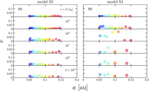
Snapshots of the system on the eccentricity – semimajor axis plane at t = 0, 105, 106, 107, 108, 2 × 10⁸tK. The left-hand panel (a) is the case M* = 1M⊙ and the right-hand panel (b) is that of M* = 0.2M⊙ as a typical mass of an M-type star. tK is one orbital period of the planet which has the closest orbit, 0.05 au at initial conditions. The size of each circle is proportional to the physical radius of the planet. The colour corresponds to each particle.
Next, we show the time evolution of the semimajor axis of the same run in Fig. 2. The number of planets gradually decreases and the orbital interval becomes wider. This giant impact process settles down in about 107–108tK. In panel (a), planets collide and merge mostly with their neighbors. This evolution is like a tournament chart. However, panel (b) is characterized by a large final eccentricity of the planet and frequent orbital crossings. As a result, the final planets have a large eccentricity and a wide spacing. In both models, no planets deviate from their initial distribution range.
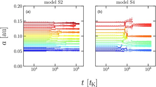
Time evolution of the semimajor axis (solid line) and distances of periapsis (dotted line) and apoapsis (dash–dotted line) for the same run as in Fig. 1 for model S2 (a) and model S4 (b).
The mass of the final planets are plotted against the semimajor axis for all 20 runs in models S2 and S4 together with the initial mass in Fig. 3. The planets are more linearly aligned in panel (a) than panel (b), which suggests that in model S2 the accretion proceeds locally keeping the initial global mass distribution. We theoretically estimate the possible mass distributions at each giant impact step. We assume that merging of adjacent planets in a tournament-like way. In a stage all neighbouring planets merge with each other. After merging, new planets are located at the position of the centre of mass of the merging planets. Planets in the nth stage are formed by n collisions and consist of 2n protoplanets. The growth pattern is like a tournament chart. In cases, there are an odd number of planets the seeding is incorporated as appropriate. The theoretical lines for planet masses formed by merging of two to eight protoplanets are shown in both panels. We find that in panel (a) the distribution of the final planets falls on this line nicely. This result does not apply to panel (b), since the giant impact takes place more globally as the stellar mass decreases.
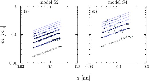
Mass of the final planets against the semimajor axis for all runs (filled circles) together with the initial conditions (open circles) for models S2 (a) and S4 (b). The blue lines show the theoretical predictions at each step of the tournament-like merger.
3.2 Stellar mass dependence
We now consider the planetary system parameters as a function of the stellar mass, and show the statistical results from 20 runs per model. Fig. 4 shows the number of planets 〈Nfin〉 and the maximum mass 〈mmax〉 of the final planetary system for models S1–S5. As the stellar mass increases, 〈Nfin〉 increases while 〈mmax〉 decreases. We can describe the dependence as 〈Nfin〉∝(M*/M⊙)0.379. This result shows that since the total disc mass is fixed, the maximum mass is inversely proportional to the number. We find that 〈mmax〉∝(M*/M⊙)−0.379. These power-law indices are consistent with the results of Matsumoto et al. (2020). Note that there is no ejection of planets from the system in all models.
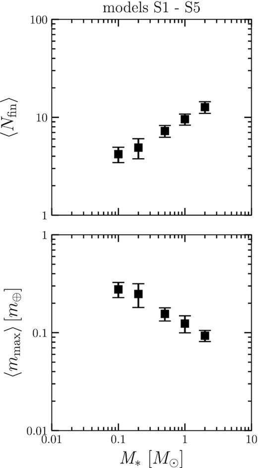
Stellar mass dependence of the final planets’ properties; average number of planets 〈Nfin〉 (top panel) and mass of the heaviest planet 〈mmax〉 (bottom panel) for models S1–S5. The error bar indicates the deviation.
Fig. 5 presents the stellar mass dependence of the system parameters. We find that 〈em〉, 〈im〉, 〈b〉, and 〈D〉 decrease with increasing M*. As shown in equation (2), the Hill radius is proportional to the −1/3 power of the stellar mass. Thus, a mass difference of a factor of 1/10 leads to a Hill radius difference of about twofold. Around low-mass stars, the gravitational interaction of planets is more effective due to the large Hill radius relative to the physical radius. As a result, the planet’s orbits are more disturbed, in other words, the eccentricity and inclination are larger. Therefore, the final state of a low-mass star planetary system has a large orbital separation on average. We also confirm that the orbital spacing normalized by the mutual Hill radius is within the range of about 19–23 for all stellar masses of models S1–S5.
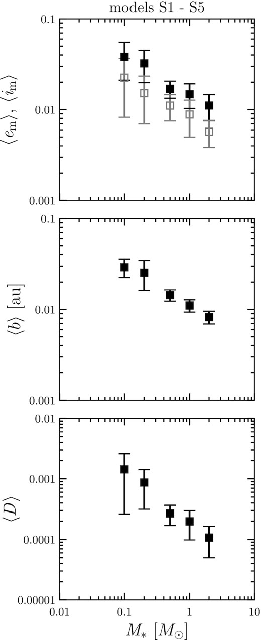
Stellar mass dependence of the mass-weighted eccentricity 〈em〉, inclination 〈im〉 (top panel), orbital separation 〈b〉 (middle panel), and AMD 〈D〉 (bottom panel) for models S1–S5.
3.2.1 Disc parameter dependence
We investigate the dependence of the planetary system architecture on the reference surface density Σ0 and initial orbital separation of protoplanets bini. We fix the stellar mass as |$0.2\, \mathrm{M}_\odot$|. Fig. 6 shows the number 〈Nfin〉 and the maximum mass 〈mmax〉 of the final planets against Σ0 (models S4, S6, and S7). We find that 〈mmax〉 and Σ0 have almost a linear relationship, |$\langle m_{\rm {max}} \rangle \propto \Sigma _0 ^{1.14}$|, which is consistent with the results of Kokubo et al. (2006) and Matsumoto et al. (2020). On the other hand, 〈Nfin〉 has a weak negative dependence on Σ0. Fig. 7 shows the relationship between 〈Nfin〉, 〈mmax〉, and bini (models S4, S8, and S9). The initial orbital separation does not change the results in the range of 5–10 Hill radius. In addition, Kokubo et al. (2006) showed that the initial orbital separation does not affect the properties of planets in the range of 6–12 Hill radius with |$M_* = 1\, \mathrm{M}_\odot$|. Our study confirms that this feature holds for low-mass stars. We also check the influence on the orbital structure. There are no effects for different Σ0 and bini on e and i.
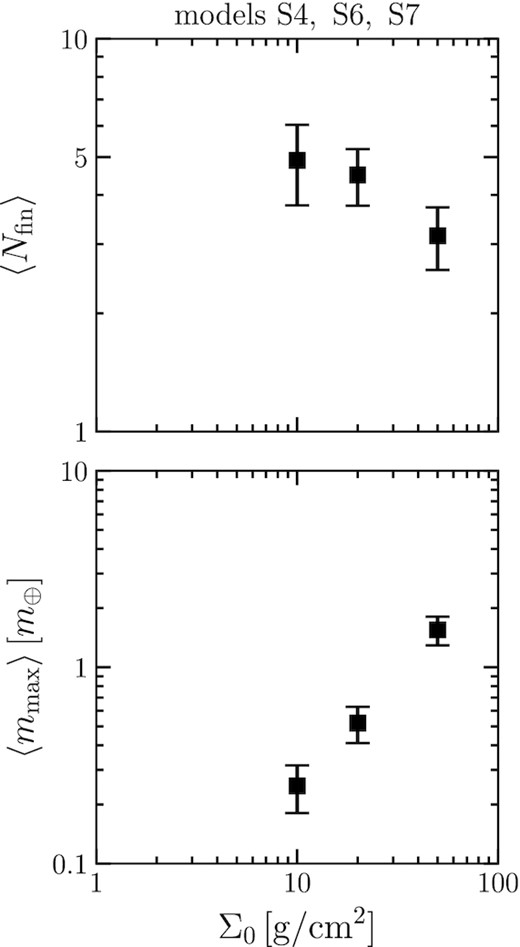
Relationship between the initial disc surface density and the mass of the planet (models S4, S6, and S7). It is clear that the higher the initial disc surface density, the larger the final planet. This dependence is almost linear.
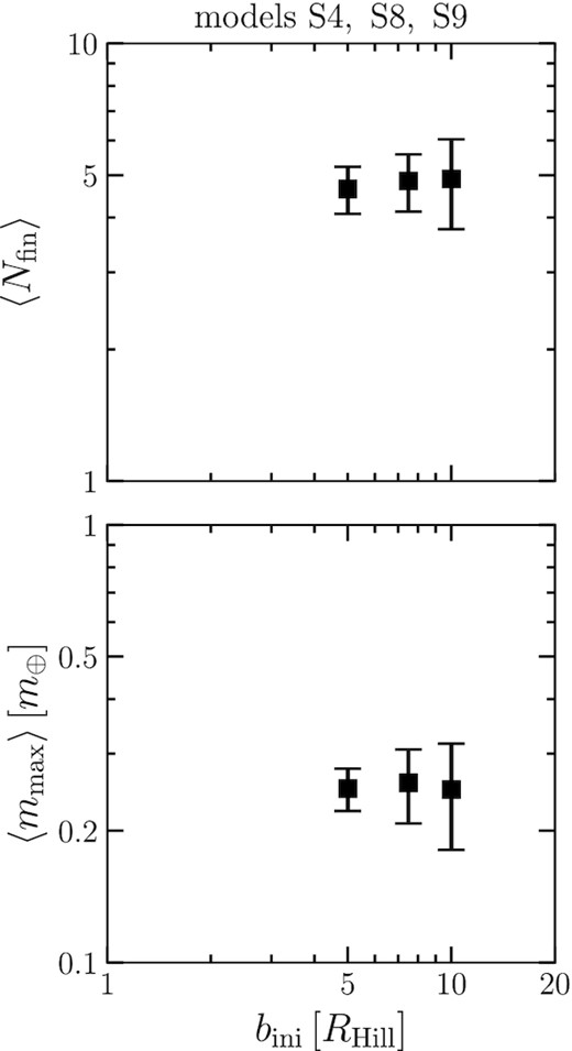
Relationship between the number of final planets 〈Nfin〉, the maximum mass of planets 〈mmax〉, and the initial orbital separation bini (models S4, S8, and S9).
3.2.2 MMEN model
Using the MMEN model, we investigate how the stellar mass and the disc model affect the structure of planetary systems with fixed orbital radius (models E1–E5). Fig. 8 shows the dependence of 〈Nfin〉, 〈mmax〉, and 〈D〉 on M*. We find that 〈Nfin〉 is almost constant. As shown in Section 3.2, the lower the stellar mass, the more the orbital structure is disturbed and the lower the number of planets. This effect is weakened by decreasing the surface density or disc mass in the MMEN model. On the other hand, 〈mmax〉 increase with M*, and have a relatively strong dependence, 〈mmax〉∝(M*/M⊙)1.41. As shown in Section 3.2.1, the planet mass increases with the disc surface density. In the MMEN model, this effect is more prominent than the others, reversing the dependence of 〈mmax〉 on M* in models S1–S5. The qualitative dependence of 〈D〉 on M* seems similar to that of the standard disc model. As M* increases, 〈D〉 becomes smaller. Compared to models S1–S5, 〈D〉 is generally larger. This is due to the larger planet masses.
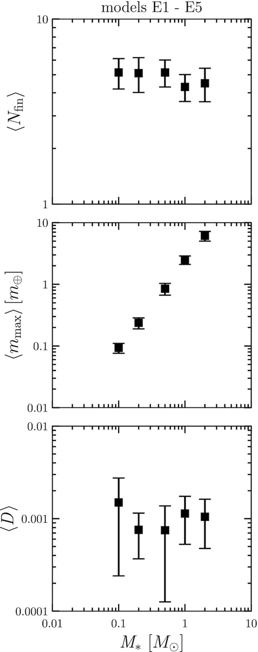
Stellar mass dependence of the number of final planets 〈Nfin〉 (top panel), maximum mass 〈mmax〉 (middle panel), and averaged AMD 〈D〉 (bottom panel) for MMEN disc models. The results for the number of planets in the top panel do not change much. In the middle panel, the planet mass is approximately proportional to the stellar mass.
3.3 Planets in the HZ
We focus on the planets in the HZ and examine their properties using the MMEN model (models EH1–EH4). Fig. 9 shows the dependence of the number and mass of planets on the stellar mass. The number of planets 〈Nfin〉 decreases as M* increases, while the maximum mass 〈mmax〉 increases with M*. This trend is consistent with the previous studies (e.g. Raymond et al. 2007; Ciesla et al. 2015). The prediction of the planetary masses in the HZ using our model and equation 2 of Raymond et al. (2007) results in |$M_{\rm {prediction}} \propto M_*^{1.7}$|, which shows a little bit shallower slope than our result |$\langle M_{\rm {max}} \rangle \propto M_*^{2.1}$|. In this prediction, the scaling factor of the stellar metallicity is originally included apart from the stellar mass. Our disc model incorporates the metallicity into the stellar mass, which may lead to a stronger dependence. As we have mentioned, the mass of the planets is directly affected by the disc surface density. Since the MMEN model is used, it is consistent that the planet mass and the stellar mass are positively correlated. In some simulation results of model EH1 there are no planets in the HZ. In the calculation of 〈Nfin〉, Nfin = 0 cases are included. For other values of orbital parameters, we exclude those runs.
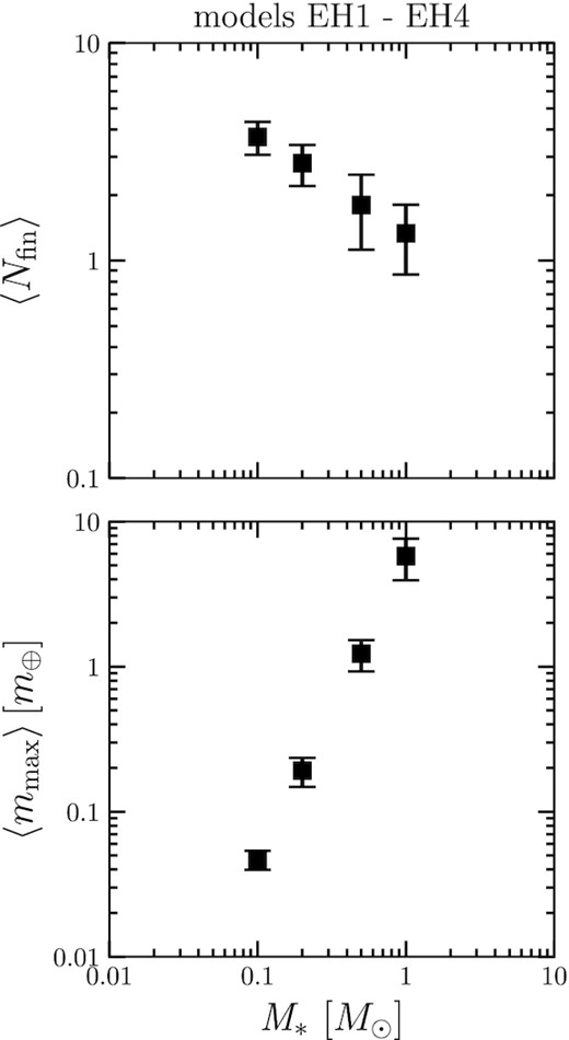
As Fig. 4, but for HZ planets with MMEN (models EH1–EH4).
Fig. 10 shows the orbital parameters of planetary systems. The orbital eccentricity 〈em〉 and inclination 〈im〉 increase with M* and the orbital separation 〈b〉 also increases with M*. When we consider planet formation in the HZ, we need to consider the balance between the effects of strengthening and weakening of gravitational scattering. As discussed in 3.2, with a fixed orbital radius, the Hill radius increases with decreasing stellar mass. In addition, for smaller stars, the HZ is closer and the Hill radius becomes smaller. The overall effect of these two factors is that gravitational scattering among protoplanets becomes weaker as the stellar mass decreases, because the distance from the star has a stronger effect. This can be understood in the following way: the smaller the stellar mass, the weaker the scattering, and thus 〈em〉, 〈im〉, and 〈D〉 become smaller.
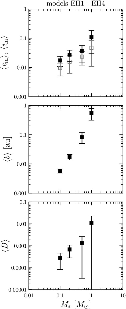
As Fig. 5, but for HZ planets with MMEN (models EH1–EH4).
If we know the orbital separation, then we can estimate the number of planets in the HZ. Based on the results in Fig. 10, if we divide the HZ width by the average orbital spacing, we can estimate the number of planets in the HZ to be 3.63, 2.61, 1.47, and 1.28 for M* = 0.1, 0.2, 0.5, and 1.0 M⊙, respectively. This estimate shows that the number of planets forming in the HZ decreases as the stellar mass increases. The number of planets in the HZ calculated from the orbital spacing agrees with the actual number of planets in the simulation results.
Finally, we summarize the results of all models in Table 2.
Final architecture of planetary systems.
| Model | 〈Nfin〉 | 〈mmax〉 | 〈em〉 | 〈im〉 | 〈b〉 | 〈D〉 |
|---|---|---|---|---|---|---|
| (m⊕) | (au) | (× 10−3) | ||||
| S1 | 12.7 | 0.0933 | 0.0111 | 0.00573 | 0.00823 | 0.107 |
| S2 | 9.55 | 0.124 | 0.0148 | 0.00884 | 0.0111 | 0.199 |
| S3 | 7.25 | 0.155 | 0.0169 | 0.0111 | 0.0144 | 0.268 |
| S4 | 4.90 | 0.248 | 0.0324 | 0.0152 | 0.0254 | 0.868 |
| S5 | 4.20 | 0.277 | 0.0381 | 0.0225 | 0.0292 | 1.43 |
| S6 | 4.50 | 0.518 | 0.0400 | 0.0190 | 0.0268 | 1.45 |
| S7 | 6.30 | 1.55 | 0.0620 | 0.0250 | 0.0142 | 3.25 |
| S8 | 4.85 | 0.257 | 0.0358 | 0.0218 | 0.0261 | 1.20 |
| S9 | 4.65 | 0.250 | 0.0373 | 0.0287 | 0.0277 | 1.57 |
| E1 | 4.50 | 6.11 | 0.0341 | 0.0190 | 0.0267 | 1.05 |
| E2 | 4.30 | 2.49 | 0.0377 | 0.0159 | 0.0267 | 1.14 |
| E3 | 5.15 | 0.850 | 0.0283 | 0.0156 | 0.0242 | 0.750 |
| E4 | 5.10 | 0.237 | 0.0306 | 0.0147 | 0.0238 | 0.758 |
| E5 | 5.15 | 0.0931 | 0.0400 | 0.0216 | 0.0256 | 1.50 |
| EH1 | 1.33 | 5.78 | 0.107 | 0.0468 | 0.549 | 11.1 |
| EH2 | 1.80 | 1.23 | 0.0362 | 0.0235 | 0.0835 | 1.33 |
| EH3 | 2.80 | 0.192 | 0.0274 | 0.0158 | 0.0173 | 0.680 |
| EH4 | 3.70 | 0.0467 | 0.0174 | 0.00957 | 0.00577 | 0.276 |
Note. Nfin is the number of final planets, mmax is the mass of the heaviest planet, em and im are the mass-weighted eccentricity and inclination, b is the orbital separation, and D is the angular momentum deficit. The ‘<>’ symbol indicates the average value of 20 runs.
4 SUMMARY AND DISCUSSION
We have performed N-body simulations of the giant impact stage of terrestrial planet formation changing the stellar mass from 0.1 to 2 M⊙ and examined the effect on the orbital structure of planetary systems. As the initial conditions, we adopted the isolation mass and distributed protoplanets in 0.05–0.15 au from the central star and the HZ. We followed the evolution for 200 million orbital periods of the innermost protoplanet. We investigated the effect of the initial disc parameters and also considered the minimum-mass extrasolar nebula (MMEN) model. Our findings are summarized as follows:
For a fixed orbital range and mass of the initial protoplanet distribution, the number of planets 〈Nfin〉 increases with the stellar mass M*, while the maximum mass of the planets 〈mmax〉 decreases. The eccentricity 〈em〉, inclination 〈im〉, and orbital separation 〈b〉 of planet orbits decrease with increasing M*. This is because gravitational interactions among protoplanets become relatively stronger as M* decreases.
As the total mass of protoplanets increases, 〈Nfin〉 decreases, while 〈mmax〉 increases.
The initial orbital separation of protoplanet systems in the range of 5–10 Hill radius does not affect the final orbital structures.
In the MMEN model, 〈mmax〉 increases with M*.
In the HZ of the MMEN model, 〈Nfin〉 decreases with M*, while 〈mmax〉 increases. Other orbital parameters 〈em〉, 〈im〉, and 〈b〉 increase with M*.
In this study, the surface density slope α is fixed. The dependence of α has been discussed in many papers in the case of one solar mass (e.g. Raymond et al. 2005; Kokubo et al. 2006; Ronco & de Elía 2014; Izidoro et al. 2015). We confirmed that the stellar mass dependence remains the same for different α. Details will be discussed in the next paper.
Our results show that orbital separations of planets are 17–26 Hill radii for all models. This is consistent with the Kepler planets that are about 20 Hill radii apart (e.g. Weiss et al. 2018). We can also reproduce planets in the smaller mass side of the CKS samples (Johnson et al. 2017; Petigura et al. 2017) used in the MMEN model. However, since there are still few planets around low-mass stars, our results below one solar mass are rather predictive. Our concern is that planet masses are inferred from radii in the construction of the MMEN models. The mass–radius relation used in Dai et al. (2020) does not yet reflect the latest exoplanet observations. In addition, when only planets with known masses by the radial velocity and transit timing variation methods are used, the disc surface density is found to be about twice as large. The absolute values of disc surface densities are still quite uncertain. Considering this shortage of data and the uncertainty of the mass–radius relation, it is necessary to reconsider the MMEN model, at least for planets around low-mass stars.
It is meaningful to investigate whether the characteristics of planetary systems observed around 1 M⊙ stars are also observed around low-mass stars. Here, we focus on the radius ratio of neighbouring planet pairs. We convert planet mass to radius using Eq. (8). Though we have 20 planetary systems per model, we do not consider which system they belong to but treat all of them equally as a planet pair. Fig. 11 shows the correlation between the radii of the inner and outer planets for model S2. Neighbouring planets tend to have the same size. In addition, we plot the number of planet pairs against the radius ratio of the outer to inner planets in Fig. 12. We find that the radius ratio distribution has a peak around 1.

Radius of a planet Rin versus that of the next planet Rout for model S2. The blue line indicates Rin = Rout.
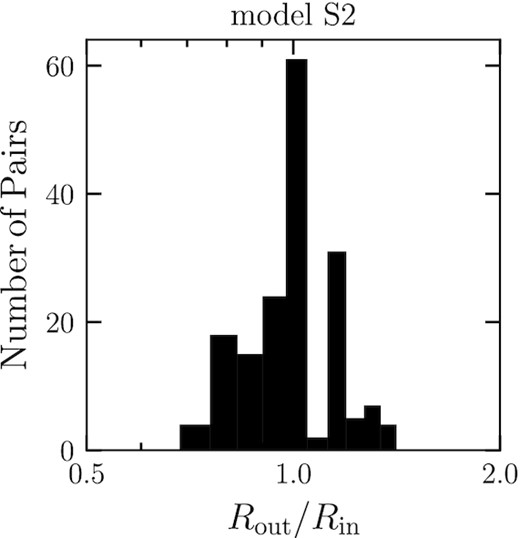
Histogram of the radius ratio of adjacent planet pairs for model S2.
We show the radius ratio of neighbouring pairs against the stellar mass in Fig. 13 (models S1–S5) together with the theoretical prediction. The theoretical prediction is based on the tournament-like growth discussed in Section 3.1. We also used the number of planets and orbital separation obtained in the simulations. We find that the radius ratio of neighbouring planets does not depend on the stellar mass. These analyses conclude that the neighbouring planets have similar radii in planetary systems around ∼0.1 au if the initial protoplanet mass does not strongly depend on the orbital radius, which is consistent with the peas-in-a-pod pattern seen in the Kepler multiple-planet system (e.g. Weiss et al. 2018).

Mean radius ratio of adjacent planet pairs (black squares) plotted against the stellar mass for models S1–S5 with the theoretical predictions (blue circles). The error bars represent the deviation.
In this study, we mainly focused on the dependence of the orbital structure of planetary systems on the stellar mass. In reality, the orbital structure may depend on disc and protoplanet parameters that are not considered here. A comparison using dimensionless orbital parameters such as those normalized by the Hill radius is helpful for physical understanding of the structure dependence. By performing a systematic parameter survey, we will generalize the orbital parameter dependence and discuss a new basic scaling law of the structure that incorporates not only gravitational interaction but also collisions among planets in the next paper.
ACKNOWLEDGEMENTS
Numerical computations were carried out on PC cluster at Center for Computational Astrophysics, National Astronomical Observatory of Japan. E.Kokubo is supported by JSPS KAKENHI grant no. 18H05438.
DATA AVAILABILITY
All data underlying this research are included in the article.
