


ABSTRACT
Sophisticated spectral energy distribution (SED) models describe dust attenuation and emission using geometry parameters. This treatment is natural since dust effects are driven by the underlying star–dust geometry in galaxies. An example is the starduster SED model, which divides a galaxy into a stellar disc, a stellar bulge, and a dust disc. This work utilizes the starduster SED model to study the efficacy of inferring geometry parameters using spatially integrated SED fitting. Our method fits the SED model to mock photometry produced by combining a semi-analytic model with the same SED model. Our fitting results imply that the disc radius can be constrained, while the inclination angle, dust disc to stellar disc radius ratio, bulge radius, and intrinsic bulge to total luminosity ratio are unconstrained, even though 21 filters from ultraviolet to far-infrared are used. We also study the impact of signal-to-noise (S/N) ratio, finding that the increase of S/N (up to 80) brings limited improvements to the results. We provide a detailed discussion to explain these findings, and point out the implications for models with more general geometry.
1 INTRODUCTION
Spectral energy distribution (SED) fitting is a fundamental method to infer galaxy properties. These techniques have been applied to measure stellar masses, star formation rates, metallicities, dust masses, and dust attenuation curves (e.g. Leja et al. 2017; Driver et al. 2018; Bellstedt et al. 2020; Qin et al. 2022). What parameters can be inferred using SED fitting depends on how the SED is parametrized. A state-of-the-art SED code (e.g. Boquien et al. 2019; Robotham et al. 2020; Johnson et al. 2021) describes an SED using parameters of star formation history (SFH), dust attenuation, dust emission, and active galactic nucleus.
An improvement of SED models could be the implementation of a more physical dust model. Currently, the dust attenuation curve in most SED models is described by a phenomenological model, e.g. a power law with additional parameters specifying the shape of the |$2175 \, {\mathring{\rm A}}$| bump. This method can be improved by taking into account more detailed star–dust geometry. For instance, the geometry can be parametrized using analytic density profiles. Given the geometry model, one can predict both dust attenuation and emission self-consistently using radiative transfer simulations (e.g. Camps & Baes 2020; Narayanan et al. 2021). Following this approach, the SED is described by geometry parameters, and therefore one can infer these parameters by fitting the SED to observations. However, the application of SED models based on radiative transfer simulations (e.g. De Geyter et al. 2013; Fioc & Rocca-Volmerange 2019) is not straightforward due to their high computational cost. Recently, this issue was partially overcome by Qiu & Kang (2022), who applied deep learning neural networks to accelerate the speed of a radiative transfer simulation. The SED model proposed by Qiu & Kang (2022) describes dust attenuation and emission using geometry parameters. The model is named as starduster, and is publicly available on Github.1
With the dust model in SED codes becoming more sophisticated, a natural question is whether the geometry parameters underlying the model can still be constrained using SED fitting. This work aims to address this question by fitting the starduster SED model to mock photometric data produced by coupling the same SED model with a semi-analytic model. This approach provides insights into the dependence of the SED on the geometry parameters. We then extend our discussion into more general geometry.
This paper is organized as follows. We introduce the starduster SED model, the construction of the mock data, and the method of SED fitting in Section 2. The fitting results are presented in Section 3, followed by a detailed discussion in Section 4. Finally, this work is summarized in Section 5.
2 METHODOLOGY
2.1 The SED model
2.2 Mock photometry
To construct a mock photometric catalogue, we combine the starduster SED model with a semi-analytic galaxy formation model. This work adopts the semi-analytic model presented by Luo et al. (2016), which is a modified version of the L-Galaxies model (Kauffmann 1996; De Lucia & Blaizot 2007; Guo et al. 2011, 2013; Fu et al. 2013). The model builds on the halo merger trees constructed from the Millennium Simulation (Springel et al. 2005). Physics implemented in the model includes gas cooling, star formation, supernova feedback, metal production, bulge formation, and active galactic nuclei feedback. Luo et al. (2016) verified that the model can reproduce the stellar, H1 and H2 mass functions at z ∼ 0. The reader is referred to Guo et al. (2011), Fu et al. (2013), and Luo et al. (2016) for a detailed description of the model.
The required galaxy parameters by the starduster SED model are listed in Table 1. In our semi-analytic model, the disc radius is proportional to the spin parameter and virial radius of the host halo. Fu et al. (2013) showed that this treatment leads to a median stellar surface density that is broadly consistent with the observations by Leroy et al. (2008). The bulge radius is predicted by the bulge formation model introduced in Guo et al. (2011), who demonstrated that their results agree with the observed half-mass radius of early-type galaxies by Shen et al. (2003). The intrinsic bolometric luminosity, bulge to total luminosity ratio, and luminosity fractions are converted using the predicted disc mass, bulge mass, and SFH of the stellar disc and bulge. Additionally, we draw the inclination angle uniformly from a unit sphere.
Full parameters of the starduster SED generative model.
| Symbol | Description | Range |
|---|---|---|
| θ | Inclination angle | 0–90 deg |
| rdisc | Stellar disc radius | 10−2.5 to 102.5 kpc |
| rbulge | Stellar bulge radius | 10−0.5 to 101.5 kpc |
| qdust | Dust disc radius to stellar disc radius (DTS) ratio | 10−0.7 to 100.7 |
| Σdust | Dust surface densitya | |$10^{3.0} - 10^{7.5} \, \text{M}_\odot \, \text{kpc}^{-2}$| |
| lnorm | Intrinsic bolometric luminosity | |$10^6 - 10^{14} \, \text{L}_\odot$| |
| αB/T | Intrinsic bulge to total luminosity ratio | 0–1 |
| |$c^{\rm disc}_{i,k}$| | Luminosity fraction of the stellar disc in the i-th metallicity bin and the k-th stellar age binsb | 0–1 |
| |$c^{\rm bulge}_{i,k}$| | Luminosity fraction of the stellar bulge in the i-th metallicity bin and the k-th stellar age binb | 0–1 |
Notes.aDust surface density is defined by |$\Sigma _\text{dust} = m_\text{dust} / (2\pi r^2_\text{dust})$|.
b There are six metallicity and six stellar age bins in the starduster model.
We compute the fluxes in 21 filters from ultraviolet (UV) to far-infrared (FIR) for each galaxy. The adopted filters are shown in Fig. 1. In addition to the commonly used filters, we also include a top-hat filter at |$40 \, \rm{\mu m}$|. This is motivated by our previous study (Qiu & Kang 2022), who found that the extra data could improve the measurement of bulge size. Moreover, we perturb the fluxes in all bands. We assume the same signal-to-noise (S/N) ratio in all bands, and adopt S/N values of 5, 10, 20, 40, and 80.
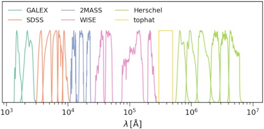
Adopted filters for the mock photometry.
We select model galaxies as follows. First, as listed in Table 1, each input parameter of the starduster SED has an allowed range, and we only include galaxies whose properties are within these ranges. In our model, a majority of low stellar mass galaxies have zero dust mass, which are excluded in this step. Most of these galaxies are satellites. The cold gas in these galaxies is removed by ram pressure stripping. Secondly, we only study galaxies at z = 0. The model produces millions of galaxies at z = 0, and it is unnecessary to include all of them. Instead, we randomly select 5000 galaxies for the catalogue. Fig. 2 illustrates the distribution of some relevant properties in the mock catalogue.

Upper panels: Distribution of stellar disc radius, bulge radius, DTS ratio, and dust surface density in the mock galaxy catalogue. Lower panels: Distribution of dust mass, stellar mass, V-band attenuation, and total IR luminosity in the mock galaxy catalogue. All y-axes are in a linear scale. The construction of the catalogue is described in Section 2.2.
2.3 SED fitting
The application of the starduster model to SED-fitting requires a parametrization of the SFH and metallicity history (MH). As listed in Table 1, the starduster model has 79 input parameters, which might be unsuitable for SED fitting. Our proposed model for SED fitting has 13 or 17 free parameters, which are described as follows. A summary of these parameters is given in Table 2.
Simplified parameters of the starduster SED fitting model.
| Symbol | Description | Modela | Scale | Unit | Range |
|---|---|---|---|---|---|
| θ | Inclination angle | Linear | deg | 0–90 | |
| rdisc | Stellar disc radius | Log | kpc | −2.0 to 2.5 | |
| rbulge | Stellar bulge radius | Log | kpc | −0.5 to 1.5 | |
| qdust | Dust disc radius to stellar disc radius (DTS) ratio | Log | – | −0.7 to 0.7 | |
| Σdust | Dust surface densityb | Log | |$\text{M}_\odot \, \text{kpc}^{-2}$| | 3.0–7.5 | |
| lnorm | Intrinsic bolometric luminosity | Log | L⊙ | 6–14 | |
| αB/T | Intrinsic bulge to total luminosity ratio | Linear | – | 0–1 | |
| |$a_1^\text{disc}$| | Transformed luminosity fraction for 1–4 Myr | Discrete SFH | Linear | – | 0–1 |
| |$a_2^\text{disc}$| | Transformed luminosity fraction for 4–24 Myr | Discrete SFH | Linear | – | 0–1 |
| |$a_3^\text{disc}$| | Transformed luminosity fraction for 24–118 Myr | Discrete SFH | Linear | – | 0–1 |
| |$a_4^\text{disc}$| | Transformed luminosity fraction for 118–580 Myr | Discrete SFH | Linear | – | 0–1 |
| |$a_5^\text{disc}$| | Transformed luminosity fraction for 580 Myr–2 Gyr | Discrete SFH | Linear | – | 0–1 |
| |$a_6^\text{disc}$| | Transformed luminosity fraction for 2–14 Gyr | Discrete SFH | Linear | – | 0–1 |
| τdisc | Star formation time-scale | Exponentially declining SFH | Log | yr | 9.1–12.1 |
| |$t^\text{disc}_0$| | Star formation start time | Exponentially declining SFH | Log | yr | 6.0–10.1 |
| |$Z_\text{final}^\text{disc}$| | Maximum metallicity | Log | Z⊙ | −2.62 to 0.12 | |
| ξdisc | Metallicity ratio | Log | – | −3 to 0 | |
| cbulge | Luminosity fraction for 580 Myr–2 Gyr | Linear | – | 0–1 | |
| Zbulge | Bulge metallicity | Log | – | −2.62 to 0.12 |
Notes.aWe adopt two different SFH models for the stellar disc as described in Section 2.3.
bDust surface density is defined by |$\Sigma _\text{dust} = m_\text{dust} / (2\pi r^2_\text{dust})$|.
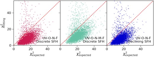
Relation between the best fitting and expected χ2. The expected χ2 is defined by the unperturbed and perturbed fluxes, and is calculated by replacing |$f^\text{pred}_i$| in equation (9) with the unperturbed fluxes. These panels compare the results that include more filters or adopt a simpler SFH model. The two filter sets, i.e. UV-O-N-F and UV-O-N-M-F are described in Section 2.2. The discrete and declining SFH models are introduced in Section 2.3.
For the stellar bulge, we assume that this component only consists of old stellar populations. Specifically, we restrict the presence of non-zero luminosity fractions to the oldest two age bins. Due to the normalization, the bulge SFH is characterized by only one parameter. Additionally, the MH of the stellar bulge is assumed to be constant, which can be described by one parameter.
We consider the following variations in our SED fitting analysis:
We fit our SED model to two filter sets, labelled as UV-O-N-M-F and UV-O-N-F. The former includes all 21 filters demonstrated in Fig. 1. This filter set covers almost all wavelengths from UV to FIR, which is used to test whether the geometry parameters can be constrained in the ideal case. For the UV-O-N-F set, we exclude the fluxes from the WISE and top-hat filters. In practice, MIR data are sensitive to dust grain composition, which is fixed in the starduster SED model. For both fitting processes, we assume an S/N of 20 and adopt the discrete SFH.
We carry out a fitting process that uses the exponentially declining SFH for the stellar disc. As will be shown in Section 3, the model based on the discrete SFH is overfitted. We test whether the overfitting can be reduced by using a simpler model. For this run, we choose the UV-O-N-F filter set and adopt an S/N of 20.
The impact of S/N is also examined. Our SED model is fit to the mock data with S/N values of 5, 10, 20, 40, and 80. In each case, we use the UV-O-N-F filter set and assume the discrete SFH model.
3 RESULTS
3.1 Goodness of fit
We start by examining the goodness of fit. Fig. 3 compares the best-fitting and expected χ2 values. The expected values are calculated by replacing |$f^\text{pred}_i$| in equation (9) with the unperturbed fluxes. As shown in Fig. 3, the best-fitting χ2 values are generally lower than the expected ones. While this confirms the convergence of our fitting algorithm, it also indicates overfitting. As illustrated in the middle and left-hand panels of Fig. 3, including more filters or using a simpler model cannot resolve the issue. An implication is that the parameter space of our SED has strong degeneracies. Despite the problem, as will be shown below, we can still recover some of the galaxy properties.
3.2 Recovery of SFHs and MHs
The upper panels of Fig. 4 compare the inferred SFHs with the input mock data. When using the discrete SFH model, we can recover the median mass fractions of the stellar disc in all age bins and those of the stellar bulge in the oldest age bin. However, for the total SFH, consistent results are only found in the 580 Myr <t < 14 Gyr age bins. An implication is that the bulge to total luminosity ratio is unconstrained. When using the exponentially declining SFH, we fail to recover the disc SFH. However, for the total SFH, except the 24 Myr <t < 580 Myr age bins, the inferred median mass fractions are consistent with the input mock data.
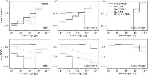
Recovery of SFHs and MHs. The upper and lower panels show the median mass fraction and metallicity as a function of stellar age respectively. Each panel compares the results that include more filters or adopt a simpler SFH model. The two filter sets, i.e. UV-O-N-F and UV-O-N-M-F are described in Section 2.2. The red and green line results are based on the discrete SFH, while the blue line results are based on the exponentially declining SFH. Both SFH models are described in Section 2.3.
The bottom panels of Fig. 4 demonstrate the recovery of MHs. In all cases, we cannot obtain consistent results. We note that our proposed MH model in Section 2.3 depends on the SFH. Consequently, if the SFH cannot be well recovered, we will fail to obtain consistent MH. Despite this discrepancy, as shown in Fig. 5, we call still constrain the mass-weighted metallicity.
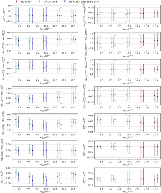
Distribution of the error between the ground truth and best-fitting parameters as a function of stellar mass. Each panel compares the results that include more filters or adopt a simpler SFH model. We introduce the two filter sets, i.e. UV-O-N-F and UV-O-N-M-F in Section 2.2. The discrete and exponentially declining SFH models are described in Section 2.3. The properties in the left-hand panels are the direct input parameters of the SED model as listed in Table 2. In the right-hand panels, from top to bottom, the properties are mass-weighted metallicity, star formation rate, stellar mass, dust mass, total infrared luminosity, UV band dust attenuation, and V-band dust attenuation. The star formation rate time-scale is 100 Myr.
3.3 Recovery of galaxy parameters
In Fig. 5, we show the error of some recovered galaxy properties as a function of stellar mass. The error is defined by the difference between the truth and best-fitting values for each galaxy. We first focus on the results based on the UV-O-N-F filter set and the discrete SFH, corresponding to the red circles with error bars. The errors in the derived disc radius range from −0.2 to 0.25 dex in the low-mass end and from −0.25 to 0.5 dex in the high-mass end. This implies that the disc radius can be constrained, given that the input disc radius varies over 2 orders of magnitude as shown in Fig. 2. In contrast, the errors in the inferred DTS ratio range from −0.3 to 0.4 dex, which is greater than the intrinsic scatter, i.e. 0.2 dex. Additionally, this property is also systematically overestimated in the high stellar mass end. Hence, the DTS ratio is unconstrained. Similarly, the errors in the inferred inclination angle are comparable with its allowed range, implying that this quantity is also unconstrained. Moreover, the best-fitting bulge radii and intrinsic bulge to total luminosity ratios show large systematic offsets. Therefore, we fail to infer these properties using SED fitting.
When including more data in MIR to FIR wavelengths, as illustrated in Fig. 5, the fitting results are only slightly improved. Using the same SED model, Qiu & Kang (2022) found that the measurement of the bulge radius can be improved when including data at |$\sim 40 \, \rm{\mu m}$| in the SED fitting of two observed galaxies. However, our results in Fig. 5 indicate that the |$40 \, \rm{\mu m}$| flux in general is insufficient to recover the bulge radius. In addition, the other unconstrained parameters, i.e. the inclination angle, DTS ratio, bulge radius and intrinsic bulge to total luminosity ratio remain unconstrained when including more data.
Fig. 5 also illustrates the fitting results based on the exponentially declining SFH. In general, these results are similar to those based on the discrete SFH. A difference is that the inferred stellar mass and star formation rate show more bias. The reason is that the exponentially declining SFH model is not flexible enough to fit the mock data, which was discussed in great detail in previous studies (Carnall et al. 2019; Leja et al. 2019; Lower et al. 2020).
3.4 Trends with S/N
We demonstrate the impact of S/N on the SED fitting results in Figs 6, 7, and 8. These results are based on the UV-O-N-F filter set and the discrete SFH. In Fig. 6, we find that increasing the S/N cannot resolve the overfitting problem. Particularly, with the increase of the S/N, many results show a substantially large χ2 value, meaning that the SED model cannot fit the mock data. We compare the inferred SFHs and MHs at different S/N values in Fig. 7. In general, higher S/N values lead to more consistent results. However, the improvement becomes less significant when the S/N is increased from 20 to 80. A similar trend is found in the recovery of galaxy parameters as illustrated in Fig. 8. In particular, varying the S/N has no impact on the inferred inclination angle, bulge radius and intrinsic bulge to total luminosity ratio, which are all unconstrained parameters. All these findings imply that high S/N data cannot break the degeneracies in the SED model. In other words, the improvements from high S/N data are limited. A similar conclusion was obtained by Leja et al. (2019), who found that the chosen prior of the SFH can have a larger impact on the fitting results than the photometric noise.
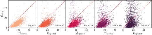
Relation between the best fitting and expected χ2 as a function of S/N. The expected χ2 is defined by the unperturbed and perturbed fluxes, and is calculated by replacing |$f^\text{pred}_i$| in equation (9) with the unperturbed fluxes. These results are based on the UV-O-N-F filter set (see Section 2.2) and the discrete SFH model (see Section 2.3).

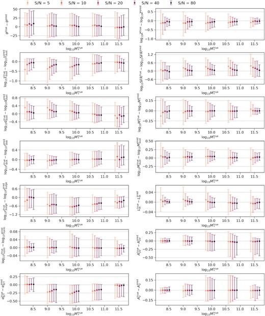
Distribution of the error between the ground truth and best-fitting parameters as a function of stellar mass. Each panel compares the results for different S/N values. These results are based on the UV-O-N-F filter set (see Section 2.2) and the discrete SFH model (see Section 2.3). The properties in the left-hand panels are the direct input parameters of the SED model as listed in Table 2. In the right-hand panels, from top to bottom, the properties are mass-weighted metallicity, star formation rate, stellar mass, dust mass, total infrared luminosity, UV band dust attenuation, and V-band dust attenuation. The star formation rate time-scale is 100 Myr.
4 DISCUSSION
From our fitting results presented in the previous section, we conclude that the disc radius can be constrained, while the DTS ratio, bulge radius, intrinsic bulge to total luminosity ratio, and inclination angle are unconstrained or poorly constrained. To interpret the results, we need to understand how the SED depends on these parameters. In Fig. 9, we increase the input SED parameters by a factor of 2, and illustrate the resulting variance in some selected bands. The inclination angle is not in a logarithmic scale and is increased by 15 deg instead. The shape of the FIR spectrum can be characterized more intuitively using the total infrared luminosity and the peak wavelength of the FIR emission. Hence, we also show the variance of these two quantities in Fig. 9.
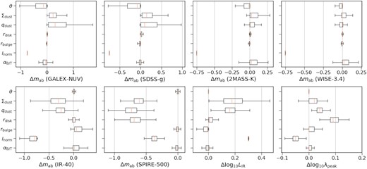
Dependence of the SED on the input parameters. Each panel shows the variance of the AB magnitude in a filter when the input SED parameters are increased by a factor of 2, except the inclination angle, which is increased by 15 deg. In addition, the third and fourth panels in the bottom show the variance of the total infrared luminosity and the peak of the FIR emission, respectively. These results are based on the mock galaxy catalogue described in Section 2.2. The definition of the varied parameters can be found in Table 2.
4.1 Disc radius
Fig. 9 illustrates that increasing the disc radius (at fixed DTS ratio) has no impact on the UV to optical SED but leads to the largest shift in the peak of the FIR emission. Besides the disc radius, the peak of the FIR emission is also sensitive to the intrinsic bolometric luminosity and the DTS ratio. The former gives the overall normalization of the SED, and can be constrained by the UV to NIR fluxes. The latter has a small allowed range, and therefore cannot substantially change the absolute value of the peak wavelength. In other words, the degeneracies between the disc radius and these parameters are insignificant. Hence, the disc radius can be constrained by the peak of the FIR emission.
The dependence of the SED on the disc radius found in this work was explained in the radiative transfer study by Misselt et al. (2001). They suggested that varying the physical size of a dusty system with all the other quantities fixed does not change the total optical depth, and hence has no effect on the UV to optical spectrum. Misselt et al. (2001) also pointed out that the dust temperature depends on the ratio of the absorbed energy to the dust mass. In our model, increasing the disc radius at fixed dust surface density and DTS ratio results in higher dust mass and therefore lower dust temperature, which shifts the peak of the FIR emission to longer wavelengths.
4.2 Dust surface density and DTS ratio
Fig. 9 shows that varying the dust surface density and the DTS ratio influences the UV to FIR fluxes in a similar way. However, only the dust surface density is constrained. A potential reason is that the allowed range of dust surface density is much larger than the DTS ratio. As listed in Table 2, the dust surface density can span over 4 orders of magnitude, while log10qdust is only allowed to vary from −0.7 to 0.7. Hence, the dust surface density is the primary factor that determines the amount of dust attenuation, while the DTS ratio is a secondary term.
4.3 Bulge radius and intrinsic bulge to total luminosity ratio
Our results suggest that the bulge radius and the intrinsic bulge to total luminosity ratio cannot be constrained. To explain the reason, we need to understand how the SED depends on these quantities. If we assume that the stellar disc and bulge have the same stellar population, varying rbulge and αB/T will similarly impact the SED. This point is demonstrated in Fig. 10. Decreasing the bulge radius or the intrinsic bulge to total luminosity ratio increases the fraction of light that is obscured by the dust disc. This effect reddens the UV to optical colour for highly inclined galaxies but is negligible for face-on galaxies. In MIR to FIR wavelengths, the decrease of the bulge radius or the intrinsic bulge to total luminosity ratio increases the absorbed energy and therefore the dust temperature. This slightly shifts the peak of the FIR emission to shorter wavelengths and increases the MIR to FIR fluxes. A similar effect of the intrinsic bulge to total luminosity ratio on the FIR spectrum was found by Popescu et al. (2011). In addition, when the stellar disc and bulge have different stellar populations, varying αB/T can influence the NIR flux as shown in Fig. 9, which, however, can be mimicked by the SFH parameters.
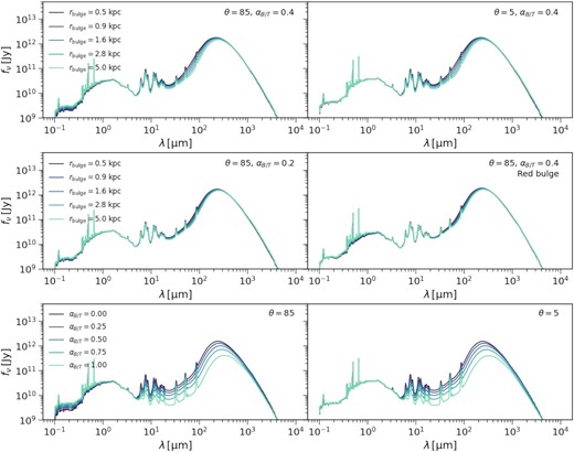
Upper and middle panels: dependence of the SED on the bulge radius at different inclination angles, intrinsic bulge to total luminosity ratios, and stellar populations. Lower panels: dependence of the SED on the intrinsic bulge to total luminosity ratio. The base SED and adopts |$\Sigma _\text{dust} = 10^5 \, \text{M}_\odot / \text{kpc}^2$|, |$r_\text{disc} = 5 \, \text{kpc}$|, qdust = 1, |$r_\text{buge} = 1 \, \text{kpc}$|, and |$l_\text{norm} = 10^9 \, \text{L}_\odot$|. The SFH is assumed to be constant from 1 Myr to 14 Gyr, with Z = 0.1Z⊙. For the red bulge variant, the stellar population from 580 Myr to 14 Gyr is in the bulge, with the overall SFH kept constant.
We further point out two factors that weaken the dependence of the SED on the bulge radius. They are illustrated in the middle panels of Fig. 10. First, the effect of varying the bulge radius is only significant for large αB/T. Secondly, the dust effect of the bulge will be less pronounced if the bulge is dominated by old stellar populations.
In short, varying the bulge radius and intrinsic bulge to total luminosity ratio only has moderate effects on the UV to optical and MIR to FIR fluxes, and there is a strong degeneracy between both parameters. Therefore, these parameters cannot be constrained using SED fitting.
4.4 Inclination angle
The inclination angle is also an unconstrained parameter. A potential reason is that the inclination angle is irrelevant to the dust emission spectrum but degenerates with all the other parameters in the UV to optical regime.
Since the inclination angle can be measured using galaxy images, it is instructive to check the fitting results with this parameter fixed. Such results are presented in Figs 11, 12, and 13. A major improvement is that the 1σ offsets of the UV and V-band attenuation are reduced by ∼0.1 mag, while the estimations of the other galaxy parameters and the SFHs are unaffected. The impact of the inclination on measuring dust attenuation was also highlighted by Doore et al. (2022), who carried out an SED-fitting analysis on 151 disc-dominated galaxies using an inclination-dependent model.
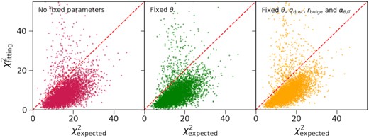
Relation between the best fitting and expected χ2. The expected χ2 is defined by the unperturbed and perturbed fluxes, and is calculated by replacing |$f^\text{pred}_i$| in equation (9) with the unperturbed fluxes. These panels compare the results when certain parameters are fixed in the fitting. These results are based on the UV-O-N-F filter set (see Section 2.2) and the discrete SFH model (see Section 2.3).
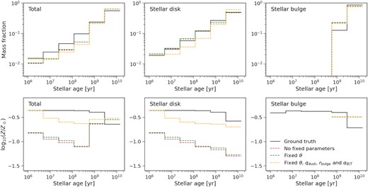
Impacts of fixing certain parameters in the fitting on the inferred SFHs and MHs. The upper and lower panels show the median mass fraction and metallicity as a function of stellar age respectively. Each panel compares the results when certain parameters are fixed in the fitting. These results are based on the UV-O-N-F filter set (see Section 2.2) and the discrete SFH model (see Section 2.3). For the mass fractions, the results with no parameters fixed overlap those with the inclination angle fixed.
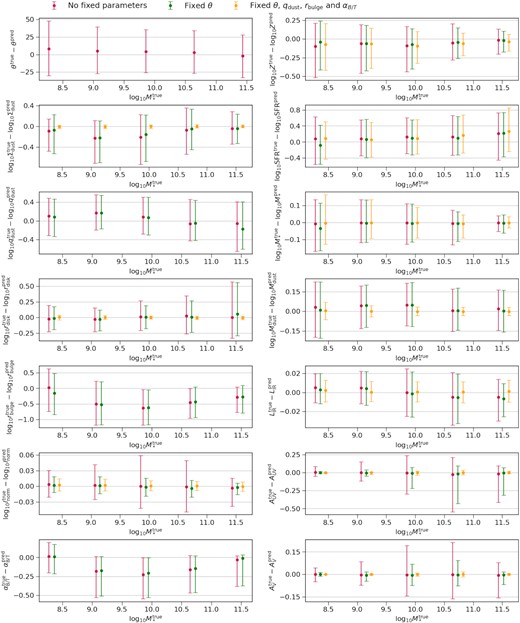
Impacts of fixing certain parameters in the fitting on the inferred galaxy properties. Each panel shows the error between the ground truth and best-fitting parameters as a function of stellar mass. No data points will be plotted if the property is fixed. These results are based on the UV-O-N-F filter set (see Section 2.2) and the discrete SFH model (see Section 2.3). The properties in the left-hand panels are the direct input parameters of the SED model as listed in Table 2. In the right-hand panels, from top to bottom, the properties are mass-weighted metallicity, star formation rate, stellar mass, dust mass, total infrared luminosity, UV band dust attenuation, and V-band dust attenuation. The star formation rate time-scale is 100 Myr.
4.5 More general geometry
Our discussion above can be generalized to different geometry models. Galaxy geometry is more complex and diverse in reality, which in general could not be described by the density profiles introduced in Section 2.1. However, the spatial distribution of stars and dust grains are correlated, since dust grains are produced by supernova and stellar winds. Accordingly, the star–dust geometry could be described by a common characteristic scale, with higher order terms quantifying the differences between the stellar and dust discs. Our analysis in Section 4.1 implies that the common characteristic scale should have limited effects on the UV to optical spectrum but dramatically influence the peak of the FIR emission. Therefore, for a SED model with more complex geometry, we should be able to constrain the characteristic scale using FIR data. For the higher order terms, an analogue is the DTS ratio in our SED model. As illustrated in Fig. 9, this parameter can impact all UV to FIR fluxes. However, as discussed in Section 4.2, the DTS ratio cannot be constrained due to its small allowed range. For the same reason, we expect that spatially integrated SED fitting cannot constrain the differences between the distribution of stars and dust in general. In addition, our discussion in Section 4.3 suggests that we are also unable to constrain bulge related properties.
4.6 Improvement
Our analysis implies that not all geometry parameters can be constrained using the spatially integrated SED, and a potential improvement is to combine SED fitting with image analysis tools. Such an idea was presented by Popescu et al. (2011) and Robotham, Bellstedt & Driver (2022). A typical profile fitting tool (e.g. Peng et al. 2010) can estimate inclination angle, disc size, bulge size, and bulge to total luminosity ratio. One could also extract dust disc size from FIR images. These parameters are also inputs of the starduster SED model. Hence, we can fit the SED and the light profile jointly.
A question is what can be improved when the unconstrained parameters in our SED model are determined using the extra information from galaxy images. To demonstrate, we perform an additional SED fitting process with all the unconstrained parameters fixed. The fitting results are shown in Figs 11, 12, and 13. First, the errors in the inferred dust surface density and the stellar disc radius are reduced substantially, and hence we obtain better estimations of the dust mass and dust attenuation. This is expected since fixing the unconstrained parameters removes the degeneracies between the geometry parameters. Secondly, we find no improvements in the inferred SFHs as illustrated in Fig. 12. In particular, the recovered mass fractions of the disc become less consistent than the results with no parameters fixed. A potential reason is that there are degeneracies between the SFH parameters, which was pointed out by Leja et al. (2019). The degeneracies could also explain the overfitting in Fig. 11. In addition, the improvements in the inferred stellar mass, SFR, and mass-weighted metallicity are insignificant. The uncertainties of these quantities are mainly from the inferred SFH.
5 SUMMARY
This work examines the efficacy of incorporating detailed geometry models into spatially integrated SED fitting. Specifically, we investigate whether the geometry parameters in the starduster SED model can be constrained using SED fitting. The fitting data are produced by coupling the same SED model with a semi-analytic model. Our findings are summarized as follows:
We identify a correlation between the disc radius and the peak of the dust emission at fixed DTS ratio. The disc radius can be constrained using this feature. For the same reason, we suggest that the characteristic scale of the dust and stellar disc can also be constrained using SED fitting in more general geometry.
The DTS ratio can impact both dust attenuation and emission, and has a degeneracy with the dust surface density. Due to its small allowed range, this quantity is poorly constrained. The DTS ratio is an analogue of parameters that describe the differences between the dust and stellar disc in more general geometry. Our results imply the difficulty of constraining such parameters using SED fitting.
The bulge radius and intrinsic bulge to total luminosity ratio have similar but weak effects on the SED. Hence, these parameters are unconstrained.
We find that the inclination angle cannot be constrained due to the degeneracy in UV to optical wavelengths. If the inclination angle is given, the uncertainties in the inferred AUV and AV can be reduced by ∼0.1 mag, indicating that the inclination correction is essential for studies that use SED fitting to measure dust attenuation curves.
We study the impact of S/N on the SED fitting using a range of S/N values from 5 to 80. We find that high S/N data does not lead to better constraints on the geometry parameters. In particular, the improvements in the inferred SFH and galaxy parameters are limited when the S/N is increased from 20 to 80.
We suggest that our SED model can be combined with image fitting tools to obtain better estimations on SFH and galaxy parameters. As an upper limit, we study the case where all the unconstrained parameters i.e. the inclination angle, DTS ratio, bulge radius, and intrinsic bulge to total luminosity ratio are fixed. The results indicate that the errors in the inferred disc radius, dust mass, and dust attenuation can be reduced significantly. However, no improvements are found in the inferred SFH, stellar mass, SFR, and metallicity.
ACKNOWLEDGEMENTS
This work is partly supported by the National Natural Science Foundation of China (NSFC) (No. 11825303, 11861131006), the science research grants from the China Manned Space project with NO.CMS-CSST-2021-A03, CMS-CSST-2021-B01, the Fundamental Research Fund for Chinese Central Universities (226-2022-00216), and the cosmology simulation data base (CSD) in the National Basic Science Data Center (NBSDC-DB-10). We thank the reviewer for providing a constructive report, which improved the quality of the paper.
In addition to those already been mentioned in the paper, we acknowledge the use of the following software: astropy3 (Astropy Collaboration 2013, 2018), jupyter-notebook,4matplotlib (Hunter 2007), numpy (Harris et al. 2020), and scipy (Virtanen et al. 2020).
DATA AVAILABILITY
The data underlying this paper will be shared on reasonable request to the corresponding author.
Footnotes
We assume = |$Z_\text{min}=0.019 \, Z_\odot$| in this work.
